Bipolar Coxeter groups

Abstract.

We consider the class of those Coxeter groups for which removing from the Cayley graph any tubular neighbourhood of any wall leaves exactly two connected components. We call these Coxeter groups bipolar. They include both the virtually Poincaré duality Coxeter groups and the infinite irreducible $2$-spherical ones. We show in a geometric way that a bipolar Coxeter group admits a unique conjugacy class of Coxeter generating sets. Moreover, we provide a characterisation of bipolar Coxeter groups in terms of the associated Coxeter diagram.

Pierre-Emmanuel Caprace^a & Piotr Przytycki^b

^a Université catholique de Louvain, Département de Mathématiques,
Chemin du Cyclotron 2, 1348 Louvain-la-Neuve, Belgium
e-mail: pe.caprace@uclouvain.be

^b Institute of Mathematics, Polish Academy of Sciences,
Śniadeckich 8, 00-956 Warsaw, Poland
e-mail: pprzytyc@mimuw.edu.pl

1. Introduction

Much of the algebraic structure of a Coxeter group is determined by the combinatorics of the walls and half-spaces of the associated Cayley graph (or Davis complex). When investigating rigidity properties of Coxeter groups, it is therefore natural to consider the class of Coxeter groups whose half-spaces are well-defined up to quasi-isometry. This motivates the following definition.

Let $W$ be a finitely generated Coxeter group. Fix a Coxeter generating set $S$ for $W$. Let $X$ denote the Cayley graph associated with the pair $(W,S)$. An element $s\in S$ is called bipolar if any tubular neighbourhood of the $s$-invariant wall $\mathcal{W}_{s}$ separates $X$ into exactly two connected components. In fact, we shall later give an alternative Definition 3.2 and prove equivalence with this one in Lemma 3.3. Another equivalent condition is

$$\tilde{e}(W,\mathscr{Z}_{W}(s))=2,$$

where $\tilde{e}(\cdot,\cdot)$ is the quasi-isometry invariant introduced by Kropholler and Roller in [KR]. See Appendix A for details.

We further say that $W$ is bipolar if it admits some Coxeter generating set all of whose elements are bipolar. We will prove, in Corollary 3.7, that if $W$ is bipolar, then every Coxeter generating set consists of bipolar elements.

A basic class of examples of bipolar Coxeter groups is provided by the following.

Proposition 1.1.

A Coxeter group which admits a proper and cocompact action on a contractible manifold is bipolar.

Proof.

The Coxeter group $W$ in question is a virtual Poincaré duality group of dimension $n$. By [Davis, Corollary 5.6], for each $s\in S$ its centraliser $\mathscr{Z}_{W}(s)$ is a virtual Poincaré duality group of dimension $n-1$. Then, in view of [KR, Corollary 4.3], there is a finite index subgroup $W_{0}$ of $W$ satisfying $\tilde{e}(W_{0},W_{0}\cap\mathscr{Z}_{W}(s))=2$. Using [KR, Lemma 2.4(iii)] we then also have $\tilde{e}(W,\mathscr{Z}_{W}(s))=2$. By Lemma A.7 below this means that $s$ is bipolar, as desired. ∎

No purely combinatorial criterion in terms of the Coxeter diagram seems to be known to decide whether a given Coxeter group acts properly and cocompactly on a contractible manifold. On the other hand, the following result provides a characterisation of bipolarity in terms of the Coxeter diagram.

All the relevant notions are recalled in Section 2.1 below. The only less standard terminology is that we call two elements $s,s^{\prime}$ of some Coxeter generating set $S$ odd-adjacent if the order of $ss^{\prime}$ is finite and odd. This turns $S$ into the vertex set of a graph whose connected components are called the odd components of $S$.

Theorem 1.2.

A finitely generated Coxeter group $W$ is bipolar if and only if it admits some Coxeter generating set $S$ satisfying the following three conditions.

1. There is no spherical irreducible component $T$ of $S$.

2. There are no $I\subset T$ with $T$ irreducible and $I$ non-empty spherical such that $I\cup T^{\perp}$ separates some vertices of the Coxeter diagram of $S$.

3. If $T\subset S$ is irreducible spherical and an odd component $O$ of $S$ is contained in $T^{\perp}$, then there are adjacent $t\in O$ and $t^{\prime}\in S\setminus(T\cup T^{\perp})$.

Corollary 1.3.

Any infinite irreducible $2$-spherical Coxeter group is bipolar.

Bipolarity is thus a condition which is naturally shared by both infinite irreducible $2$-spherical Coxeter groups and virtually Poincaré duality Coxeter groups. By the works of Charney–Davis [CharneyDavis], Franzsen–Howlett–Mühlherr [FHM], and Caprace–Mühlherr [CM] the Coxeter groups in those two classes are rigid in the sense that they admit a unique conjugacy class of Coxeter generating sets. The following result shows that this property is in fact shared by all bipolar Coxeter groups.

Theorem 1.4.

In a bipolar Coxeter group, any two Coxeter generating sets are conjugate.

Before we discuss this result, we give an immediate corollary. A graph automorphism of a Coxeter group is an automorphism which permutes the elements of a given Coxeter generating set, and thus corresponds to an automorphism of the associated Coxeter diagram. An automorphism of a Coxeter group is called inner-by-graph if it is a product of an inner automorphism and a graph automorphism.

Corollary 1.5.

Every automorphism of a bipolar Coxeter group is inner-by-graph.

Theorem 1.4 both generalises and unifies the main results of [CharneyDavis], [CM] and [FHM]. The proof we shall provide is self-contained and based on the fact that the bipolar condition makes the half-spaces into a coarse notion which is preserved under quasi-isometries coming from changing the generating set.

Theorem 1.4 resulted from an attempt to find a geometric property of so called twist-rigid Coxeter groups which would provide an alternative proof of the following, which is the main result from [TwistRigid].

Theorem 1.6 ([TwistRigid, Theorem 1.1 and Corollary 1.3(i)]).

In a twist-rigid Coxeter group, any two angle-compatible Coxeter generating sets are conjugate.

However, by Theorem 1.2 many twist-rigid Coxeter groups are not bipolar, hence one cannot use Theorem 1.4 to deduce Theorem 1.6. On the other hand, a combination of Theorems 1.6 and 1.2 together with the main results of [HM] and [MM] yields Theorem 1.4. Despite of this fact, we believe that the direct geometric proof we provide here sheds some light on existing rigidity results on Coxeter groups. Note for example that the proof of Theorem 1.6 which we give in [TwistRigid] relies on the fact that in an infinite irreducible $2$-spherical Coxeter group all Coxeter generating sets are conjugate.

The article is organised as follows. In Section 2 we collect some basic facts on Coxeter groups. In Section 3 we discuss properties of bipolar Coxeter groups and prove Theorem 1.4. In Section 4 we characterise nearly bipolar reflections, which are reflections enjoying significant geometric properties slightly weaker than the ones of bipolar reflections. Finally, in Section 5 we characterise bipolar reflections and prove Theorem 1.2. In Appendix A we give a survey on different approaches to the notion of poles.

Acknowledgements

We thank Hausdorff Research Institute for Mathematics in Bonn and Erwin Schrödinger International Insitute for Mathematical Physics in Vienna, where the article was written. Special thanks are due to Michah Sageev for drawing our attention to [KR].

2. Coxeter groups

2.1. Preliminaries

Let $W$ be a finitely generated Coxeter group and let $S\subset W$ be a Coxeter generating set. We start with explaining the notions appearing in the statement of Theorem 1.2.

Given a subset $J\subset S$, we set $W_{J}=\langle J\rangle$. We say that $W_{J}$ is spherical if it is finite. The subset $J$ is called spherical if $W_{J}$ is spherical. It is called $2$-spherical if all of its two-element subsets are spherical. Two elements of $S$ are called adjacent if they form a spherical pair. This defines a graph with vertex set $S$ which is called the Coxeter graph. We emphasize that this terminology is not standard; for us a Coxeter graph is not a labelled graph; the non-edges correspond to pairs of generators generating an infinite dihedral group. In this terminology $J$ is $2$-spherical if its Coxeter graph is a complete graph. A Coxeter group is $2$-spherical if it admits a Coxeter generating set $S$ which is $2$-spherical. A path in $S$ is a sequence in $S$ whose consecutive elements are adjacent.

We denote by $J^{\perp}$ the subset of $S\setminus J$ consisting of all elements commuting with all the elements of $J$. A subset $J\subset S$ is called irreducible if it is not contained in $K\cup K^{\perp}$ for some non-empty proper subset $K\subset J$. An irreducible component of $s\in S$ in $J\subset S$ is the maximal irreducible subset of $J$ containing $s$. If $J$ satisfies $S=J\cup J^{\perp}$, then $W_{J}$ is called a factor of $W$.

The Cayley graph associated with the pair $(W,S)$ with the path-metric in which the edges have length $1$ is denoted by $(X,d)$. The corresponding Davis complex is denoted by $\mathbb{A}$. A reflection is an element of $W$ conjugate to an element of $S$. Given a reflection $r\in W$, we denote by $\mathcal{W}_{r}$ its fixed-point set in $X$, the wall associated with $r$. We use the notation $\mathcal{W}^{\mathbb{A}}_{r}$ for the fixed point set of $r$ in $\mathbb{A}$. The two connected components of the complement of a wall are called half-spaces. We say that two walls $\mathcal{W}_{r_{1}},\mathcal{W}_{r_{2}}$ intersect if the corresponding $\mathcal{W}^{\mathbb{A}}_{r_{1}},\mathcal{W}^{\mathbb{A}}_{r_{2}}$ intersect, i.e. if $r_{1}r_{2}$ is of finite order. The walls $\mathcal{W}_{r_{1}},\mathcal{W}_{r_{2}}$ are orthogonal, if $r_{1}$ commutes with and is distinct from $r_{2}$.

A parabolic subgroup $P\subset W$ is a subgroup conjugate to $W_{T}$ for some $T\subset S$. Any $P$-invariant translate of the Cayley graph of $W_{T}$ in $X$ is called a residue of $P$.

If $v$ is a vertex of $X$ and $w$ is an element of $W$, we denote by $w.v$ the translate of $v$ in $X$ under the action of $w$.

We will need some additional non-standard notation. Let $v$ be a vertex of $X$. We say that $v$ is adjacent to a wall $\mathcal{W}$ if the distance from $v$ to $\mathcal{W}$ equals $\frac{1}{2}$. We denote by $S_{v}$ the set of all reflections with walls adjacent to $v$. Thus $S_{v}$ is a Coxeter generating set conjugate to $S$ via the element mapping the identity vertex to $v$. In particular, if $v$ is the identity vertex $v_{0}$, then we have $S_{v_{0}}=S$. Moreover generally, for any vertex $v$, there is a canonical bijection between $S_{v}$ and $S$ which is realised by the conjugation under the unique element of $W$ mapping $v$ to $v_{0}$. We say that a subset of $S_{v}$ is spherical, irreducible, etc., if its conjugate in $S$ is so. In particular, for $T\subset S_{v}$ we denote by $T^{\perp}$ the subset of $S_{v}\setminus T$ consisting of elements commuting with all the elements of $T$. Similarly, for $T\subset S_{v}$ we denote $W_{T}=\langle T\rangle$. Note that in case $S_{v}=T\cup T^{\perp}$ the parabolic subgroup $W_{T}$ is a conjugate of a factor of $W$.

Let now $r$ be a reflection in $W$. We denote by $T_{v,r}$ the smallest subset of $S_{v}$ satisfying $r\in\langle T_{v,r}\rangle$. This set should be thought of as the support of $r$ with respect to $S_{v}$.

By $J_{v,r}$ we denote the subset of $S_{v}$ consisting of elements $s$ satisfying $d(s.v,\mathcal{W}_{r})<d(v,\mathcal{W}_{r})$ or $s=r$. Observe that we have $J_{v,r}\subset T_{v,r}$.

Finally, let $U_{v,r}$ be the set of elements of $S_{v}$ commuting with $r$, but different from $r$. Equivalently (see [BH, Lemma 1.7]), $s$ belongs to $U_{v,r}$ if it satisfies $d(s.v,\mathcal{W}_{r})=d(v,\mathcal{W}_{r})$ and $s\neq r$. In particular $U_{v,r}$ is disjoint from $J_{v,r}$. We also have $T_{v,r}^{\perp}\subset U_{v,r}$. On the other hand, an easy computation shows

$$U_{v,r}\subset T_{v,r}\cup T_{v,r}^{\perp}.$$

We also have the following basic fact.

Lemma 2.1 ([TwistRigid, Lemma 8.2]).

For any vertex $v$ of $X$ and any reflection $r$, the set $J_{v,r}\cup(U_{v,r}\cap T_{v,r})$ is spherical.

We deduce a useful corollary.

Corollary 2.2.

Let $r\in W$ be a reflection not contained in a conjugate of any spherical factor of $W$. Then every vertex $v$ of $X$ is adjacent to some vertex $v^{\prime}$ satisfying $d(v^{\prime},\mathcal{W}_{r})>d(v,\mathcal{W}_{r})$.

Proof.

Set $T=T_{v,r}$, $J=J_{v,r}$, and $U=U_{v,r}$. Suppose, by contradiction, that for each vertex $v^{\prime}$ adjacent to $v$ we have $d(v^{\prime},\mathcal{W}_{r})\leq d(v,\mathcal{W}_{r})$. This means that we have $S_{v}=J\cup U$. From $J\subset T$ we deduce $T=J\cup(U\cap T)$. Furthermore, by Lemma 2.1 the set $J\cup(U\cap T)$ is spherical. Thus $W_{T}$ contains $r$ and is conjugate to a spherical factor of $W$. Contradiction. ∎

2.2. Parallel Wall Theorem

We now discuss the so-called Parallel Wall Theorem, first established by Brink and Howlett [BH, Theorem 2.8]. The theorem stipulates the existence of a constant $L$ such that for any wall $\mathcal{W}$ and any vertex $v$ at distance at least $L$ from $\mathcal{W}$, there is another wall separating $v$ from $\mathcal{W}$. The following strengthening of this fact is established (implicitly) in [Cap_AGT, Section 5.4].

Theorem 2.3 (Strong Parallel Wall Theorem).

For each $n$ there is a constant $L$ such that for any wall $\mathcal{W}$ and any vertex $v$ in the Cayley graph $X$ at distance at least $L$ from $\mathcal{W}$, there are at least $n$ pairwise parallel walls separating $v$ from $\mathcal{W}$.

In order to state a corollary we need to define tubular neighbourhoods. Given a metric space $(X,d)$ and a subset $H\subset X$, we denote

$$\mathcal{N}^{X}_{k}(H)=\{x\in X\;|\;d(x,H)\leq k\}.$$

We call this set the $k$-neighbourhood of $H$. A tubular neighbourhood of $H$ is a $k$-neighbourhood for some $k>0$ (usually we consider only $k\in\mathbf{N}$). We record an immediate consequence of Theorem 2.3.

Corollary 2.4.

For each $k\in\mathbf{N}$ there is a constant $L$ such that for any wall $\mathcal{W}$ and any vertex $v$ of $X$ at distance at least $L$ from $\mathcal{W}$, there is another wall separating $v$ from the tubular neighbourhood $\mathcal{N}^{X}_{k}(\mathcal{W})$.

2.3. Complements of tubular neighbourhoods of walls

We need the following result about the complements of tubular neighbourhoods of walls and their intersections. We denote by $\partial\phi$ the boundary wall of a half-space $\phi$ in the Cayley graph $X$.

Lemma 2.5.

Assume that $(W,S)$ has no spherical factor. Let $k\in\mathbf{N}$.

1. For each half-space $\phi$, the set $\phi\setminus\mathcal{N}^{X}_{k}(\partial\phi)$ is non-empty.

2. Let $\phi,\phi^{\prime}$ be a pair of non-complementary half-spaces whose walls $\partial\phi,\partial\phi^{\prime}$ intersect. Then the intersection $(\phi\setminus\mathcal{N}^{X}_{k}(\partial\phi))\cap(\phi^{\prime}\setminus\mathcal{N}^{X}_{k}(\partial\phi^{\prime}))$ is also non-empty.

3. Let $\phi,\phi^{\prime}$ be a pair of non-complementary half-spaces with $\partial\phi\subset\phi^{\prime},\ \partial\phi^{\prime}\subset\phi$, whose associated pair of reflections $r,r^{\prime}$ belongs to the Coxeter generating set $S$. Assume additionally that $\{r,r^{\prime}\}$ is not an irreducible factor of $S$. Then the intersection $(\phi\setminus\mathcal{N}^{X}_{k}(\partial\phi))\cap(\phi^{\prime}\setminus\mathcal{N}^{X}_{k}(\partial\phi^{\prime}))$ is non-empty.

In assertion (iii) we could relax the hypothesis to allow any intersecting half-spaces bounded by disjoint walls. But then we have to additionally assume that the corresponding reflections do not lie in an affine factor of $W$. We will not need this in the article.

Proof.

(i) This follows directly from Corollary 2.2.

(ii) Denote by $r,r^{\prime}$ the reflections in $\partial\phi,\partial\phi^{\prime}$. By (i) and the Parallel Wall Theorem, there is a reflection $t\in W$ such that $tr$ is of infinite order (for another argument, see e.g. [Hee, Proposition 8.1]). If $r$ does not commute with $r^{\prime}$, then by [Deodhar_refl] the reflection group $\langle r,r^{\prime},t\rangle$ is an infinite irreducible rank-$3$ Coxeter group (affine or hyperbolic). It remains to observe that the desired property holds in the special case of affine and hyperbolic triangle groups.

If $r$ commutes with $r^{\prime}$, we take a vertex $v$ in $\phi\cap\phi^{\prime}$. By Corollary 2.2 there is a path of length $2k$ from $v$ to some $v^{\prime}$ such that each consecutive vertex is farther from $\partial\phi$. Then $d(v^{\prime},\partial\phi)$ is at least $2k+\frac{1}{2}$. Since $\partial\phi$ and $\partial\phi^{\prime}$ are orthogonal, this path stays in $\phi^{\prime}$. Similarly, there is a path of length $k$ from $v^{\prime}$ to some $v^{\prime\prime}$ such that each consecutive vertex is farther from $\partial\phi^{\prime}$. Then $v^{\prime\prime}$ lies in $(\phi\setminus\mathcal{N}^{X}_{k}(\partial\phi))\cap(\phi^{\prime}\setminus\mathcal{N}^{X}_{k}(\partial\phi^{\prime}))$.

(iii) Since $\{r,r^{\prime}\}$ is not an irreducible component of $S$, there is an element $s\in S$ which does not commute with one of $r$ and $r^{\prime}$. Hence the parabolic subgroup $\langle r,r^{\prime},s\rangle$ is a hyperbolic triangle group. As before we observe that the desired property holds in this special case. ∎

2.4. Position of rank-$2$ residues

We conclude with the discussion of the possible positions of a rank-$2$ residue with respect to a wall.

Lemma 2.6.

Let $r\in W$ be a reflection and let $R\subset X$ be a residue of rank $2$ containing a vertex $v$. Assume that the vertices $x,y$ adjacent to $v$ in $R$ satisfy $d(v,\mathcal{W}_{r})<d(y,\mathcal{W}_{r})$ and $d(v,\mathcal{W}_{r})\leq d(x,\mathcal{W}_{r})$. Then for any vertex $z$ in $R$ we have

$$d(z,\mathcal{W}_{r})=d(v,\mathcal{W}_{r})+\begin{cases}d(z,v)&\text{if }d(v,\mathcal{W}_{r})<d(x,\mathcal{W}_{r}),\\ d(z,\{v,x\})&\text{if }d(v,\mathcal{W}_{r})=d(x,\mathcal{W}_{r}).\end{cases}$$

In particular, no wall orthogonal to $\mathcal{W}_{r}$ crosses $R$, except possibly for the one adjacent to $v$ and $x$.

The proof is a simple calculation using root systems (see e.g. [BH]) and will be omitted.

3. Rigidity of bipolar Coxeter groups

In this section we define bipolar Coxeter groups and prove that this definition agrees with the one given in the Introduction (Lemma 3.3). Then we prove that in a bipolar Coxeter group all Coxeter generating sets are reflection-compatible (Corollary 3.7). We conclude with the proof of Theorem 1.4.

3.1. Bipolar Coxeter groups

Let $G$ be a finitely generated group and let $X$ denote the Cayley graph associated with some finite generating set for $G$. We view $X$ as a metric space with the path-metric obtained by giving each edge length $1$. We identify $G$ with the $0$-skeleton $X^{(0)}$ of $X$. Let $H$ be a subset of $G$.

Definition 3.1.

A pole (in $X$) of $G$ relative to $H$ (or of the pair $(G,H)$) is a chain of the form $U_{1}\supset U_{2}\supset\dots$, where $U_{k}$ is a non-empty connected component of $X\setminus\mathcal{N}^{X}_{k}(H)$.

In the appendix, different equivalent definitions of poles as well as their basic properties will be discussed. Here we merely record that in Lemma A.2 we show that there is a correspondence between the collections of poles of the pair $(G,H)$ determined by different generating sets. Hence it makes sense to consider the number of poles $\tilde{e}(G,H)$ as an invariant of the pair $(G,H)$.

We say that the pair $(G,H)$ (or simply the subset $H$ when there is no ambiguity on what the ambient group is) is $n$-polar if we have $\tilde{e}(G,H)=n$. We shall mostly be interested in the case $n=2$, in which case we say that $H$ is bipolar. In case $n=1$ we say that $H$ is unipolar. Notice that $G$ has $n$ ends if and only if the trivial subgroup is $n$-polar.

Definition 3.2.

A generator $s$ in some Coxeter generating set $S$ of a Coxeter group $W$ is called bipolar if its centraliser $\mathscr{Z}_{W}(s)$ is so. The group $W$ is bipolar if it admits a Coxeter generating set all of whose elements are bipolar.

We now verify that this definition agrees with the one given in the Introduction.

Lemma 3.3.

A generator $s\in S$ is bipolar if and only if $X\setminus\mathcal{N}^{X}_{k}(\mathcal{W}_{s})$ has exactly two connected components for any $k\in\mathbf{N}$.

Before we can give the proof we need the following discussion.

Remark 3.4.

The centraliser $\mathscr{Z}_{W}(s)$ coincides with the stabiliser of $\mathcal{W}_{s}$ in the Cayley graph $X$. Since the action of $W$ on $X$ has only finitely many orbits of edges, it follows that $\mathscr{Z}_{W}(s)$ acts cocompactly on the associated wall $\mathcal{W}_{s}$. Hence $\mathcal{W}_{s}$ is at finite Hausdorff distance in $X$ from $\mathscr{Z}_{W}(s)\subset X^{(0)}$. Thus, by Remark A.1, $\tilde{e}(W,\mathscr{Z}_{W}(s))$ is equal to the number of poles of $(X,{\mathcal{W}_{s}})$ (see Appendix A).

Lemma 3.5.

Let $r$ be a reflection in $W$. Then

1. $r$ is not unipolar,

2. moreover we have $\tilde{e}(W,\mathscr{Z}_{W}(r))=0$ if and only if $r$ belongs to a conjugate of some spherical factor of $W$.

Proof.

(i) By Remark 3.4 we need to study the poles of $(X,{\mathcal{W}_{r}})$. Since $r$ acts non-trivially on the two components of $X\setminus\mathcal{W}_{r}$ it follows that the number of poles of $(X,\mathcal{W}_{r})$ is even (or infinite).

(ii) If $r$ belongs to a conjugate of some spherical factor of $W$, then $\mathscr{Z}_{W}(r)$ has finite index in $W$ and hence we have $\tilde{e}(W,\mathscr{Z}_{W}(r))=0$. Conversely, assume that $s$ does not belong to a conjugate of any spherical factor of $W$. Then Corollary 2.2 ensures that $X$ does not coincide with any tubular neighbourhood of $\mathcal{W}_{r}$, hence we have $\tilde{e}(W,\mathscr{Z}_{W}(r))\neq 0$. ∎

We are now prepared for the following.

Proof of Lemma 3.3.

First assume that $X\setminus\mathcal{N}^{X}_{k}(\mathcal{W}_{s})$ has exactly two connected components for any $k\in\mathbf{N}$. Since these components are interchanged under the action of $s$, they are either both contained or neither of them is contained in a tubular neighbourhood of $\mathcal{W}_{s}$. In fact, since the hypothesis is satisfied for every $k$, neither of them is contained in a tubular neighbourhood of $\mathcal{W}_{s}$. Hence they determine the only two poles of $(X,\mathcal{W}_{s})$. Then $s$ is bipolar by Remark 3.4.

For the converse, let $s$ be bipolar. Like before, by Remark 3.4 the pair $(X,\mathcal{W}_{s})$ has exactly two poles. Hence each $X\setminus\mathcal{N}^{X}_{k}(\mathcal{W}_{s})$ has at least one connected component not contained in any tubular neighbourhood of $\mathcal{W}_{s}$. In fact, since this component is not $s$-invariant, there are at least two such connected components of $X\setminus\mathcal{N}^{X}_{k}(\mathcal{W}_{s})$. Since the number of poles of $(X,\mathcal{W}_{s})$ equals two, all other possible connected components of $X\setminus\mathcal{N}^{X}_{k}(\mathcal{W}_{s})$ must be contained in some tubular neighbourhood of $\mathcal{W}_{s}$. It remains to exclude the existence of these components.

It suffices to prove that any vertex $v$ of $X$ is adjacent to some vertex $v^{\prime}$ which is farther from $\mathcal{W}_{s}$. By Lemma 3.5(ii), the reflection $s$ is not contained in a conjugate of any spherical factor of $W$. Therefore the desired statement follows from Corollary 2.2. ∎

3.2. Reflections

In this section we show that in a bipolar Coxeter group the notion of a reflection is independent of the choice of a Coxeter generating set (Corollary 3.7). It follows that all elements of all Coxeter generating sets are bipolar.

Proposition 3.6.

Let $S$ be a Coxeter generating set for $W$ all of whose elements are bipolar. Then any involution of $W$ which is not a reflection is unipolar.

Proposition 3.6 is related to [Klein, Corollary 2] which asserts that, in an arbitrary finitely generated group, an infinite index subgroup of an $n$-polar subgroup is necessarily unipolar.

Before we provide the proof, we deduce the following corollary. We say that two Coxeter generating sets $S_{1}$ and $S_{2}$ for $W$ are reflection-compatible if every element of $S_{1}$ is conjugate to an element of $S_{2}$. This defines an equivalence relation on the collection of all Coxeter generating sets (see [TwistRigid, Corollary A.2]).

Corollary 3.7.

In a bipolar Coxeter group any two Coxeter generating sets are reflection-compatible. In particular any Coxeter generating set consists of bipolar elements.

Proof.

By hypothesis there is some Coxeter generating set $S_{1}\subset W$ consisting of bipolar elements. Let $r$ belong to an other Coxeter generating set $S_{2}$. By Lemma 3.5(i) $\mathscr{Z}_{W}(r)$ is not unipolar. Hence by Proposition 3.6 the involution $r$ is a reflection with respect to $S_{1}$. ∎

In order to prove Proposition 3.6 we need the following subsidiary result. Let $d$ denote the maximal diameter of a spherical residue in $X$.

Lemma 3.8.

Let $\mathcal{W}_{1},\dots,\mathcal{W}_{n}$ be the walls associated to the reflections of some finite parabolic subgroup $P<W$. Then for each $k\in\mathbf{N}$ there is some $K\in\mathbf{N}$ satisfying

$$\bigcap_{i=1}^{n}\mathcal{N}^{X}_{k}(\mathcal{W}_{i})\subset\mathcal{N}^{X}_{K}\big{(}\bigcap_{i=1}^{n}\mathcal{N}^{X}_{d}(\mathcal{W}_{i})\big{)}.$$

We need to consider the intersection of $\mathcal{N}^{X}_{d}(\mathcal{W}_{i})$ instead of the intersection of the walls $\mathcal{W}_{i}$ themselves because in the Cayley graph the intersection $\bigcap_{i=1}^{n}\mathcal{W}_{i}$ is usually empty. On the other hand, the intersection of $\mathcal{N}^{X}_{d}(\mathcal{W}_{i})$ is non-empty since it contains all the residues whose stabiliser is $P$.

Proof.

It is convenient here to work with the Davis complex $\mathbb{A}$. The complex $\mathbb{A}$ equipped with its path-metric is quasi-isometric to the Cayley graph $X$. In the language of the Davis complex, we need to show that for each $k\in\mathbf{N}$, there is some $K\in\mathbf{N}$ satisfying

$$\bigcap_{i=1}^{n}\mathcal{N}^{\mathbb{A}}_{k}(\mathcal{W}^{\mathbb{A}}_{i})\subset\mathcal{N}^{\mathbb{A}}_{K}(\bigcap_{i=1}^{n}\mathcal{W}^{\mathbb{A}}_{i}).$$

The above intersection $\bigcap_{i=1}^{n}\mathcal{W}^{\mathbb{A}}_{i}$ equals to the fixed-point set $\mathbb{A}^{P}$ of $P$ in $\mathbb{A}$. The centraliser $\mathscr{Z}_{W}(P)$ acts cocompactly on $\mathbb{A}^{P}$.

Assume for a contradiction that there is some sequence $(x_{j})$ contained in $\bigcap_{i=1}^{n}\mathcal{N}^{\mathbb{A}}_{k}(\mathcal{W}^{\mathbb{A}}_{i})$ but leaving every tubular neighbourhood of $\mathbb{A}^{P}$. After possibly translating the $x_{j}$ by the elements of $\mathscr{Z}_{W}(P)$, we may assume that the set of orthogonal projections of the $x_{j}$ onto $\mathbb{A}^{P}$ is bounded. Let $\xi\in\partial_{\infty}\mathbb{A}$ be an accumulation point of $(x_{j})$. If we pick a basepoint $o$ in $\mathbb{A}^{P}$, then the geodesic ray $[o,\xi)$ leaves every tubular neighbourhood of $\mathbb{A}^{P}$. On the other hand, by assumption we have $x_{j}\in\mathcal{N}^{\mathbb{A}}_{k}(\mathcal{W}^{\mathbb{A}}_{i})$. This implies $\xi\in\partial_{\infty}(\mathcal{W}^{\mathbb{A}}_{i})$ and hence $[o,\xi)\subset\mathcal{W}^{\mathbb{A}}_{i}$ for each $i$. Thus we have $[o,\xi)\subset\bigcap_{i=1}^{n}\mathcal{W}^{\mathbb{A}}_{i}=\mathbb{A}^{P}$, contradiction. ∎

We are now ready for the following.

Proof of Proposition 3.6.

Let $r\in W$ be an involution which is not a reflection. We need to show that $\mathscr{Z}_{W}(r)$ is unipolar.

Let $P$ be the minimal parabolic subgroup containing $r$ and let $\mathcal{W}_{1},\dots,\mathcal{W}_{n}$ be the walls corresponding to all the reflections in $P$. The centraliser of $r$ acts cocompactly on $\bigcap_{i=1}^{n}\mathcal{N}^{X}_{d}(\mathcal{W}_{i})$ which we will denote by $X^{r}$. Hence $X^{r}$ is at finite Hausdorff distance from $\mathscr{Z}_{W}(r)\subset X^{(0)}$. Therefore, in view of Remark A.1, it suffices to show that $(X,X^{r})$ has only one pole.

By Lemma 3.8 for each $k\in\mathbf{N}$ there exists $K\in\mathbf{N}$ satisfying

$$\mathcal{N}^{X}_{k-d}(X^{r})\subset\bigcap_{i=1}^{n}\mathcal{N}^{X}_{k}(\mathcal{W}_{i})\subset\mathcal{N}^{X}_{K}(X^{r}).$$

Hence it suffices to prove that for each $k\in\mathbf{N}$ the set

(1) $$X\setminus\big{(}\bigcap_{i=1}^{n}\mathcal{N}^{X}_{k}(\mathcal{W}_{i})\big{)}$$

is connected. If we denote by $\Phi$ the set of all half-spaces bounded by $\mathcal{W}_{i}$ for some $i$, the set displayed in (1) is equal to

$$\bigcup_{\phi\in\Phi}\phi\setminus\mathcal{N}^{X}_{k}(\partial\phi).$$

Since $W$ is bipolar, the set $\phi\setminus\mathcal{N}^{X}_{k}(\partial\phi)$ is connected for each $\phi\in\Phi$. Moreover, by Lemma 3.5(ii), $W$ has no spherical factor. Therefore, by Lemma 2.5(ii) the intersection $\phi\setminus\mathcal{N}^{X}_{k}(\partial\phi)\cap\phi^{\prime}\setminus\mathcal{N}^{X}_{k}(\partial\phi^{\prime})$ is non-empty for any two non-complementary half-spaces $\phi,\phi^{\prime}\in\Phi$. Finally, since $r$ is not a reflection, we have $n>1$ and hence $\Phi$ does not consist of a single pair of complementary half-spaces.

Hence $\bigcup_{\phi\in\Phi}\phi\setminus\mathcal{N}^{X}_{k}(\partial\phi)$ is connected, $(X,X^{r})$ has only one pole, and $r$ is unipolar, as desired. ∎

3.3. Rigidity

Finally, we prove our rigidity result.

Proof of Theorem 1.4.

Let $W$ be a bipolar Coxeter group and let $S_{1}$ and $S_{2}$ be two Coxeter generating sets for $W$. By Corollary 3.7, the sets $S_{1}$ and $S_{2}$ are reflection-compatible; moreover, both of them consist of bipolar elements.

Let $X_{i}$ be the Cayley graph associated with the generating set $S_{i}$ and let $\Psi_{i}$ be the corresponding set of half-spaces. We shall denote by $\mathcal{W}_{r,i}$ the wall of $X_{i}$ associated with a reflection $r\in W$.

We need the following terminology. A basis is a set of half-spaces containing a given vertex $v$ bounded by walls adjacent to $v$. A pair of half-spaces $\{\alpha,\beta\}\subset\Psi_{i}$ is called geometric if $\alpha\cap\beta$ is a fundamental domain for the action on $X_{i}$ of the group $\langle r_{\alpha},r_{\beta}\rangle$ generated by the corresponding reflections. If $\langle r_{\alpha},r_{\beta}\rangle$ is finite, then this means that for each reflection $r\in\langle r_{\alpha},r_{\beta}\rangle$, the set $\alpha\cap\beta$ lies entirely in one half-space determined by the wall $\mathcal{W}_{r,i}$. If $\langle r_{\alpha},r_{\beta}\rangle$ is infinite, then this means that $\alpha\cap\beta,\alpha\cap-\beta,-\alpha\cap\beta$ are all non-empty but $-\alpha\cap-\beta$ is empty. Note that if $r_{\alpha},r_{\beta}$ commute, then $\{\alpha,\beta\}$ is automatically geometric.

In order to show that $S_{1}$ and $S_{2}$ are conjugate, it suffices to show that there are half-spaces in $\Psi_{2}$ bounded by $\mathcal{W}_{s,2}$, over $s\in S_{1}$, which form a basis. In view of the main theorem of Hée [Hee] (see also [HRT, Theorem 1.2] or [CM, Section 1.6] for other proofs of the same fact), it suffices to prove the following. There are half-spaces in $\Psi_{2}$ bounded by $\mathcal{W}_{s,2}$, over $s\in S_{1}$, which are pairwise geometric.

Let $S^{0}_{1}$ be the union of those irreducible components of $S_{1}$ which are not pairs of non-adjacent vertices (giving rise to $D_{\infty}$ factors). For a generator $s\in S_{1}$ outside $S^{0}_{1}$ we consider the unique other element $t$ in the irreducible component of $s$. Then the walls $\mathcal{W}_{s,2},\mathcal{W}_{t,2}$ are disjoint and there is a geometric choice of half-spaces in $\Psi_{2}$ for this pair. Since all other elements of $S_{1}$ commute with both $s$ and $t$, it remains to choose pairwise geometric half-spaces in $\Psi_{2}$ for the elements of $S_{1}^{0}$.

Now the main part of the proof can start . The identity on $W$ defines a quasi-isometry $f:X_{1}^{(0)}\to X_{2}^{(0)}$, which we extend to an invertible (possibly non-continuous) mapping on the entire $X_{1}$. By Sublemma A.3 and by the fact that $\mathcal{W}_{r,i}$ are at bounded Hausdorff distance from $\mathscr{Z}_{W}(r)\subset X_{i}^{(0)}$, we have the following. For each $\alpha\in\Psi_{1}$ bounded by $\mathcal{W}_{r,1}$, there is a (unique) half-space $\alpha^{\prime}\in\Psi_{2}$ bounded by $\mathcal{W}_{r,2}$ satisfying

$$f\big{(}\alpha\setminus\mathcal{N}^{X}_{k}(\mathcal{W}_{r,1})\big{)}\subset\alpha^{\prime}$$

for some $k\in\mathbf{N}$. Therefore, the assignment $\alpha\mapsto\alpha^{\prime}$ defines a $W$-equivariant bijection $f^{\prime}:\Psi_{1}\to\Psi_{2}$.

Let $\Phi\subset\Psi_{1}$ be the set of half-spaces containing the identity vertex and bounded by a wall of the form $\mathcal{W}_{s,1}$ for some $s\in S^{0}_{1}$. Our goal is to show that the map $f^{\prime}$ maps every pair of half-spaces from $\Phi$ to a geometric pair in $\Psi_{2}$. Let $\alpha\neq\beta$ belong to $\Phi$. Set $\alpha^{\prime}=f^{\prime}(\alpha)$ and $\beta^{\prime}=f^{\prime}(\beta)$. For $k\in\mathbf{N}$ and any pair $\{\rho,\delta\}\subset\Psi_{i}$, we set

$$C_{i}(\rho,\delta,k)=\rho\setminus\mathcal{N}^{X_{i}}_{k}(\mathcal{W}_{r_{\rho},i})\cap\delta\setminus\mathcal{N}^{X_{i}}_{k}(\mathcal{W}_{r_{\delta},i}).$$

Case where $\partial\alpha$ and $\partial\beta$ intersect. In this case we proceed by contradiction. If $\{\alpha^{\prime},\beta^{\prime}\}$ is not geometric, then there exists a reflection $r\in\langle r_{\alpha},r_{\beta}\rangle$ different from $r_{\alpha}$ and $r_{\beta}$ satisfying the following. If $\phi^{\prime}$ and $-\phi^{\prime}$ denote the pair of half-spaces in $\Psi_{2}$ bounded by $\mathcal{W}_{r,2}$, then both $\alpha^{\prime}\cap\phi^{\prime}$ and $\beta^{\prime}\cap-\phi^{\prime}$ are non-empty and contained in $\alpha^{\prime}\cap\beta^{\prime}$.

By Lemma 2.5(ii) for all $k\in\mathbf{N}$ both $C_{2}(\alpha^{\prime},\phi^{\prime},k)$ and $C_{2}(\beta^{\prime},-\phi^{\prime},k)$ are non-empty. Denote $f^{\prime-1}(\phi^{\prime})=\phi$. We now apply Sublemma A.3 to $f^{-1}$. It guarantees that for $k$ large enough the sets $C_{2}(\alpha^{\prime},\phi^{\prime},k)$ and $C_{2}(\beta^{\prime},-\phi^{\prime},k)$ are mapped into $\alpha\cap\phi$ and $\beta\cap-\phi$, respectively. Furthermore, they are both mapped into $\alpha\cap\beta$. Hence $\alpha\cap\beta$ is separated by the wall $\mathcal{W}_{r,1}$ and $\{\alpha,\beta\}$ is not geometric. Contradiction.

Case where $\partial\alpha$ and $\partial\beta$ are disjoint. By Lemma 2.5(i,iii) all the sets $C_{1}(\alpha,\beta,k),C_{1}(\alpha,-\beta,k),$ and $C_{1}(-\alpha,\beta,k)$ are non-empty. Hence all $\alpha^{\prime}\cap\beta^{\prime},\alpha^{\prime}\cap-\beta^{\prime},$ and $-\alpha^{\prime}\cap\beta^{\prime}$ are non-empty. This means that $\{\alpha^{\prime},\beta^{\prime}\}$ is geometric.

∎

4. Characterisation of nearly bipolar reflections

On our way to proving Theorem 1.2, which characterises bipolar Coxeter groups, we come upon a property slightly weaker than bipolarity, which we discuss in this section.

Given a vertex $v$ in the Cayley graph $X$ and a reflection $r\in W$, we denote by $\mathcal{C}_{v,r}$ the subset of $X$ which is the intersection of half-spaces containing $v$ bounded by walls orthogonal to or equal $\mathcal{W}_{r}$. Note that $\mathcal{C}_{v,r}$ is a fundamental domain for the action on $X$ of the group generated by reflections in these walls. We say that $r$ is nearly bipolar if for all $k\in\mathbf{N}$ and each vertex $v$ of $X$, the set $\mathcal{C}_{v,r}\setminus\mathcal{N}^{X}_{k}(\mathcal{W}_{r})$ is non-empty and connected.

The goal of this section is to prove the following (for the notation, see Section 2.1).

Theorem 4.1.

Let $r\in W$ be a reflection. The following assertions are equivalent.

1. $r$ is nearly bipolar.

2. The following two conditions are satisfied by every vertex $v\in X$.

   1. $T_{v,r}$ is not a spherical irreducible component of $S_{v}$.

   2. $J_{v,r}\cup U_{v,r}$ does not separate $S_{v}$.

Below we prove that for a bipolar or nearly bipolar reflection $r$ there are ways to connect a pair of walls by a chain of walls avoiding tubular neighbourhoods of $\mathcal{W}_{r}$. The proof bears resemblance to the main idea of [TwistRigid], where to obtain isomorphism rigidity we had to connect a pair of good markings by a chain of other markings with base $r$.

Lemma 4.2.

Let $s,t\in S$ be non-adjacent and let $r\in W$ be a reflection. Assume that at least one of the following conditions is satisfied.

1. $r$ is nearly bipolar and $\langle s,t\rangle$ does not contain any reflection commuting with $r$.

2. $r$ is bipolar and at most one reflection from $\langle s,t\rangle$ commutes with $r$. This reflection does not equal $r$.

Then for any $k\in\mathbf{N}$ there is a sequence of reflections $s=r_{0},r_{1},\dots,r_{n}=t$ such that for all $i=1,\dots,n$ the wall $\mathcal{W}_{r_{i-1}}$ intersects $\mathcal{W}_{r_{i}}$ and for all $i=1,\dots,n-1$ the wall $\mathcal{W}_{r_{i}}$ is disjoint from $\mathcal{N}^{X}_{k}(\mathcal{W}_{r})$.

Proof.

Denote by $v_{0}\in X$ the identity vertex. Without loss of generality, we may assume that the given $k$ is larger than the distance from $v_{0}$ to $\mathcal{W}_{r}$. By Corollary 2.4, there is a constant $L$ such that for any vertex $v$ at distance at least $L$ from $\mathcal{W}_{r}$, there is a wall separating $v$ from $\mathcal{N}^{X}_{k}(\mathcal{W}_{r})$.

Figure 1. Proof of Lemma 4.2

Denote by $R$ be the $\{s,t\}$-residue containing $v_{0}$ (see Figure 1). Since $r$ does not belong to $\langle s,t\rangle$, the residue $R$ lies entirely on one side of $\mathcal{W}_{r}$. We claim that $\langle r,s,t\rangle$ is a hyperbolic triangle group. Indeed, $\langle r,s,t\rangle$ is an irreducible reflection subgroup of rank $3$, hence by [Deodhar_refl] it is a Coxeter group of rank $3$. Since it contains an infinite parabolic subgroup of rank $2$, namely $\langle s,t\rangle$, it cannot be of affine type. Thus $\langle r,s,t\rangle$ is a hyperbolic triangle group, as claimed. The claim implies that every tubular neighbourhood of $\mathcal{W}_{r}$ contains at most a bounded subset of the residue $R$.

Hence for $N$ large enough, the vertices $v_{-}=(st)^{-N}.v_{0}$ and $v_{+}=(st)^{N}.v_{0}$ are not contained in $\mathcal{N}^{X}_{L}(\mathcal{W}_{r})$. By hypothesis, either $r$ is nearly bipolar and the vertices $v_{-}$ and $v_{+}$ are both contained in $\mathcal{C}_{v_{0},r}$ or $r$ is bipolar. Thus there is a path connecting $v_{+}$ to $v_{-}$ outside $\mathcal{N}^{X}_{L}(\mathcal{W}_{r})$.

There is a sub-path $(x_{1},\dots,x_{n-1})$ of $\gamma$ such that $x_{1}$ is adjacent to $\mathcal{W}_{s}$ and $x_{n-1}$ is adjacent to $\mathcal{W}_{t}$. By the choice of $L$, for each $i$ there is some wall which separates $x_{i}$ from $\mathcal{N}^{X}_{k}(\mathcal{W}_{r})$. Among these, we pick one nearest possible $\mathcal{W}_{r}$ and call it $\mathcal{W}_{i}$. We denote the associated reflection by $r_{i}$.

Notice first that, since $\mathcal{W}_{1}$ separates $x_{1}$ from $v_{0}$, which are both adjacent to $\mathcal{W}_{s}$, it follows that $\mathcal{W}_{1}$ intersects $\mathcal{W}_{s}$. Analogously $\mathcal{W}_{n-1}$ intersects $\mathcal{W}_{t}$. It remains to show that $\mathcal{W}_{i-1}$ intersects $\mathcal{W}_{i}$ for all $i=2,\dots,n-1$.

Assume for a contradiction that $\mathcal{W}_{i-1}$ does not intersect $\mathcal{W}_{i}$. In particular we have $\mathcal{W}_{i-1}\neq\mathcal{W}_{i}$ and it follows that for some $j\in\{i-1,i\}$, say for $j=i$, the vertices $x_{i-1}$ and $x_{i}$ lie on the same side of $\mathcal{W}_{j}$. It follows that the vertex $x_{i-1}$ is separated from $\mathcal{N}^{X}_{k}(\mathcal{W}_{r})$ by both $\mathcal{W}_{i-1}$ and $\mathcal{W}_{i}$. By the minimality hypothesis on $\mathcal{W}_{i-1}$, the wall $\mathcal{W}_{i-1}$ separates $\mathcal{N}^{X}_{k}(\mathcal{W}_{r})$ from $\mathcal{W}_{i}$. But this contradicts the minimality hypothesis on $\mathcal{W}_{i}$. ∎

We can now provide the proof of the main result of this section.

Proof of Theorem 4.1.

(i) $\Rightarrow$ (ii) Assume that $r$ is nearly bipolar. Since $\mathcal{C}_{v,r}\setminus\mathcal{N}^{X}_{k}(r)$ is non-empty for each $k\in\mathbf{N}$, the set $X\setminus\mathcal{N}^{X}_{k}(r)$ is non-empty for each $k$. Then $\tilde{e}(W,\mathscr{Z}_{W}(r))$ is non-zero and in view of Lemma 3.5(ii) we have condition a).

It remains to prove condition b), which we do by contradiction. Assume that there are $s,t\in S_{v}$ separated by $J_{v,r}\cup U_{v,r}$. We set $J=J_{v,r},\ U=U_{v,r},$ and $T=T_{v,r}$. By Lemma 2.6 the group $\langle s,t\rangle$ does not contain any reflection which commutes with $r$. Therefore, we are in position to apply Lemma 4.2(i). Let $k$ be large enough so that the residue stabilised by $W_{J\cup(U\cap T)}$ and containing $v$ (this residue is finite by Lemma 2.1) lies entirely in $\mathcal{N}^{X}_{k}(\mathcal{W}_{r})$. Lemma 4.2(i) provides a sequence of reflections $s=r_{0},\dots,r_{n}=t$ such that for all $i=1,\dots,n-1$ the wall $\mathcal{W}_{r_{i}}$ avoids $\mathcal{N}^{X}_{k}(\mathcal{W}_{r})$ and for all $i=1,\dots,n$ walls $\mathcal{W}_{r_{i-1}}$ and $\mathcal{W}_{r_{i}}$ intersect.

The group $W$ splits over $W_{J\cup U}$ as an amalgamated product of two factors each containing one of $s$ and $t$. Consider now the $W$-action on the associated Bass–Serre tree $\mathcal{T}$. Thus $W_{J\cup U}$ is the stabiliser of some edge $e$ of $\mathcal{T}$, and the elements $s$ and $t$ fix distinct vertices of $e$, but neither of them fixes $e$. Furthermore, for each $i=1,\dots,n$, the fixed-point sets $\mathcal{T}^{r_{i-1}}$ and $\mathcal{T}^{r_{i}}$ intersect. It follows that some $r_{i}$ fixes the edge $e$, hence it lies in $W_{J\cup U}$. From the inclusions $J\subset T,\ U\subset T\cup T^{\perp}$ and $T^{\perp}\subset U$, we deduce

$$W_{J\cup U}=W_{J\cup(U\cap T)}\times W_{T^{\perp}}.$$

Thus a reflection in $W_{J\cup U}$ belongs either to $W_{J\cup(U\cap T)}$ or to $W_{T^{\perp}}$. Since the wall $\mathcal{W}_{r_{i}}$ does not meet $\mathcal{W}_{r}$, the order of $rr_{i}$ must be infinite, hence $r_{i}$ does not belong to $W_{T^{\perp}}$. Therefore we have $r_{i}\in W_{J\cup(U\cap T)}$. This implies that $\mathcal{W}_{r_{i}}$ meets the residue stabilised by $W_{J\cup(U\cap T)}$ containing $v$, contradicting the fact that $\mathcal{W}_{r_{i}}$ avoids $\mathcal{N}^{X}_{k}(\mathcal{W}_{r})$.

(ii) $\Rightarrow$ (i) Let $k\in\mathbf{N}$ and let $v\in X$ be a vertex. We need to show that

$$\mathcal{C}_{v,r}\setminus\mathcal{N}^{X}_{k}(\mathcal{W}_{r})$$

is non-empty and connected. For non-emptiness it suffices to prove that any vertex $w$ of $X$ is adjacent to a vertex which is farther from $\mathcal{W}_{r}$. Otherwise we have $S_{w}=J_{w,r}\cup U_{w,r}$ and it follows that $S_{v}$ equals $T_{w,r}\cup T_{w,r}^{\perp}$. Moreover, $T_{w,r}$ is then equal to $J_{w,r}\cup(U_{w,r}\cap T_{w,r})$, which is finite by Lemma 2.1. This would contradict condition a).

It remains to prove connectedness. Let $x,y$ be two vertices in $\mathcal{C}_{v,r}\setminus\mathcal{N}_{k}^{X}(\mathcal{W}_{r})$. We shall construct a path connecting $x$ to $y$ outside of $\mathcal{N}^{X}_{k}(\mathcal{W}_{r})$. First notice that, by the definition of $\mathcal{C}_{v,r}$, no wall orthogonal to $\mathcal{W}_{r}$ separates $x$ from $y$.

We consider the collection $\mathcal{G}$ of all (possibly non-minimal) paths connecting $x$ to $y$ entirely contained in $\mathcal{C}_{v,r}$. Notice that $\mathcal{G}$ is non-empty since it contains all minimal length paths from $x$ to $y$. To each path $\gamma\in\mathcal{G}$, we associate a $k$-tuple of integers $(n_{1},\dots,n_{k})$, where $n_{i}$ is defined as the number of vertices of $\gamma$ at distance $i-\frac{1}{2}$ from $\mathcal{W}_{r}$. We call this tuple $(n_{1},\dots,n_{k})$ the trace of the path $\gamma$. We order the elements of $\mathcal{G}$ using the lexicographic order on the set of their traces.

We need to show that $\mathcal{G}$ contains some path of trace $(0,\dots,0)$. To this end, it suffices to associate to every path in $\mathcal{G}$ with non-zero trace a path of strictly smaller trace. Let thus $\gamma\in\mathcal{G}$ be a path with non-zero trace $(n_{1},\dots,n_{k})$, put $j=\min\{i\;|\;n_{i}>0\}$ and let $v$ be some vertex of $\gamma$ contained in $\mathcal{N}^{X}_{j}(\mathcal{W}_{r})$. Let also $v_{-}$ and $v_{+}$ be respectively the predecessor and the successor of $v$ on $\gamma$. The vertices $v_{-}$ and $v_{+}$ do not belong to $\mathcal{N}^{X}_{j}(\mathcal{W}_{r})$ (otherwise $\gamma$ would cross walls which are orthogonal to $\mathcal{W}_{r}$). Set $J=J_{v,r},\ T=T_{v,r},$ and $U=U_{v,r}$. Let $s_{-}$ and $s_{+}$ be the elements of $S_{v}$ satisfying $v_{-}=s_{-}.v$ and $v_{+}=s_{+}.v$. Since $v_{-}$ and $v_{+}$ do not belong to $\mathcal{N}^{X}_{j}(\mathcal{W}_{r})$, we infer that $s_{-}$ and $s_{+}$ do not belong to $J\cup U$.

Condition b) implies existence of a path

$$s_{-}=s_{0},s_{1},\dots,s_{m}=s_{+}$$

connecting $s_{-}$ to $s_{+}$ in $S_{v}\setminus(J\cup U)$. Put $v_{k}=s_{k}.v$ for $k=0,1,\dots,m$. In particular $v_{0}=v_{-}$ and $v_{m}=v_{+}$. Notice that for each $k=1,\ldots,m$ the rank-$2$ residue containing $v$ and stabilised by $\langle s_{k-1},s_{k}\rangle$ is finite. Therefore, it contains a path $\gamma_{k}$ connecting $v_{k-1}$ to $v_{k}$ but avoiding $v$. Since $s_{k-1}$ and $s_{k}$ are not in $J\cup U$, we deduce from Lemma 2.6 that $\gamma_{k}$ does not intersect $\mathcal{N}^{X}_{j}(\mathcal{W}_{r})$, and that no wall crossed by $\gamma_{k}$ is orthogonal to $\mathcal{W}_{r}$.

We now define a new path $\gamma^{\prime}\in\mathcal{G}$ as follows. The path $\gamma^{\prime}$ coincides with $\gamma$ everywhere, except that the sub-path $(v_{-},v,v_{+})$ is replaced by the concatenation $\gamma_{1}\dots\gamma_{m}$. Notice that $\gamma^{\prime}$ is entirely contained in $\mathcal{C}_{v,r}$. Denoting the trace of $\gamma^{\prime}$ by $(n^{\prime}_{1},\dots,n^{\prime}_{k})$, it follows from the construction that we have $n^{\prime}_{i}=0$ for all $i<j$ and $n^{\prime}_{j}<n_{j}$. Hence the trace of $\gamma^{\prime}$ is smaller than the trace of $\gamma$, as desired. ∎

5. Characterisation of bipolar reflections

In this section we finally prove Theorem 1.2. We deduce it from Theorem 5.1 characterising bipolar reflections, which is similar in spirit to Theorem 4.1. In order to state it we introduce the following terminology.

Given two reflections $r,t\in W$, we say that $r$ dominates $t$ (or $t$ is dominated by $r$) if the wall $\mathcal{W}_{t}$ is contained in some tubular neighbourhood of $\mathcal{W}_{r}$. In particular, $t$ is dominated by $r$ if $\mathscr{Z}_{W}(t)$ is virtually contained in $\mathscr{Z}_{W}(r)$ (the converse is also true, but we do not need it).

Theorem 5.1.

Let $r\in W$ be a reflection. The following assertions are equivalent.

1. $r$ is bipolar.

2. $r$ is nearly bipolar and does not dominate any reflection $t\neq r$ commuting with $r$.

3. The following three conditions are satisfied by every vertex $v$ of $X$.

   1. $T_{v,r}$ is not a spherical irreducible component of $S_{v}$.

   2. There is no non-empty spherical $I\subset T_{v,r}$ such that $I\cup T_{v,r}^{\perp}$ separates $S_{v}$.

   3. If $T_{v,r}$ is spherical and an odd component $O$ of $S_{v}$ is contained in $T_{v,r}^{\perp}$, then there are adjacent $t\in O$ and $t^{\prime}\in S_{v}\setminus(T_{v,r}\cup T_{v,r}^{\perp})$.

Before providing the proof of Theorem 5.1, we apply it to the following.

Proof of Theorem 1.2.

First assume that $W$ is bipolar, i.e. for some Coxeter generating set $S\subset W$ all elements of $S$ are bipolar. Given any irreducible subset $T\subset S$, there exists a reflection $r\in W_{T}$ with full support, i.e. a reflection which is not contained in $W_{T^{\prime}}$ for any proper subset $T^{\prime}\subset T$. Let $v_{0}$ denote the identity vertex of $X$. Then we have $T=T_{v_{0},r}$. Conditions a), b), and c) of Theorem 1.2 follow now directly from conditions a), b), and c) of Theorem 5.1.

Conversely, assume that $S\subset W$ satisfies conditions a), b), and c) of Theorem 1.2. Since for any $v,r$ the set $T_{v,r}$ is irreducible, these yield immediately conditions a), b) and c) of Theorem 5.1. Hence every reflection of $W$ is bipolar and $W$ is bipolar. ∎

We begin the proof of Theorem 5.1 with a (probably well-known) lemma which indicates the role of the odd components.

Lemma 5.2.

Let $s\in S$, let $O$ be the odd component of $s$ in $S$ and let $\bar{O}$ be the set of all elements of $S$ adjacent to some element of $O$. Then the centraliser $\mathscr{Z}_{W}(s)$ is contained in $W_{\bar{O}}$.

Proof.

Consider an element $w$ of the centraliser $\mathscr{Z}_{W}(s)$. Denote by $v_{0}$ the identity vertex in $X$. By [Deodhar, Proposition 5.5] there is a sequence of vertices $v_{0},v_{1},\ldots,v_{n}=w.v_{0}$, such that all $v_{i}$ are adjacent to $\mathcal{W}_{s}$ and the pairs $v_{i-1},v_{i}$ lie in a rank-$2$ residue $R_{i}$ intersecting $\mathcal{W}_{s}$. Denote by $s_{i}\in S$ the type of the edge between $v_{i}$ and $s.v_{i}$, in particular we have $s_{0}=s$. We can show inductively that if $R_{i}$ is of type $\{s_{i-1},t\}$ with $s_{i-1}$ and $t$ odd-adjacent, then $s_{i}$ equals $t$. If $s_{i-1}$ and $t$ are not odd-adjacent, then $s_{i}$ equals $s_{i-1}$. It follows that $w.v_{0}$ is connected to $v_{0}$ by a path of edges all of whose types lie in $\bar{O}$. ∎

Proof of Theorem 5.1.

We first provide the proof of the less involved equivalence (i) $\Leftrightarrow$ (ii). Then we give the proofs of (i) $\Rightarrow$ (iii) and of (iii) $\Rightarrow$ (ii).

(i) $\Rightarrow$ (ii) Assume that $r$ is bipolar. Then clearly $r$ is nearly bipolar. Consider a reflection $t\neq r$ commuting with $r$ and let $k\in\mathbf{N}$. Since $r$ is bipolar, there is a vertex $v$ lying outside $\mathcal{N}^{X}_{k}(\mathcal{W}_{r})$. In particular $v^{\prime}=t.v$ is another such vertex and moreover $v$ and $v^{\prime}$ lie on the same side of $\mathcal{W}_{r}$. Since $r$ is bipolar, there is a path joining $v$ to $v^{\prime}$ outside $\mathcal{N}^{X}_{k}(\mathcal{W}_{r})$. This path must cross $\mathcal{W}_{t}$, hence $\mathcal{W}_{t}$ is not contained in $\mathcal{N}^{X}_{k}(\mathcal{W}_{r})$, as desired.

(ii) $\Rightarrow$ (i) Assume now that $r$ is nearly bipolar and does not dominate any reflection $t\neq r$ commuting with $r$. Let $k\in\mathbf{N}$ and let $x,y$ be vertices of $X$ outside of $\mathcal{N}^{X}_{k}(\mathcal{W}_{r})$ not separated by $\mathcal{W}_{r}$. Let $\mathcal{W}_{1},\dots,\mathcal{W}_{n}$ be all the walls orthogonal to $\mathcal{W}_{r}$ which are successively crossed by some minimal length path joining $x$ to $y$. For each $i$, since the reflection in $W_{i}$ is not dominated by $r$, we can pick a pair of adjacent vertices $z_{i},z^{\prime}_{i}$ lying outside of $\mathcal{N}^{X}_{k}(\mathcal{W}_{r})$ and such that $z_{i}$ (resp. $z^{\prime}_{i}$) lies on the same side of $\mathcal{W}_{i}$ as $x$ (resp. $y$). Denote additionally $z^{\prime}_{0}=x$ and $z_{n+1}=y$. Since $r$ is nearly bipolar, any two vertices outside of $\mathcal{N}^{X}_{k}(\mathcal{W}_{r})$ and not separated by any wall orthogonal to $\mathcal{W}_{r}$ may be connected by a path lying entirely outside of $\mathcal{N}^{X}_{k}(\mathcal{W}_{r})$. Thus for each $i=0,\dots,n$ there is a path avoiding $\mathcal{N}^{X}_{k}(\mathcal{W}_{r})$ and connecting $z^{\prime}_{i}$ to $z_{i+1}$. Concatenating all these paths we obtain a path avoiding $\mathcal{N}^{X}_{k}(\mathcal{W}_{r})$ and joining $x$ to $y$. This shows that $r$ is bipolar, as desired.

This ends the proof of equivalence (i) $\Leftrightarrow$ (ii). It remains to prove the equivalence with (iii).

(i) $\Rightarrow$ (iii) We assume that $r$ is bipolar. Like in the proof of Theorem 4.1, condition a) follows from Lemma 3.5(ii).

We now prove condition b), by contradiction. Suppose that there is a vertex $v$ and non-empty spherical $I\subset T_{v,r}$ such that $I\cup T^{\perp}_{v,r}$ separates some $s,t\in S_{v}$ in the Coxeter diagram of $S_{v}$. In particular, the group $\langle s,t\rangle$ is infinite. We set $T=T_{v,r}$.

Claim.

The group $\langle s,t\rangle$ contains at most one reflection commuting with $r$. This reflection does not equal $r$.

In order to establish the claim, we first notice that $r$ does not belong to $\langle s,t\rangle$. Otherwise we would have $I\subset T\subset\{s,t\}$, which is impossible since neither $s$ nor $t$ belongs to $I$ and $I$ is non-empty.

In particular, the rank-$2$ residue $R$ stabilised by $\langle s,t\rangle$ and containing $v$ lies entirely on one side of $\mathcal{W}_{r}$. Let $v^{\prime}$ be a vertex in $R$ at a minimal distance to $\mathcal{W}_{r}$ ($v^{\prime}$ might be not uniquely determined) and let $s^{\prime}$ and $t^{\prime}$ denote the two reflections of $\langle s,t\rangle$ whose walls are adjacent to $v^{\prime}$.

If at most one of $s^{\prime},t^{\prime}$ commutes with $r$, then by Lemma 2.6 this is the only reflection of $\langle s^{\prime},t^{\prime}\rangle=\langle s,t\rangle$ commuting with $r$, as desired. On the other hand, if $s^{\prime}$ and $t^{\prime}$ both commute with $r$, then $r$ centralises $\langle s,t\rangle$. By [Deodhar, Proposition 5.5], this implies that $r$ belongs to the parabolic subgroup $\langle\{s,t\}^{\perp}\rangle$. By definition, $T\subset S_{v}$ is smallest such that $r$ is contained in $W_{T}$. We infer that $T$ is contained in $\{s,t\}^{\perp}$, or equivalently that $s$ and $t$ lie in $T^{\perp}$. This contradiction ends the proof of the claim.

In view of the claim, we are in a position to apply Lemma 4.2(ii). It provides for each $k\in\mathbf{N}$ a sequence of reflections $s=r_{0},\dots,r_{n}=t$ such that for all $i=1,\dots,n$ the wall $\mathcal{W}_{r_{i-1}}$ intersects $\mathcal{W}_{r_{i}}$ and for all $i=1,\dots,n-1$, the wall $\mathcal{W}_{r_{i}}$ avoids $\mathcal{N}^{X}_{k}(\mathcal{W}_{r})$. We now consider the $W$-action on the Bass–Serre tree associated with the splitting of $W$ over $W_{I\cup T^{\perp}}$ as an amalgamated product of two factors containing $s$ and $t$, respectively. We obtain a contradiction using the exact same arguments as in the proof of Theorem 4.1((i)$\Rightarrow$(ii)).

It remains to prove condition c), which we also do by contradiction. Assume that there is a vertex $v$ of $X$ such that $T=T_{v,r}$ is spherical, an odd component $O$ of $S_{v}$ is contained in $T^{\perp}$ and no pair of elements of $O$ and $S_{v}\setminus T\cup T^{\perp}$, respectively, is adjacent. Denote by $\bar{O}$ the union of $O$ with the set of all elements of $S_{v}$ adjacent to an element of $O$. Pick any $s\in O$.

By Lemma 5.2, the centraliser $\mathscr{Z}_{W}(s)$ is contained in $W_{\bar{O}}$, which is in our case contained in $W_{T\cup T^{\perp}}$. Then, since $T$ is spherical, the group $\mathscr{Z}_{W}(s)\cap W_{T^{\perp}}$ has finite index in $\mathscr{Z}_{W}(s)$. On the other hand, clearly $W_{T^{\perp}}$ is contained in $\mathscr{Z}_{W}(r)$. Therefore, we deduce that $\mathscr{Z}_{W}(s)$ is virtually contained in $\mathscr{Z}_{W}(r)$, which implies that $r$ dominates $s$. Contradiction.

(iii) $\Rightarrow$ (ii) By Lemma 2.1, the set $I=J_{v,r}\cup(T_{v,r}\cap U_{v,r})$ is spherical, for any vertex $v$ of $X$. Hence, by Theorem 4.1, conditions a) and b) imply that $r$ is nearly bipolar.

It remains to prove that there is no reflection $t\neq r$ dominated by $r$, which we do by contradiction. If there is such a $t$, then let $v$ be a vertex adjacent to $\mathcal{W}_{t}$ at maximal possible distance from the wall $\mathcal{W}_{r}$. We again set $J=J_{v,r}$, $T=T_{v,r},$ and $U=U_{v,r}$. We have $t\in U\subset S_{v}$. To proceed we need the following general remark. Its part (i) requires Lemma 2.6.

Remark.

Let $s\in S_{v}$ be adjacent to $t$ and let $m$ denote the order of $st$. Put $v^{\prime}=(st)^{\lfloor\frac{m}{2}\rfloor}.v$.

1. For $s\not\in J\cup U$ we have $d(v^{\prime},\mathcal{W}_{r})>d(v,\mathcal{W}_{r})$ and $v^{\prime}$ is adjacent to $\mathcal{W}_{t}$.

2. For $s\in U$ we have $d(v^{\prime},\mathcal{W}_{r})=d(v,\mathcal{W}_{r})$. Moreover the canonical bijections between $S_{v}$, $S$ and $S_{v^{\prime}}$ yield identifications $T_{v^{\prime},r}\cong T,\ J_{v^{\prime},r}\cong J,$ and $U_{v^{\prime},r}\cong U$. We denote by $s_{0}$ the element of $S$ corresponding to $s\in S_{v}$, i.e. such that $v$ and $s.v$ share an edge of type $s_{0}$. If $m$ is odd, then $v^{\prime}$ is adjacent to $\mathcal{W}_{t}$ by an edge of type $s_{0}$.

The proof splits now into two cases.

Case $t\in T^{\perp}$. In this case we have $T=J\cup(U\cap T)$, since otherwise $v$ is adjacent to another vertex adjacent to $\mathcal{W}_{t}$ farther away from $\mathcal{W}_{r}$. Hence $T$ is spherical by Lemma 2.1.

By part (i) of the Remark, $t$ is not adjacent to any element outside $T\cup T^{\perp}$. In particular, every element $s$ odd-adjacent to $t$ lies in $T^{\perp}$. Then, by part (ii) of the remark, we can replace $v$ with $v^{\prime}$, which replaces in the Coxeter graph the vertex corresponding to $t$ with the one corresponding to $s$. Hence the whole odd component of $s$ is contained in $T^{\perp}$ and none of its elements is adjacent to a vertex outside $T\cup T^{\perp}$. This contradicts condition c).

Case $t\not\in T^{\perp}$. In this case we set

$$I=J\cup(T\cap U)\setminus\{t\}.$$

By Lemma 2.1 the set $I\cup\{t\}$ is spherical, in particular so is $I$. Observe that $I\cup\{t\}\cup T^{\perp}$ does not equal the whole $S_{v}$. Indeed, otherwise we would have $S_{v}=T\cup T^{\perp}$ with $T=I\cup\{t\}$ spherical which contradicts condition a).

By condition b) the set $I\cup T^{\perp}$ does not separate $S_{v}$. Therefore, there exists some $s\in S_{v}\setminus(I\cup T^{\perp})$ adjacent to $t$. By part (i) of the Remark this leads to a contradiction. ∎

We finish this section with an example of a Coxeter group all of whose reflections are nearly bipolar, but not all are bipolar.

Example 5.3.

Let $(W,S)$ be the Coxeter group associated with the Coxeter diagram represented in Figure 2, where each solid edge is labeled by the Coxeter number $4$, while each dotted edge is labeled by the Coxeter number $2$. In particular, the pair $\{s_{2},s_{6}\}$ is non-spherical.

It follows easily from Theorem 4.1 that every reflection of $W$ is nearly bipolar. On the other hand, put $r=s_{1}$ and let $v_{0}$ be the identity vertex. Then we have $T_{v_{0},r}=\{s_{1}\}$. The singleton $\{s_{6}\}$ is an odd component contained in $T_{v_{0},r}^{\perp}$. But $s_{6}$ is not adjacent to the only element outside $T_{v_{0},r}\cup T_{v_{0},r}^{\perp}$, which is $s_{2}$. This violates condition c) of Theorem 5.1(iii). Hence $s_{1}$ is not bipolar.

We can see explicitly that Proposition 3.6 fails for $W$. Consider the subset $S^{\prime}=\{s^{\prime}_{1},\dots,s^{\prime}_{6}\}\subset W$ defined by $s^{\prime}_{i}=s_{i}$ for all $i<6$ and $s^{\prime}_{6}=s_{1}s_{6}$. Clearly $S^{\prime}$ is a generating set consisting of involutions. Moreover each pair $\{s^{\prime}_{i},s^{\prime}_{j}\}\subset S^{\prime}$ satisfies the same relations as the corresponding pair $\{s_{i},s_{j}\}\subset S$. Therefore the mapping $s_{i}\mapsto s^{\prime}_{i}$ extends to a well-defined surjective homomorphism $\alpha\colon W\rightarrow W$. Since $W$ is finitely generated and residually finite, it is Hopfian by [Malcev]. Thus $\alpha$ is an automorphism and $S^{\prime}$ is a Coxeter generating set. But $s^{\prime}_{6}$ is not a reflection, which confirms that the conclusions of Proposition 3.6 do not hold in this example.

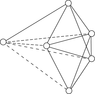
Figure 2. Coxeter diagram for Example 5.3

Appendix A Poles

This appendix is aimed at a discussion of the notion of a pole in a general framework.

A.1. Poles

Let $H$ be a subset of a metric space $X$. A pole of $X$ relative to $H$ (or of the pair $(G,H)$) is a chain of the form $U_{1}\supset U_{2}\supset\dots$, where $U_{k}$ is a non-empty connected component of $X\setminus\mathcal{N}^{X}_{k}(H)$.

A different but equivalent definition of a pole is as follows. Let $\mathscr{H}$ denote the collection of subsets of $X$ at bounded Hausdorff distance from $H$ and let $\mathscr{P}(X)$ be the set of all subsets of $X$. A pole of $X$ relative to $H$ (or of the pair $(X,H)$) is a function $U\colon\mathscr{H}\rightarrow\mathscr{P}(X)$ satisfying the following two conditions, where $H_{1},H_{2}\in\mathscr{H}$:

• $U(H_{1})$ is a non-empty connected component of $X\setminus H_{1}$.

• If $H_{1}\subset H_{2}$, then $U(H_{1})\supset U(H_{2})$.

This equivalent definition makes the following remark obvious.

Remark A.1.

Let $H_{1},H_{2}\subset X$ be at finite Hausdorff distance. Then we can identify the poles of $(X,H_{1})$ with the poles of $(X,H_{2})$.

We now prove that poles are quasi-isometry invariants.

Lemma A.2.

Let $X$ and $Y$ be two path-metric spaces and let $f\colon X\rightarrow Y$ be a quasi-isometry. Then there is a natural correspondence between the poles of $(X,H)$ and the poles of $(Y,f(H))$.

In order to prove Lemma A.2 we will establish the following.

Sublemma A.3.

Let $f\colon X\rightarrow Y$ be a quasi-isometry between a metric space $X$ and a path-metric space $Y$. Then for each $k\in\mathbf{N}$ there is $K\in\mathbf{N}$ such that for each connected component $\alpha$ of $X\setminus\mathcal{N}^{X}_{K}(H)$, there is a connected component $\alpha^{\prime}$ of $Y\setminus\mathcal{N}^{Y}_{k}(f(H))$ satisfying

$$f\big{(}\alpha\big{)}\subset\alpha^{\prime}.$$

Before we provide the proof of Sublemma A.3, we show how to use it in the proof of the lemma.

Proof of Lemma A.2.

Let $V_{1}\supset V_{2}\supset\dots$ be a pole of the pair $(X,H)$. We define its corresponding pole $U_{1}\supset U_{2}\supset\dots$ of $(Y,f(H))$. By Sublemma A.3, for each $k\in\mathbf{N}$ there is a component $U_{k}$ of $Y\setminus\mathcal{N}^{Y}_{k}(f(H))$ which contains the $f$-image of some $V_{K(k)}$. Since all $V_{K(k)}$ intersect, for $k^{\prime}>k$ we have $U_{k}\supset U_{k^{\prime}}$. Thus $U_{1}\supset U_{2}\supset\dots$ is a pole. Hence we have a mapping $f^{\prime}$ from the collection of poles of $(X,H)$ to the collection of poles of $(Y,f(H))$. We now prove that $f^{\prime}$ is a bijection.

Let $g\colon Y\rightarrow X$ be a quasi-isometry which is quasi-inverse to $f$. Let $g^{\prime}$ be the map induced by $g$ which maps the collection of poles of $(Y,f(H))$ to the collection of poles of $(X,g\circ f(H))$. The sets $H$ and $g\circ f(H)$ are at finite Hausdorff distance and by Remark A.1 we can identify the poles of $(X,g\circ f(H))$ with the poles of $(X,H)$. We leave it to the reader to verify that $f^{\prime}\circ g^{\prime}$ and $g^{\prime}\circ f^{\prime}$ are the identity maps. Thus $f^{\prime}$ is a bijection. ∎

It remains to prove the sublemma.

Proof of Sublemma A.3.

We need the following terminology. Given $k\in\mathbf{N}$, a sequence $(x_{0},\dots,x_{n})$ of points in $X$ is called a $k$-path if the distance between any two consecutive $x_{i}$‘s is at most $k$. A subset $Z\subset X$ is called $k$-connected if any two elements of $Z$ may be joined by some $k$-path entirely contained in $Z$.

Let $c$ and $L$ be the additive and the multiplicative constants of the quasi-isometry $f$. Put $K=L(k+L+2c)$. Then $f(X\setminus\mathcal{N}^{X}_{K}(H))$ is contained in $Y\setminus\mathcal{N}^{Y}_{k+L+c}(f(H))$.

Let $\alpha$ be a connected component of $X\setminus\mathcal{N}^{X}_{K}(H)$. The quasi-isometry $f$ maps $\alpha$, which is $1$-connected, to an $(L+c)$-connected subset of $Y\setminus\mathcal{N}^{Y}_{k+L+c}(f(H))$. Any pair of points at distance $L+c$ in $Y\setminus\mathcal{N}^{Y}_{k+L+c}(f(H))$ is connected by a path in $Y$ of length at most $2(L+c)$ (here we use the hypothesis that $Y$ is a path-metric space). This path has to lie in $Y\setminus\mathcal{N}^{Y}_{k}(f(H))$. Hence the points of any connected component $\alpha$ of $X\setminus\mathcal{N}^{X}_{K}(H)$ are mapped into a single connected component of $Y\setminus\mathcal{N}^{Y}_{k}(f(H))$. ∎

We conclude with the following alternative characterisation of poles. A subset of $X$ is called $H$-essential if it is not contained in any tubular neighbourhood of $H$.

Lemma A.4.

1. Suppose that the number of poles of $(X,H)$ is finite and equals $n$. Then for $k$ sufficiently large the number of connected $H$-essential components of the space $X\setminus\mathcal{N}^{X}_{k}(H)$ is exactly $n$.

2. On the other hand, if the number of poles of $(X,H)$ is infinite, then for $k$ sufficiently large the number of connected $H$-essential components of the space $X\setminus\mathcal{N}^{X}_{k}(H)$ is arbitrarily large.

We leave the proof as an exercise to the reader.

A.2. Poles as topological ends

It is natural to ask if the poles of $(X,H)$ may be identified with the topological ends of a certain space. Below we construct such a topological space $X_{\widehat{H}}$ which, as a set, coincides with the disjoint union of $X$ together with one additional point, denoted by $\infty$. The topology on $X_{\widehat{H}}$ is defined in the following way. First, we declare that the embedding $X\to X_{\widehat{H}}$ is continuous and open. Second, we define neighbourhoods of $\infty$ to be complements of those subsets of $X$ which intersect every tubular neighbourhood of $H$ in a bounded subset. In particular, if $H$ is bounded, then $\infty$ is an isolated point.

If $X$ is locally compact, there is an alternative approach. For each $k\in\mathbf{N}$ there is a natural continuous embedding

$$\widehat{\mathcal{N}^{X}_{k}(H)}\to X_{\widehat{H}},$$

where we denote by $\widehat{Z}$ the one-point compactification of a space $Z$. In view of this, the space $X_{\widehat{H}}$ can be alternatively defined as the direct limit of the injective system given by the natural continuous embeddings $\big{\{}\widehat{\mathcal{N}^{X}_{k}(H)}\to\widehat{\mathcal{N}^{X}_{k^{\prime}}(H)}\big{\}}_{k<k^{\prime}}.$

Lemma A.5.

For any compact subset $Q\subset X_{\widehat{H}}$, the intersection $X\cap Q$ is contained in some tubular neighbourhood of $H$.

Proof.

Let $Q\subset X_{\widehat{H}}$ be a subset which contains a sequence $(x_{k})$ of $X$ such that $x_{k}$ does not belong to $\mathcal{N}^{X}_{k}(H)$. Clearly $(x_{k})$ is unbounded in $X$. Moreover, the complement of the set $\{x_{k}\}_{k}$ is a neighbourhood of $\infty$, so that $(x_{k})$ does not sub-converge to $\infty$ in $X_{\widehat{H}}$. This implies that $Q$ is not compact. ∎

Lemma A.5 implies that a sequence $(x_{k})$ in $X$ converges to $\infty$ if and only if it leaves every bounded subset of $X$ but remains in some tubular neighbourhood of $H$. The lemma also immediately implies the following.

Proposition A.6.

There is a natural correspondence between the poles of $(X,H)$ and the topological ends of $X_{\widehat{H}}$.

A.3. Poles in groups

Let now $G$ be a finitely generated group and let $X$ denote the Cayley graph associated with some finite generating set for $G$. We view $X$ as a path-metric space with edges of length $1$. We identify $G$ with the $0$-skeleton $X^{(0)}$ of $X$. Let $H$ be a subset of $G$.

We recall that if $H$ is a subgroup, then $e(G,H)$ denotes the number of relative ends of $G$ with respect to $H$, which are the topological ends of the quotient space $H\backslash X$. This invariant was first introduced by Houghton [Houghton] and Scott [Scott] and is independent of the choice of a generating set for $G$.

On the other hand, we define a pole (in $X$) of $G$ relative to $H$ (or of the pair $(G,H)$) to be a pole of $(X,H)$. By Lemma A.2, there is a correspondence between the collections of poles of the pair $(G,H)$ determined by different generating sets. Hence we can speak about the number of poles of $(G,H)$, which we denote by $\tilde{e}(G,H)$. Here $H$ is allowed to be any subset of $G$.

By Proposition A.6, we have a correspondence between the poles of $(X,H)$ and the ends of the space $X_{\widehat{H}}$. In particular, by Lemma A.2, there is natural correspondence between the ends of $X_{\widehat{H}}$ and the ends of $Y_{\widehat{H}}$, where $Y$ is the Cayley graph of $G$ with respect to a different generating set.

Our notation $\tilde{e}(G,H)$ for the number of poles coincides with the notation of Kropholler and Roller [KR]. Their definition goes as follows.

Let $\mathscr{P}G$ denote the set of all subsets of $G$ and $\mathscr{F}_{H}G$ the collection of all subsets of $G$ contained in $HF$ for some finite subset $F$ of $G$. Notice that an element of $\mathscr{F}_{H}G$ is nothing but a subset of $G$ lying in some tubular neighbourhood of $H$ in the Cayley graph. We view $\mathscr{P}G$ and $\mathscr{F}_{H}G$ as vector spaces over the field $\mathbf{F}_{2}$ of order two.

The action of $G$ on itself by right multiplication preserves both $\mathscr{P}G$ and $\mathscr{F}_{H}G$; they can thus be viewed as right $G$-modules over $\mathbf{F}_{2}$. Kropholler and Roller set

(2) $$\tilde{e}(G,H)=\dim_{\mathbf{F}_{2}}(\mathscr{P}G/\mathscr{F}_{H}G)^{G}.$$

See also Geoghegan [G, Section IV.14] for a similar definition of this value, which is called there the number of filtered ends. We end the appendix by establishing the following.

Lemma A.7.

The number of poles of $(G,H)$ coincides with the value $\tilde{e}(G,H)$ defined by the formula (2).

Proof.

If the number of poles of $(G,H)$ is at least $n$, then there is $k\in\mathbf{N}$ such that $X\setminus\mathcal{N}_{k}^{X}(H)$ has at least $n$ connected $H$-essential components (see Lemma A.4). The set of vertices of each such component determines a non-trivial vector of $(\mathscr{P}G/\mathscr{F}_{H}G)^{G}$. Moreover, the collection of all these vectors is linearly independent. This implies $\tilde{e}(G,H)\geq n$.

Conversely, let $v_{1},\ldots,v_{n}$ be linearly independent vectors in $(\mathscr{P}G/\mathscr{F}_{H}G)^{G}$. Let $V_{i}$ be the subset of $X^{(0)}$ determined by $v_{i}$. Denote by $\partial V_{i}$ the set of all the vertices outside $V_{i}$ which are adjacent to some vertex in $V_{i}$. Then all $\partial V_{i}$ are at finite Hausdorff distance from $H$. Choose $k\in\mathbf{N}$ so that $\mathcal{N}_{k}^{X}(H)$ contains all $\partial V_{i}$. Then each $v_{i}$ lies in the linear subspace of $(\mathscr{P}G/\mathscr{F}_{H}G)^{G}$ determined by the connected $H$-essential components of $X\setminus\mathcal{N}_{k}^{X}(H)$. Hence $n$ is bounded by the number of connected $H$-essential components of $X\setminus\mathcal{N}_{k}^{X}(H)$, which equals at most $\tilde{e}(G,H)$. ∎