Global isomorphism between the Lenard-Jones fluids and the Ising model

Abstract

The interpretation of the linear character of the observable classic rectilinear diameter law and the linear character of the Zeno-line (unit compressibility line $Z=1$) on the basis of global isomorphism between Ising model (Lattice Gas) and simple fluid is proposed. The correct definition of the limiting nontrivial Zeno state is given and its relation with the locus of the critical point is derived within this approach. We show that the liquid-vapor part of the phase diagram of the molecular fluids can be described as the isomorphic image of the phase diagram of the Lattice Gas. It is shown how the the position of the critical points of the fluids of the Lenard-Jones type can be determined basing on the scaling symmetry. As a sequence the explanation of the well known fact about “global“ cubic character of the coexistence curve of the molecular fluids is proposed.

I Introduction

Since the seminal doctoral thesis of van der Waals van der Waals (1873) where the Principle of the Corresponding States was formulated the search for the unifying principles for the description of the variety of thermodynamical properties of complex matter is the key point of statistical physics. By the rigorous methods of the Statistical Mechanics the universal character of the van der Waals (vdW) equation was demonstrated and the numerous extension were proposed Hansen and Mcdonald (2006). The consequences derived from the vdW equation and the observed deviations became the driving force for the further theoretical developments. One of the main achievement of van der Waals was the description of the phase liquid-gas equilibrium which terminated at the corresponding critical point (CP). It opened the possibility to connect the observable thermodynamic quantities with the characteristics of intermolecular interactions. In the modern theory of the Critical Phenomena the ideology of the isomorphism classes of the critical behavior provides the description of the real systems using the results obtained for the model systems like lattice models Baxter (2007). In particular the molecular liquids with short range interactions of the Lenard-Jones (LJ) type belong to the isomorphism class of the Ising model. The latter can be easily mapped to the Lattice Gas (LG) model, which is determined by the Hamiltonian:

$$H=-J\sum\limits_{\left\langle\,ij\,\right\rangle}\,n_{i}\,n_{j}-\mu\,\sum\limits_{i}\,n_{i}\,,$$ (1)

where $n_{i}=0,1$ whether the site is empty or occupied correspondingly. The quantity $J$ is the energy of the site-site interaction of the nearest sites $i$ and $j$, $\mu$ is the chemical potential. The temperature variable corresponding to the Hamiltonian (1) is denoted as $t$. The order parameter is the probability of occupation of the lattice site $x=\left\langle\,n_{i}\,\right\rangle$ and serves as the analog of the density. The phase diagram of the LG is symmetrical with respect to the line $x_{0}=1/2$ and formally extends up to the low temperature region $t\to 0$, where the limiting states $x=0$ and $x=1$ exist only.

Two of the consequences of the vdW equation are of primary importance for our consideration. The first one is the well-known rectilinear law for the diameter of the coexistence curve in terms of the particle density $n$ and the thermodynamic temperature $T$:

$$n_{d}=\frac{n_{liq}+n_{gas}}{2\,n_{c}}=1+A\,\left|\tau\right|+\ldots\,,\quad\tau=\frac{T-T_{c}}{T_{c}}$$ (2)

where $n_{i},\,i=liq,\,gas$ are the values in the corresponding phases, $n_{c},T_{c}$ are the critical density and the temperature. The second fact is another linear law which was derived by Batchinsky Batschinski (1906) long ago from the classical vdW equation:

$$P=\frac{n\,T}{1-n\,b}-a\,n^{2}\,.$$ (3)

The curve defined by the equation $Z=P/(n\,T)=1$ for the compressibility factor $Z$ as it directly follows from Eq. (3) is a straight line:

$$\frac{n}{1/b}+\frac{T}{T^{\text{(vdW)}}_{B}}=1\,.$$ (4)

where $T^{\text{(vdW)}}_{B}=a/b$ is the Boyle temperature determined by the vdW constants in accordance with the virial expansion for Eq. (3). In work of Ben-Amotz and Herschbach Ben-Amotz and Herschbach (1990) the line $Z=1$ is called by the Zeno-line.

Both relations (2) and (5) are approximate and have phenomenological character. But surprisingly they are observed for a wide variety of fluids. As was noted in Guggenheim (1945) the law (2) is fulfilled in rather broad temperature interval of the vapor-liquid phase coexistence region $0.65\lesssim T/T_{c}\lesssim 1$. In the vicinity of the CP the deviations from the linearity become noticeable Mermin (1971); Rehr and Mermin (1973).

In series of works Apfelbaum et al. (2008, 2004, 2006); Apfelbaum and Vorob’ev (2009a, b) the performed analysis of the data for both the real fluids and the systems with model potentials discovered a number of interesting relations between coordinates of the CP, the law of the rectilinear diameter (2) and the Zeno-line:

$$\frac{n}{n_{b}}+\frac{T}{T_{B}}=1\,.$$ (5)

Here $T_{B}$ is the Boyle temperature and for $n_{b}$ the following equation followed from the virial expansion was proposed in Apfelbaum and Vorob’ev (2008):

$$T_{B}=n_{b}\,\frac{B_{3}(T_{B})}{B^{\prime}_{2}(T_{B})}\,.$$ (6)

The phenomenological concept of the “Triangle of Liquid-Gas States“ has been formulated in Apfelbaum et al. (2006). It is heavily based on the cute observation that the Zeno-line is the tangent to the binodal extrapolated to low temperature region. Then the liquid-vapor binodal is inscribed into triangle formed by the straight lines: the coordinate axes $n$ and $T$ and the Zeno-line.

Obviously, the thermodynamic states which satisfy the equation $Z=1$ include the trivial states with negligible density $n\to 0$. This is nothing but the coordinate axis on the thermodynamic $n-T$ plane. Thus the set of the Zeno states is formed by the union of two lines $n=0$ and (5). The statement (5) about the linear nature of Zeno-states is far from trivial. Indeed the expression for $Z$, which for the system with binary potential interaction $\Phi(r_{12})$ reads as (see e.g. Hansen and Mcdonald (2006)):

$$Z=\frac{P}{n\,T}=1-\frac{2\pi\,n}{3\,T}\int r^{3}\frac{\partial\,\Phi(r)}{\partial\,r}\,g_{2}(r;n,T)\,d\,r\,,$$ (7)

where $g_{2}$ is the pair correlation function. Therefore the linearity of the Zeno states is due to quite specific structure of the dependence of correlation function $g_{2}(r;T,n)$ on the thermodynamic state.

Below, following the arguments of previous work Kulinskii (2010), we show that these facts can be casted into elegant geometrical formulation and expand them into general case of the short range power-like attractive potentials in $d$ dimensions. We show that the locus of the CP can be estimated using the correspondence between the scaling properties of the Hamiltonians for the lattice gas and the fluids with the power-like interactive potentials.

II The Zeno-line and the global isomorphism

As was shown in Kulinskii (2010) the linearities of (2) and (5) can be derived on the basis of the assumption of the existence of the global isomorphism of the real liquid-gas part of the phase diagram of the lattice gas model. Note that the line $x=1$ of the LG can be thought of as the analog of the Zeno-line. Indeed the pair correlation function $g_{2}(r)$ of the LG vanishes identically for such “holeless“ states according to the definition. The same is true for the state with empty sites $x=0$. Thus the line $x=0$ can be identified with the zeroth density axes $n=0$ of the real fluid, while the line $x=1$, obviously, can be identified with the Zeno-line $Z=1$. To conserve the linearity and the adjacency properties of the characteristic elements the isomorphism between LG and the fluid should be chosen in the class of the projective mappings Hartshorne (1968) and has the form:

$$n=\,n_{b}\,\frac{x}{1+z\,t}\,,\quad T=\,T_{Z}\,\frac{z\,t}{1+z\,t}\,,$$ (8)

where

$$z=\frac{T_{c}}{T_{Z}-T_{c}}\,.$$ (9)

The coordinates of the CP for the liquid are:

$$n_{c}=\frac{n_{b}}{2\left(\,1+z\,\right)}\,,\quad T_{c}=T_{Z}\,\frac{z}{1+z}\,,$$ (10)

provided that the LG temperature variable $t$ is scaled so that $t_{c}=1$. In view of Eq. (9) it should be noted that if $T_{Z}$ and $n_{b}$ are fixed then the parameter $z$ parameterizes the locus of the CP:

$$\frac{n_{c}}{n_{b}}+\frac{T_{c}}{T_{Z}}=\frac{z+1/2}{1+z}$$ (11)

This means that for the substances belonging to the same class of the corresponding states the loci of the critical points scaled to the $T_{Z}$ and $n_{b}$ lie along the straight line. This correlates with the empirical analysis in Apfelbaum and Vorob’ev (2008). Because both $T_{Z}$ and $T_{c}$ are determined by the interparticle potential the parameter $z$ can be connected with its symmetry properties. Note that all results obtained rely solely on the geometrical facts about phase diagrams of the Lattice Gas and the fluid and do not depend on the specific details of the interactions.

Two limiting Zeno states $T\to 0,\,n\to n_{b}$ and $T\to T_{Z},\,n\to 0$ form the triangle of the Zeno states Apfelbaum et al. (2006). It should be noted that the temperature $T_{Z}$ of the limiting Zeno state with $n_{Z}\to 0$ does not necessary coincide with the Boyle temperature $T_{B}$ as was originally proposed in Apfelbaum et al. (2008). In Apfelbaum et al. (2008) the Boyle state $n\to 0\,,T=T_{B}$ as an obvious limiting Zeno state is used and then the parameter $n_{b}$ is defined by Eq. (6). But any state on $n$-axes can be used in such way. Two limiting Zeno states $n\to 0\,,T=T_{Z}$ and $n=n_{b}\,,T\to 0$ belong to two physically different thermodynamic regions. Therefore there is no apriori physical reasons to define the value $n_{b}$ basing on $T_{B}$. From the point of view of the virial expansion:

$$Z=\frac{P}{n\,T}=1+\sum\limits_{k=1}^{\infty}\,B_{k+1}(T)\,n^{k}$$ (12)

where $B_{k}(T)$ is the virial coefficients Balescu (1975), the limiting state $T_{Z}$ with $n_{Z}\to 0$ is the point where the nontrivial branch of the solution of $Z=1$ emerges from the axis $n=0$ with the specific tangent determined by $T_{Z}$ itself. Clearly the Boyle temperature $T_{B}$ determined by the condition:

$$B_{2}(T_{B})=0\,,$$ (13)

is the simplest choice but in general $T_{Z}\neq T_{B}$ because (13) does not guarantee the correct slope of the Zeno line. Indeed if one search the solution of the equation:

$$Z-1=n\,B_{2}(T)+B_{3}(T)\,n^{2}+\ldots=0$$ (14)

in a form of

$$\frac{n_{Z}}{n_{b}}=1-\frac{T}{T_{Z}}$$ (15)

in the vicinity of $T=T_{Z}$ then obviously the infinitesimal condition:

$$\frac{dZ(n_{Z}(T),T)}{dT}=\left.\frac{\partial\,Z}{\partial\,n}\right|_{T\to T_{Z},\,n\to 0}\,\frac{dn_{Z}}{dT}+\left.\frac{\partial\,Z}{\partial\,T}\right|_{T\to T_{Z},\,n\to 0}=B^{\prime}_{2}(T)+B_{3}\,\frac{dn}{dT}=0$$ (16)

should be fulfilled. Using Eq. (12) we get that $T_{Z}$ is the root of the equation:

$$T_{Z}=n_{b}\,\frac{B_{3}(T_{Z})}{B^{\prime}_{2}(T_{Z})}\,.$$ (17)

This is the rigorous definition of the limiting Zeno state at $n\to 0$ from which the Zeno line emerges. Note that for vdW equation with $B_{2}=b-\frac{a}{T}$, $B_{3}=b^{2}$ and $n_{b}=1/b$, Eq. (17) gives the standard result $T_{Z}=a/b$. Therefore this is the specific property of the vdW equation that the temperatures $T_{Z}$ and $T_{B}$ coincide. Actually the value $T_{Z}$ depends on the dimensionless packing parameter $\eta_{b}=n_{b}\,\sigma^{d}$ in $d$ dimensions, where $\sigma$ is the characteristic scale of the potential, e.g. the hard core diameter. This parameter is determined for the opposite limiting Zeno state with $T\to 0$. Though Eq. (17) formally coincide with Eq. (6), the approach proposed for the determination of the limiting Zeno-state at $n\to 0$ is different from that used in Apfelbaum et al. (2008). Thus the situation is inverse: rather the value $n_{b}$ determines the value $T_{Z}$ and not vice versa. In order to make this consistently with the definition of the Zeno-line we choose $n_{b}$ so that $T_{Z}=T^{\text{(vdW)}}_{B}$, where $T^{(vdW)}_{B}=a/b$ is the Boyle temperature in the van der Waals approximation. We use this to calculate the locus of the critical point in Section IV. Using the standard expressions for the virial coefficients $B_{k}$ for Lenard-Jones potential

$$\Phi(r)=-4U_{0}\left(\,\left(\,\frac{\sigma}{r}\,\right)^{6}-\left(\,\frac{\sigma}{r}\,\right)^{12}\,\right)\,.$$ (18)

the solution of (17) for 3-dimensional system gives $n_{b}\,\sigma^{3}\approx 0.965$ and $T_{Z}=4$ while $T_{B}\approx 3.42$.

III Scale invariant mean-field theory

In this section using the proposed isomorphism we propose the variant of the mean-field approach to calculate the locus of the critical point. It exploits explicitly the scale symmetry which inherent to the power-like interaction potentials. We call it scale-invariant mean-field theory.

Let us show that the parameter $z$ can be determined if the attractive part of the interaction potential possesses the scaling symmetry. The starting point is that using (10) it is easy to derive the following relation:

$$-\frac{d\,\ln{\left(\,T_{c}/T_{Z}\,\right)}}{d\,\ln{\left(\,n_{c}/n_{b}\,\right)}}=\frac{1}{z}$$ (19)

The locus of the CP is determined mostly by the attractive part of the interaction potential and the size of the particles (see e.g. Balescu (1975)). These parameters can be connected with the corresponding ones for the LG model. Suppose that the potential of the $d$-dimensional system is $\Phi(r)=\Phi_{\text{rep}}(r)+\Phi_{\text{attr}}(r)$, where $\Phi_{\text{rep}},\Phi_{\text{attr}}$ are the repulsive and the attractive part correspondingly. Additionally we assume that the attractive part has the power-like behavior $\Phi_{\text{rep}}(r)\sim r^{-(d+\varepsilon)}\,,\varepsilon>0$. Then the corresponding energy of the interaction for the configuration of the number density $n(\mathbf{r})$:

$$E_{\text{int}}=\frac{V}{2}\,\int\Phi(r_{12})\,n(\mathbf{r}_{1})\,n(\mathbf{r}_{2})\,d\mathbf{r}_{12}$$ (20)

can be compared with the LG Hamiltonian (1). Now we put the constraint of the scale invariance of the partition function:

$$\mathcal{Z}=\int\,e^{-E_{\text{int}}/T}\,d\Gamma\,,\quad d\Gamma=\prod\limits_{i=1}^{N}\,d\mathbf{r}_{i}\,,$$ (21)

corresponding to (20) with respect to scaling transformations of $n\to\lambda^{\Delta_{n}}\,n$ and $T\to\lambda^{\Delta_{T}}\,T$, where $\lambda$ is the scale parameter. The exponents $\Delta_{n}$ and $\Delta_{T}$ can be found using standard similarity considerations widely used in condensed matter theory (see e.g. Smirnov (2001)). E.g. for the coordinates of the CP we have:

$$n_{c}\sim\frac{1}{r^{d}_{c}}\,,\quad T_{c}\sim\Phi_{\text{attr}}(r_{c})=\Phi_{\text{attr}}\left(n^{-1/d}_{c}\right)\,,$$ (22)

where $r_{c}$ is the mean interparticle distance in the critical state. Therefore from (19) and (22) we can write the relation:

$$\frac{d\,\ln\left(\,T_{c}/T_{Z}\,\right)}{d\,\ln n_{c}/n_{b}}=\frac{d\,\ln\Phi_{\text{attr}}(n^{-1/d}_{c})}{d\,\ln n_{c}/n_{b}}$$ (23)

which gives the following consistency relation:

$$1/z=1+\varepsilon/d\,.$$ (24)

Thus we obtain the one-parameter group of scaling transformations for the locus of the CP connected with the change of the characteristic scale of the interaction:

$$n_{c}(z)\to\,n_{c}(0)\,\lambda^{-1}\,,\quad T_{c}(z)\to T_{c}(0)\,\lambda^{\left(\,1+\varepsilon/d\,\right)}\,.$$ (25)

Eq. (25) is equivalent to the constraint:

$$n_{c}(\lambda)^{1+\varepsilon/d}\,T_{c}(\lambda)=const\,.$$ (26)

Let us show that Eq. (24) can be considered as some consistency condition between the scaling of for the LG Hamiltonian (1) and that for (20). Note that Eq. (25) represents in particular the scaling of the molecular size $n_{b}$ and corresponding scaling of energy scale given by $T_{B}$ or equivalently $T_{Z}$. To connect the LG model with the LJ fluid where the interaction has the form (20) we take into account that under the scale transformation the loci of the corresponding critical points of these systems should be scaled consistently. Indeed, according to the structure of the LG Hamiltonian (1) the analog of Eq. (26) for the critical point of the LG is as following:

$$x^{2}_{c}\,t_{c}=const\Leftrightarrow\frac{d\,t_{c}}{d\,x_{c}}=-2\,\frac{t_{c}}{x_{c}}\,.$$ (27)

Then the consistency condition between the scaling of the critical point coordinates of the LJ fluid (19) and the Lattice Gas (27) is:

$$\frac{T_{c}/T_{Z}}{n_{c}/n_{b}}\,\left(\,1+\frac{\varepsilon}{d}\,\right)=2\,\quad\Rightarrow\quad\frac{1}{z}=1+\frac{\varepsilon}{d}$$ (28)

In accordance with (8) we get:

$$\frac{T_{c}}{T_{Z}}=\,\frac{1}{2+\frac{\varepsilon}{d}}\,,\quad\frac{n_{c}}{n_{b}}=\,\frac{1+\frac{\varepsilon}{d}}{2\left(\,2+\frac{\varepsilon}{d}\,\right)}\,.$$ (29)

The case of the attractive potential of the van der Waals forces in $d$-dimensions corresponds to $\epsilon=d\,,\,z=1/2$ and we get the estimates:

$$T_{c}=T_{Z}/3\,,\quad n_{c}=n_{b}/3\,.$$ (30)

In the following Section we use (29) to calculate the locus of the critical point of the fluid where the interaction potential is of the LJ type (18).

IV The locus of the critical point for the Lenard-Jones fluid

To test the predictions (29) we compare them with the results of the computer simulations for the potential (18) for $2D$, $4D$ and $5D$ dimension geometries available in Singh et al. (1990); Hloucha and Sandler (1999).

In accordance with the results of Section II we determine the packing parameter $\eta_{b}=n_{b}\,\sigma^{d}$ so that:

$$T_{Z}=T^{(vdW)}_{B}=a/b=\frac{4d}{6-d}\,,\quad a=2^{d-1}\,\frac{4d}{6-d}\,,\quad b=2^{d-1}\,,$$ (31)

where the particle volume $v_{d}(\sigma)$ and $U_{0}$ are put to units. The result are placed in Table 1.

The locus of the CP is obtained easily according to (29) and (31) (see Fig. 1,2). The comparison with the results of the simulations is in Table 2. Note that expressions (29) and (31) allow to clarify the fact noted in Hloucha and Sandler (1999) about different characters of the dependencies of $T_{c}$ and $n_{c}$ on the dimensionality $d$. The value $T_{c}$ strongly depends on the dimension because of the dependence of $T_{B}$ while the $d$-dependence of $n_{c}$ is rather weak.

Note that nonmonotonic dependence of the critical density on the number of dimensions $d$ can be interpreted in terms of the proposed isomorphism as follows. The equilibrium interparticle distance for the LJ potential (18) is $r_{0}=\sigma\,2^{1/6}$ and can be considered as the spacing of the cubic lattice for the LG. The effective radius $r_{\text{eff}}$ of excluded volume occupied by the particle from the physical point of view can be defined by the obvious energetic condition:

$$\Phi(2r_{\text{eff}})=T\quad\Rightarrow\quad r_{\text{eff}}(T)\,.$$ (32)

So the packing of spheres of radii $r_{\text{eff}}$ on the corresponding cubic lattice can be found as

$$\eta(T,d)=\frac{2^{d/6}\,\sigma^{d}}{V(d)\,r_{\text{eff}}(T)^{d}}\,,$$ (33)

where $V(d)=2\frac{\pi^{d/2}}{\Gamma(\frac{d}{2})}$   is the volume of the unit ball in $d$ dimensions. Obviously $n_{c}$ depends on $\eta(T,d)$ monotonically. The dependence of $\eta(T,d)$ on the dimension $d$ is shown on Fig. 2 by grey lines and shows the minimum in the interval $d\leq 4$ in dependence on the temperature. Note that at $T=0$, when $r_{\text{eff}}=\sigma$ this minimum reaches exactly at $d=4$.

LJ “6-12“ fluid	2D	3D	4D	5D
$T_{Z}$	2	4	8	20
$n_{b}\,\sigma^{d}$	0.91	0.965	1.342	2.54
$T_{B}$	1.56	3.418	9.01	40.4

Table 1: The results of computation of $T_{Z}$ and $T_{B}$ for LJ potential (18) for different dimensions and the packing factor $n_{b}\,\sigma^{d}$.

LJ “6-12“ fluid	2D	3D	4D	5D
$T_{c}$	0.5	1.333	3.2	9.08
$T^{(num)}_{c}$, Hloucha and Sandler (1999)	0.515	1.312	3.404	8.8 (?)
$n_{c}$	0.353	0.322	0.404	0.693
$n^{(num)}_{c}$, Hloucha and Sandler (1999)	0.355	0.316	0.34	-

Table 2: The comparison of the estimates (29) with the results of numerical simulations Hloucha and Sandler (1999). The value $T^{5D}_{c}\approx 8.8$ of the critical temperature for $5D$ case was obtained in Hloucha and Sandler (1999) by simple extrapolation of the results for lower dimensions.

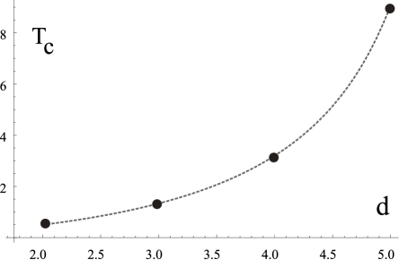
Figure 1: Critical temperature $T_{c}$ for the potential (18) of the $d$-dimensional LJ fluid according to Eq. (29).

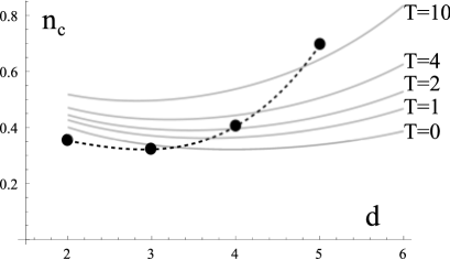
Figure 2: Critical density $n_{c}$ for the potential (18) of the $d$-dimensional according to Eq. (29) (dashed line is the guide for an eye) and the packing fraction $\eta(T,d)$ given by Eq. (33) (grey lines) .

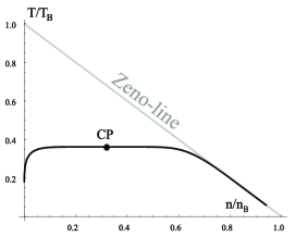
Figure 3: Binodal for 2D Lenard-Jones fluid with $\Phi_{attr}(r)\sim r^{-6}$ calculated as the isomorphic image of the binodal for $2D$ Lattice Gas (Ising model) in accordance with (8).

The existence of global isomorphism also provides the explanation of the fact about the cubic form of the binodal for real molecular fluids. The fact that the shape of the binodal is almost cubic and characterized by the effective exponent $\beta_{eff}=\frac{\partial\,\ln{\varphi}}{\partial\,\ln\tau}\approx 1/3\,,\varphi=\frac{n_{l}-n_{g}}{n_{c}}$ in a wide temperature interval for the system with short range interactions was discovered long ago by J. E. Verschaffelt Verschaffelt (1896); Pitzer (1989); Sengers (1976) (see also Guggenheim (1945)) and since then has been confirmed by the direct numerical simulations Panagiotopoulos (1992); Wilding (1995). In particular in Martynov (2009) the principle possibility to derive the nonclassical exponents for molecular liquids basing on the specific closure of the Ornstein-Zernike equation.

The proposed global isomorphism between LJ fluids and LG leads to the conclusion that the phase coexistence region of the latter is nothing but isomorphic image of the corresponding region of the phase diagram of the LG. For example applying the isomorphism transformation (8) to the known result for 2D Ising model Onsager (1949):

$$x=1/2\pm f(t)^{1/8}\,,\quad f(t)=1-\frac{1}{\sinh^{4}\left(\,2J/t\,\right)}$$ (34)

the binodal for 2D LJ fluid can be easily obtained (see Fig. 3) and compared with the results of the computer simulations Smit and Frenkel (1991). Also the inference that the cubic character of the binodal for real systems is the consequence of the cubic character of the binodal for the Ising model. So one can expect that the coexistence curve of the 3D Ising model is described in the “zeroth approximation“ by the algebraic cubic curve in analogy with (34):

$$x=1/2\pm f(t)^{1/3}\Rightarrow t(x)=f^{-1}\left(\,\left|\,2x-1\,\right|^{3}\,\right)\,,\quad f(1)=0$$ (35)

where $f(t)$ is analytic function of the temperature.

In particular the isomorphism transformation (8) applied to (35) allows to connect the critical amplitude $B_{0}$ for the order parameter of the LJ liquid:

$$\overline{}\frac{n-n_{c}}{n_{c}}=\pm\,B^{\text{(LJ)}}_{0}\,|\tau|^{\beta}+\ldots\,,$$ (36)

with that of the Ising model:

$$2x-1=\pm\,B^{\text{(Is)}}_{0}\,|\,\tau\,|^{\beta}+\ldots\,.$$ (37)

Taking into account the relation (8) between temperature variables $T$ and $t$ via comparison (36) and (37) we obtain the following relation between amplitudes

$$B^{(LJ)}_{0}\approx B^{(Is)}_{0}\,\left(\,1+z\,\right)^{\beta}\,.$$

As the amplitude $B^{(Is)}_{0}$ is known form exact result at $D=2$ or from computer simulation for $D=3$ (see e.g. Talapov and Blote (1996)) one get the critical amplitude for LJ fluid. For the real $3D$ fluids this gives $B_{0}^{(LJ)}\approx 1.69$ for $2D$ case and $B_{0}^{(LJ)}\approx 1.85$ for $3D$ case. Then the proximity of the numerical values of the critical exponents for the systems of the Ising model universality class to the rational numbers is quite natural. They do not necessary close to the mean-field values of the Landau theory and for the systems with the short-range interactions the mean-field behavior is not observed far away from the CP Mon and Binder (1993). This gives the grounds for the universal global cubic law for the binodal proposed in Apfelbaum and Vorob’ev (2008). In essential, the same global cubic law is widely used in computer simulations of the system with short ranged interactions Talapov and Blote (1996); Liu et al. (2006). The fluctuations renormalize these rational exponents near the CP through small exponents $\eta$ and $\alpha$, which determine the behavior of the correlation functions of the density and the entropy in the immediate vicinity of the CP Patashinskii and Pokrovsky (1979). The fluctuations are responsible for the deviation from the linear diameter law (2). If we assume that the transformations between thermodynamic averages like $x$ and $n$ are generated by the transformations between the corresponding microscopic fields then such deviation is interpreted as the consequence of the nonlinearity of the transformation for the field variables. Indeed for the nonlinear functional $F$ of the thermodynamic field $n(\mathbf{r})$ in the presence of strong fluctuations $\left\langle\,F[n(\mathbf{r})]\,\right\rangle\neq F(\left\langle\,n(\mathbf{r})\,\right\rangle)$, where $\left\langle\,\ldots\,\right\rangle$ denotes the statistical average. From this point of view the transformation (8) can be considered as the “mean-field“ analog of commonly used linear mixing of the fields in the vicinity of the CP Rehr and Mermin (1973); Bruce and Wilding (1992).

V Conclusions

In concluding Section we summarize the main results and discuss possible restrictions of the proposed approach.

The whole set of phenomenological facts about the interrelations between Zeno line, the rectilinear diameter, the binodal and the locus of the critical point revealed in Apfelbaum et al. (2004, 2006); Apfelbaum and Vorob’ev (2009a, b) needs in unifying view from the microscopic approach of Statistical Mechanics. The proposed isomorphism allows to search such view in terms of the correspondence between the Hamiltonians of the LG and the fluids with short-ranged pair potentials. In particular it seems natural to connect the thermodynamic potentials for these systems. This allows to determine the parameters of mixing for the fields of the order parameter and the temperature Bruce and Wilding (1992). The results obtained for the locus of the critical point of LJ fluid and critical amplitudes of the equation of state show good correspondence with the results of computer simulations. Though the attractive part of the potential was taken into account in proposed version of the scale invariant mean-field approach the relations Eq. (22),(23) can be generalized to include the repulsive part of the potential. E.g. instead of (23) the following relation arise:

$$\frac{d\,\ln\left(\,T_{c}/T_{Z}\,\right)}{d\,\ln n_{c}/n_{b}}=\frac{d\,\ln\Phi_{\text{attr}}(n^{-1/d}_{c})}{d\,\ln n_{c}/n_{b}}$$

This relation along with the first equation in (10) would give the closed system of equations to determine both $n_{c}$ and $z$ consistently. For the considered case of the LJ potential the repulsive part gives negligible correction so we neglect it here. But in general case the influence of the repulsive part on the locus of the critical point should be taken into account.

Note that the isomorphism relies on simple geometrical facts among which the tangency of the Zeno-line to the extrapolated liquid-vapor binodal into hypothetic region $T\to 0$ is the most crucial Apfelbaum and Vorob’ev (2008). For real systems the liquid branch is restricted by the triple point and this causes the problem of the correct determination of the parameter $n_{b}$. Obviously the slope of the Zeno line at $n_{b}$ influence essentially the position of the opposite Zeno state with $n\to 0$. To overcome this difficulty the correct determination of the limiting Zeno state $(T_{Z},0)$ was proposed along with the determination of $n_{b}$ form the constraint $T_{Z}=a/b$ where $a$ and $b$ are the corresponding van der Waals constants for the equation of states. In principle it is possible to determine the values of $n_{b}$ using the data for the locus of the triple point and the slope of the binodal using the isomorphism transformation which allows to relate this data with the ones for the LG binodal. This will be the subject for further study.

It is interesting to note that in the limit $\varepsilon\to-d$, i.e. when the range of the interaction becomes infinite, $T_{c}\to T_{B}$. Thus the coexistence curve degenerates into triangle. This situation can be compared with the phase diagram for the infinite diluted polymer with the Flory theta-point Flory (1971) (see also in Fisher (1994)).

References

- van der Waals (1873) J. D. van der Waals, Ph.D. thesis, Leiden University, Leiden (1873).
- Hansen and Mcdonald (2006) J.-P. Hansen and I. R. Mcdonald, Theory of Simple Liquids, Third Edition (Academic Press, 2006), ISBN 0123705355.
- Baxter (2007) R. J. Baxter, Exactly Solved Models in Statistical Mechanics (Dover Publications, 2007), ISBN 0486462714.
- Batschinski (1906) A. Batschinski, Ann. Phys. 324, 307 (1906).
- Ben-Amotz and Herschbach (1990) D. Ben-Amotz and D. R. Herschbach, Isr. J. Chem. 30, 59 (1990).
- Guggenheim (1945) E. A. Guggenheim, J. Chem. Phys. 13, 253 (1945), URL http://link.aip.org/link/?JCP/13/253/1.
- Mermin (1971) N. D. Mermin, Phys. Rev. Lett. 26, 169 (1971).
- Rehr and Mermin (1973) J. J. Rehr and N. D. Mermin, Physical Review A 8, 472 (1973), URL http://dx.doi.org/10.1103/PhysRevA.8.472.
- Apfelbaum et al. (2008) E. M. Apfelbaum, V. S. Vorob’ev, and G. A. Martynov, J. Phys. Chem. A 112, 6042 (2008).
- Apfelbaum et al. (2004) E. M. Apfelbaum, V. S. Vorob’ev, and G. A. Martynov, J. Phys. Chem. A 108, 10381 (2004), URL http://dx.doi.org/10.1021/jp046417z.
- Apfelbaum et al. (2006) E. M. Apfelbaum, V. S. Vorob’ev, and G. A. Martynov, J. Phys. Chem. B 110, 8474 (2006).
- Apfelbaum and Vorob’ev (2009a) E. M. Apfelbaum and V. S. Vorob’ev, J. Chem. Phys. 130, 214111 (pages 10) (2009a), URL http://link.aip.org/link/?JCP/130/214111/1.
- Apfelbaum and Vorob’ev (2009b) E. M. Apfelbaum and V. S. Vorob’ev, J. Phys. Chem. B 113, 3521 3526 (2009b).
- Apfelbaum and Vorob’ev (2008) E. M. Apfelbaum and V. S. Vorob’ev, J. Phys. Chem B. 112, 13064 (2008).
- Kulinskii (2010) V. L. Kulinskii, J. Phys. Chem. B 114, 2852 (2010), URL http://pubs.acs.org/doi/full/10.1021/jp911897k.
- Hartshorne (1968) R. Hartshorne, Foundations of Projective Geometry (Addison Wesley Publishing Company, 1968), ISBN 0805337571.
- Balescu (1975) R. Balescu, Equilibrium and Nonequilibrium Statistical Physics (John Wiley & Sons, New York, 1975).
- Smirnov (2001) B. M. Smirnov, Physics-Uspekhi 44, 1229 (2001), URL http://ufn.ru/en/articles/2001/12/b/.
- Singh et al. (1990) R. R. Singh, K. S. Pitzer, J. J. de Pablo, and J. M. Prausnitz, The Journal of Chemical Physics 92, 5463 (1990), URL http://link.aip.org/link/?JCP/92/5463/1.