Dynamic Quantum Tunneling in Mesoscopic Driven Duffing Oscillators

Abstract

We investigate the dynamic quantum tunneling between two attractors of a mesoscopic driven Duffing oscillator. We find that, in addition to inducing remarkable quantum shift of the bifurcation point, the mesoscopic nature also results in a perfect linear scaling behavior for the tunneling rate with the driving distance to the shifted bifurcation point.

I Introduction

In the light of nanomechanics Koz07 and as a qubit readout device for superconducting qubits (i.e., the Josephson bifurcation amplifier) Siddiqi207002 ; Siddiqi027005 ; Devoret014524 ; Mooij119 , the quantum dynamical properties of the driven Duffing oscillator (DDO) gained renewed interest in the past years Katz07 ; Pea06 ; Dyk05 ; Dykman042108 ; Dykman011101 ; MDQT ; low-lying , since these real systems can be well described by a DDO under proper parameter conditions. While some experimental results can be understood by classical means Gro04 ; Gro05 ; Cas07 ; Gro10 , the success of such interpretations is basically due to the fact that the quantum levels are hardly distinguishable from classical nonlinear excitations Gro05 , and the data were classical in origin Gro10 . Actually, possible quantum behaviors and the typical features of the DDO are of great interest to the community mentioned above. For instance, in quasiclassical limit, the quantum feature in the bistable region is investigated against the conventional classical DDO, by simulating a Lindblad-type master equation and comparing the Wigner function with classical probability distribution in phase space Katz07 . Interesting result reached there reveals that the quantum effect makes easier the transition between the bistable states. Moreover, in Refs. Dyk05 ; Dykman042108 ; Dykman011101 ; MDQT , the switching rate between the bistable states near the bifurcation point, owing to quantum and/or thermal fluctuations, were carried out by means of the WKB theory or semiclassical methods such as the mean-first-passage-time approach.

While much more work should be done for unambiguous demonstrations of the quantum behaviors of the DDO, studies of the quantum dynamics of DDO in certain fully quantum regimes are valuable and necessary at the early stage before attacking the whole difficult problem. Indeed, in a fully quantum regime which only involves a few quantum levels of the potential well into the dynamics, quantum behaviors of the DDO such as resonant tunneling and photon-assisted tunneling are discussed in terms of amplitude and phase responses to the driving frequency Pea06 . In the present work, we consider further an intermediate quantum regime, say, the quantum dynamics of a mesoscopic DDO, which involves more than ten quantum levels in the nonlinear dynamics. Obviously, this is a regime between the quantum few-level and the classical dense-level (or continuum) limits note-1 , where the quantum effect should be crucially important, and at the same time the DDO’s nonlinear characteristics can emerge as well. More specifically, we will focus on the dynamic quantum tunneling between the two attractors in the bistable region note-2 , in particular accounting for a quantum shift of the bifurcation point associated with the mesoscopic nature, and extracting a new scaling exponent with the driving distance to the shifted bifurcation point.

II Model and Qualitative Considerations

The DDO is typically described by

$$H_{S}(t)=p^{2}/2m+m\Omega^{2}x^{2}/2-\gamma x^{4}+F(t)x,$$ (1)

where $F(t)=2F_{0}\cos(\nu t)$ stands for the external driving force. Moreover, a DDO is inevitably influenced by its surrounding environment, which can be quantum mechanically modeled by a set of harmonic oscillators, $H_{E}=\sum_{i}(m_{i}\omega_{i}^{2}x_{i}^{2}/2+p_{i}^{2}/2m_{i})$. In a spirit of the Feynman-Vernon-Caldeira-Legget model Wei92 , the coupling between the Duffing oscillator and the environment is well described by $H_{I}=-x\sum_{i}\lambda_{i}x_{i}$. After introducing the spectral density function, $J(\omega)=\pi\sum_{i}\lambda_{i}^{2}\delta(\omega-\omega_{i})/(2m_{i}\omega_{i})$, an important situation is the so-called Ohmic case, corresponding to $J(\omega)=m\kappa\omega\mathrm{exp}(-\omega/\omega_{c})$, where $\kappa$ is the friction coefficient, and $\omega_{c}$ a high frequency cutoff. In the Ohmic case, one can successfully recover the classical friction force Wei92 , which plays an essential role in the classical dynamics of DDO Devoret014524 . In this work, we will employ a master equation approach to simulate the quantum dynamics of DDO. This treatment is equivalent to the (quantum) Langevin equation in which not only the friction but also the fluctuations are taken into account. For the convenience of later use, we also introduce here the operator $b=\sum_{i}\lambda_{i}b_{i}/{\sqrt{2}}$, with $b_{i}=(m_{i}\omega_{i}x_{i}+ip_{i})/{\sqrt{2m_{i}\hbar\omega_{i}}}$.

Notice that the Duffing oscillator described by Eq. (1) has only finite number of bound states. In the absence of external driving, this becomes clear from the so-called soft nonlinearity ($\gamma>0$) potential profile Devoret014524 , $V(x)=\frac{m\Omega^{2}}{2}x^{2}-\gamma x^{4}$, which defines a single well with identical barrier height $V_{0}=m^{2}\Omega^{4}/(16\gamma)$ at $x=\pm\sqrt{m\Omega^{2}/(4\gamma)}$. Nevertheless, compared to the hard nonlinearity ($\gamma<0$) potential well Pea06 , which supports infinite number of bound states, the resultant nonlinear dynamics has no fundamental differences. This is because we are interested in a region not too far from the bottom of the anharmonic potential well. For the soft nonlinearity potential well, the chosen parameters can assure that the unbounded states have negligible effect on the dynamics. This also indicates that the “metastability” to be addressed in the following has no relevance to the “unbounded” states at very high excitations in the soft well. As a rough estimate, the number of bound states is the ratio of $V_{0}$ and $\hbar\Omega$, which gives $N=\frac{m^{2}\Omega^{4}}{16\gamma\hbar\Omega}=\frac{m\Omega}{16\hbar\tilde{\gamma}}=\frac{\aleph}{16\tilde{\gamma}}$. Here we introduced $\aleph\equiv m\Omega/\hbar$, and $\tilde{\gamma}\equiv\gamma/(m\Omega^{2})$. In our model, $\gamma=m\Omega^{2}/24$, so approximately the number of bound state is $3\aleph/2$. In the experiment of Ref. Siddiqi207002 , for instance, a rough estimate gives $\aleph\simeq 366$. In the present work, however, we will set $\aleph\simeq 12$ by altering the circuit parameters. This defines a mesoscopic regime for the DDO with 18 quantum levels involved in the dynamics. Also, we assume an accessible temperature of $5$ mK.

Now we present a qualitative analysis to the driving dynamics of DDO, respectively, in the laboratory frame and in a rotating frame. In Fig. 1(a) we show the energy level diagram of the Duffing oscillator in the absence of driving. To the second-order perturbation of the quartic potential, the energy level reads $E_{n}=[n+1/2-3\tilde{\gamma}(2n^{2}+2n+1)/(4\aleph)]\hbar\Omega$. Accordingly, the adjacent level spacing, $\Delta E_{n}=E_{n}-E_{n-1}=(1-3\tilde{\gamma}n/\aleph)\hbar\Omega$, decreases with $n$. This property, together with a negative frequency detuning (e.g. $\delta=1-{\nu}/{\Omega}=0.065$ in later simulation), would result in the bistability behavior. Qualitatively speaking, for weak driving, the oscillator will largely remain in the initial ground state; for stronger driving, however, it will be increasingly excited to high energy states around $n^{*}$, roughly determined by $\hbar\nu=\Delta E_{n^{*}}$, leading to $n^{*}=\aleph\delta/(3\tilde{\gamma})$.

We notice that an alternative (a better) way to understand the quantum dynamics is in a rotating frame with the driving frequency $\nu$, where the driving field becomes time independent. This can be implemented by applying a rotating transformation ${U}(t)=\mathrm{exp}\{-i\nu t{a}^{\dagger}{a}\}$, where $a\ (a^{\dagger})$ is the annihilation (creation) operator of the DDO. Dropping fast rotating terms, i.e., under the rotating wave approximation (RWA), we obtain ${\tilde{H}_{S}}=\delta[p^{2}/(2m)+(1/2)m\Omega^{2}{x}^{2}]-6\gamma/(4m^{2}\Omega^{4})[{p}^{2}/(2m)+(1/2)m\Omega^{2}{x}^{2}]^{2}+F_{0}{x}.$ In the absence of driving, this rotated Hamiltonian is naturally diagonal, with the eigenstates of harmonic oscillator ${\psi}_{n}$, and eigenvalues $\tilde{E}_{n}=[n+1/2-3\tilde{\gamma}/(2\aleph\delta)(n+1/2)^{2}]\hbar\delta\Omega$, as schematically shown in Fig. 1(b). Interestingly, we find here that the $n^{*}$th level is the highest one (noting that $n^{*}$ labels the resonant level-pair in the laboratory frame). Also, the level spacing in the rotating frame is much smaller than its counterpart in the laboratory frame. Then, it is clear that the DDO’s dynamics in this rotating frame is governed by the interplay of $F_{0}x$-induced transition and environmental dissipation. More interestingly, in the presence of $F_{0}x$, we can diagonalize the transformed Hamiltonian $\tilde{H}_{S}$, and denote the eigenstates by $\tilde{\psi}_{n}$. It is found that a one-to-one correspondence exists between $\psi_{n}$ and $\tilde{\psi}_{n}$, which can be understood in the spirit of adiabatic switching. Then, we may regard $\tilde{\psi}_{n^{*}}$- and $\tilde{\psi}_{0}$-dominated states (wavepackets) as two attractors, which direct the evolution, determine the final state, and are responsible to the bistable behavior. Here we may mention that the classical dynamics of DDO can lead to possible chaotic motion, see, for instance, a brief discussion in Ref. Devoret014524 . For the purpose of quantum detector applications, however, the chaotic motion should be avoided by setting a low bound of detuning Devoret014524 . In the present work, as we did previously in Ref. Guo10 , we have similarly set an upper bound of detuning in order to eliminate the possible chaotic motion. In the mesoscopic regime, the $\tilde{\psi}_{n^{*}}$- and $\tilde{\psi}_{0}$-dominated wavepackets, which can be regarded as the counterparts of classical attractors, consist of a couple of discrete states. In the following, these “quantized” attractors will be named also small amplitude state (SAS) and large amplitude state (LAS).

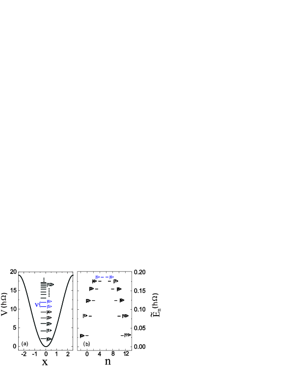
Figure 1: (Color online) Energy diagram of the non-driven Duffing oscillator in (a) the laboratory frame, and (b) the rotating frame.

III Master Equation in Rotating Frame

To account for the environmental effects on the DDO, a Lindblad-type master equation can be employed Katz07 ; Dykman042108 ; Dykman011101 ; low-lying , simply following the typical treatment for cavity photons (oscillators) in quantum optics. In this work, however, viewing the “$x$-$x_{j}$” type interaction assumed by the Feynman-Vernon-Caldeira-Legget model which is actually beyond the rotating wave approximations Katz07 ; Dykman042108 ; Dykman011101 ; low-lying , we would like to use a different type of master equation, say, the Born-Markov-Redfield (BMR) version Tan97 ; Yan98 ; Sch98 , to study the quantum dynamics of a weakly damped DDO as it is. Following the notation proposed in Ref. Yan98 , the BMR master equation for DDO’s reduced density matrix reads

$$\dot{\rho}(t)=-i\hbar^{-1}\mathcal{L}_{S}\rho(t)-\hbar^{-2}\int_{0}^{t}d\tau\langle\mathcal{L}_{I}(t)\mathcal{G}(t,\tau)\mathcal{L}_{I}(\tau)\mathcal{G}^{\dagger}(t,\tau)\rangle\rho(t).$$ (2)

Here $\mathcal{L}_{S}(\cdots)=[H_{S},(\cdots)]$ is associated with the DDO Hamiltonian in laboratory frame, while $\mathcal{G}(t,\tau)(\cdots)=G(t,\tau)(\cdots)G^{\dagger}(t,\tau)$ is the propagator in Liouvillian space. The interaction Liouvillian $\mathcal{L}_{I}$ is defined by $\mathcal{L}_{I}(\cdots)=[{H_{I}},(\cdots)]$, where $H_{I}=-x\sum_{j}\lambda_{j}x_{j}\equiv-xX_{E}$ describes the coupling of DDO to environment. The average in Eq. (2) means $\langle(\cdots)\rangle=\mathrm{tr}_{E}[(\cdots)\rho_{E}]$, with $\rho_{E}$ the thermal equilibrium density operator of the environment. In laboratory frame, the driving in $H_{S}$ is time-dependent, which would complicate the dissipation terms in Eq. (2) and make the numerical simulation difficult. To overcome this difficulty, we transform Eq. (2) into the rotating frame: $\dot{\tilde{\rho}}(t)=-i\hbar^{-1}\tilde{\mathcal{L}}_{S}\tilde{\rho}(t)-\hbar^{-2}\int_{0}^{t}d\tau\langle\tilde{\mathcal{L}}_{I}(t)\tilde{\mathcal{G}}(t,\tau)\tilde{\mathcal{L}}_{I}(\tau)\tilde{\mathcal{G}}^{\dagger}(t,\tau)\rangle\tilde{\rho}(t)$. Here, the various transformed quantities are defined as: $\tilde{\rho}(t)={U}^{\dagger}\rho(t){U}$, $\tilde{\mathcal{L}}_{S}(\cdots)=[{U}^{\dagger}{H_{S}}{U}+i\hbar\dot{{U}}^{\dagger}{U},(\cdots)]=[{\tilde{H}_{S}},(\cdots)]$, $\tilde{\mathcal{L}}_{I}(\cdots)=[{U}^{\dagger}{H_{I}}{U},(\cdots)]=[{\tilde{H}_{I}},(\cdots)]$, and $\tilde{\mathcal{G}}(t,\tau)$ is the propagator associated with ${\tilde{H}_{S}}$. Note that in the rotating frame the coupling Hamiltonian becomes time dependent, i.e., ${\tilde{H}_{I}}=-U^{\dagger}xUX_{E}=-\sqrt{\hbar/2m\Omega}({a}^{\dagger}e^{i\nu t}+{a}e^{-i\nu t})X_{E}$. Inserting this result into the EOM of $\tilde{\rho}(t)$ yields

$$\dot{\tilde{\rho}}(t)=-i\hbar^{-1}\tilde{\mathcal{L}}_{S}\tilde{\rho}(t)-\frac{1}{4\aleph}\{[{a}^{\dagger},(C(-\tilde{\mathcal{L}}_{S}+\nu){a})\tilde{\rho}]$$

$$~{}~{}~{}+[{a},(C(-\tilde{\mathcal{L}}_{S}-\nu){a}^{\dagger})\tilde{\rho}]+e^{i2\nu t}[{a}^{\dagger},(C(-\tilde{\mathcal{L}}_{S}-\nu){a}^{\dagger})\tilde{\rho}]$$

$$~{}~{}~{}+e^{-i2\nu t}[{a},(C(-\tilde{\mathcal{L}}_{S}+\nu){a})\tilde{\rho}]+{\rm H.c.}\}.$$ (3)

In deriving this result, the well established Markov-Redfield approximation has been applied. Accordingly, the spectral function, $C(\tilde{\mathcal{L}}_{S})$, is a Fourier transform of the environment correlator: $C(\tilde{\mathcal{L}}_{S})=\int_{-\infty}^{+\infty}dtC(t)e^{i\hbar^{-1}\tilde{\mathcal{L}}_{S}t}$, and $C(t)=\mathrm{Tr}_{E}[{X_{E}}(t){X_{E}}(0)\rho_{E}]$.

Eq. (III) is the desired equation we obtain in the rotating frame. To relate it with other work, we first drop the fast oscillating terms in Eq. (III) under the rotating wave approximation. Then, we assume further a harmonic approximation: $\tilde{\mathcal{L}}_{S}a\approx-\hbar\delta\Omega a$, and $\tilde{\mathcal{L}}_{S}a^{\dagger}\approx\hbar\delta\Omega a^{\dagger}$. As a result, the well-known Lindblad master equation is obtained: $\dot{\tilde{\rho}}(t)=-i\hbar^{-1}\tilde{\mathcal{L}}_{S}\tilde{\rho}(t)+\kappa\{[1+n(\Omega)]{\cal D}[a]\tilde{\rho}+n(\Omega){\cal D}[a^{\dagger}]\tilde{\rho}\}$ , where the Lindblad superoperator is defined through ${\cal D}[A]\tilde{\rho}\equiv A\tilde{\rho}A^{\dagger}-\frac{1}{2}\{A^{\dagger}A,\tilde{\rho}\}$. In obtaining this result, the explicit form of the spectral function has been used, i.e., $C(\omega)=2[1+n(\omega)]J(\omega)$, where $n(\omega)$ is the Bose function. We notice that in Ref. Dykman011101 the study of quantum activation was actually based on this same equation, together also with a few techniques and approximations involved in the later analysis.

IV Quantum Shift of the Bifurcation Point

For comparative purpose, we first outline the result from a classical analysis. It is well known that the classical DDO obeys Devoret014524 : $m\ddot{{x}}+m\Omega^{2}{x}+m\kappa\dot{{x}}-4\gamma{x}^{3}=-F(t)$. Define dimensionless variables $\tau=\Omega t$, $w=\nu/\Omega$, $f=\sqrt{{4\gamma}/({m^{3}\Omega^{6}}})2F_{0}$, $Q=\Omega/\kappa$, and $\Delta=-2Q\delta$; and introduce rotating transformation $x(\tau)=[\tilde{x}(\tau)e^{iw\tau}/2+c.c.]/\sqrt{{4\gamma}/({m\Omega^{2}}})$. Then the slowly varying amplitude $\tilde{x}(\tau)$ of the DDO in the rotating frame satisfies the following EOM Devoret014524 : $2i\dot{\tilde{x}}(\tau)=[(\Delta-i)/Q+3|\tilde{x}|^{2}/4]\tilde{x}-f$. Stationary solution of this equation yields a bistability diagram as shown in Fig. 2(a). Moreover, two critical driving strengths, $f_{B}(\Delta)$ and $f_{\bar{B}}(\Delta)$, can be obtained in the limit $Q\gg 1$: $f_{B,\bar{B}}(\Delta/\Delta_{c})=f_{c}/(2x^{3/2})\sqrt{1+3x^{2}\pm(1-x^{2})^{3/2}}|_{x=\Delta_{c}/\Delta}$. Here $\Delta_{c}=-\sqrt{3}$, and $f_{c}=2^{5/2}/(3^{5/4}\sqrt{\Delta^{3}})$. Accordingly, after restoring dimensional units, the critical driving strengths read $F_{B,\bar{B}}=\sqrt{m^{3}\Omega^{6}/(16\gamma)}f_{B,\bar{B}}$. In what follows, we will focus on the most important upper point $F_{B}$, which is to be re-denoted as $F_{c}$ and taken as the unit of the driving force.

Unfortunately, in mesoscopic regime, as we will see later, the critical driving strength $F_{c}$ determined above does not match the result from numerical simulation. It would thus be desirable to develop a quantum version for the EOM of $\tilde{x}(\tau)$, in order to reach consensus with the direct numerical simulation. Following Ref. Joo03 , given that the reduced density matrix satisfies the Lindblad master equation, in Heisenberg picture the operator $a$ should obey an equation of motion as follows

$$\dot{a}(t)=-i\hbar^{-1}[a,\tilde{H}_{S}]+\kappa\bar{\cal D}[a]a=-i\hbar^{-1}[a,\tilde{H}_{S}]-\frac{\kappa}{2}a,$$ (4)

where the dual-Lindblad superoperator is defined through $\bar{\cal D}[A]a\equiv A^{\dagger}aA-\frac{1}{2}\{A^{\dagger}A,a\}$. Here we assumed the low temperature limit $n(\Omega)\ll 1$. Moreover, below $F_{c}$ and starting with a small-amplitude state, the subsequent evolution will largely remain in a coherent state Kni05 ; Khe99 ; note-3 . Then, in coherent state representation and relating the coherence number $\alpha(\tau)$ with a complex amplitude $\tilde{x}(\tau)=\sqrt{8\gamma/(m\Omega^{2})}\alpha(\tau)/\sqrt{n}$, from Eq. (4) we obtain the same EOM for $\tilde{x}(\tau)$ as above, but with a quantum mechanically shifted detuning

$$\tilde{\Delta}=-2Q(\delta-3\tilde{\gamma}/\aleph),$$ (5)

instead of the classical result $\Delta=-2Q\delta$. In classical case, $\aleph$ is large, e.g., $\aleph\simeq 366$ as we estimated from the experimental circuit parameters, which makes the quantum shift negligibly small. Nevertheless, in mesoscopic regime, e.g., $\aleph\simeq 12$ in present case, this quantum shift cannot be neglected, as shown in Fig. 2(b) and (c), where the critical driving strength moves to $0.77F_{c}$. Below we illustrate this quantum shift in phase space in terms of the Wigner function.

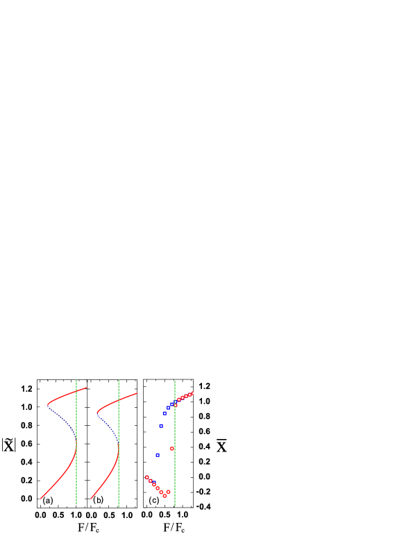
Figure 2: (Color online) (a) and (b): Bifurcation diagram of the DDO based on the EOM of $\tilde{x}(\tau)$, (a) without and (b) with accounting for the quantum shift of the effective detuning [see Eq. (5)]. The dashed vertical lines indicate the respective bifurcation points. (c): Results from numerical simulation of $\bar{x}(t)$ =$\mathrm{Tr}[{x}\tilde{\rho}(t)]$ based on Eq. (III). We choose the $\bar{x}(t)$ at $t=160*(2\pi/\Omega)$ to represent the steady state amplitude $\bar{x}$. The circles and squares stand for results from different initial conditions (i.e. the SAS and LAS), from which we observe the hysteresis behavior. Here, again, the dashed vertical line indicates the bifurcation point in (b), say, $0.77F_{c}$, which agrees well with the numerical simulation. Parameters: $\kappa=0.01$, $T$=5mK, $\delta=0.065$, and $\aleph=12$.

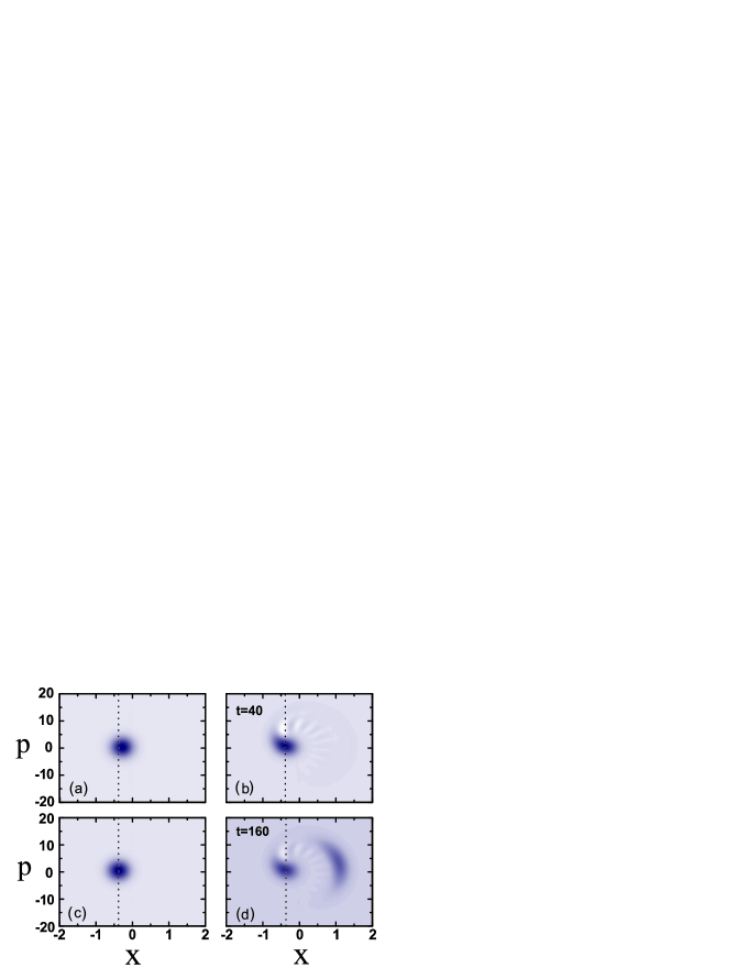
Figure 3: (Color online) (a) and (b): Wigner function of the coherent state determined from the steady-state solution of the EOM of $\tilde{x}(\tau)$, (a) without and (b) with accounting for the quantum shift. (c) and (d): Wigner function from numerical simulation based on Eq. (III), at $t=40*(2\pi/\Omega)$ and $160*(2\pi/\Omega)$, respectively. The dashed vertical line in each sub-figure indicates the valid “$x$” center of Wigner function of the SAS. Parameters: $\kappa=0.01$, $T$=5mK, $\delta=0.065$, $\aleph=12$, and $F_{0}=0.7F_{c}$.

The Wigner function is defined as: $W(x,p,t)=1/(\pi\hbar)\int_{-\infty}^{+\infty}\langle x+x^{\prime}|\rho(t)|x-x^{\prime}\rangle\exp(-i2px^{\prime}/\hbar)dx^{\prime}$. In Fig. 3(a) and (b), for comparative purpose, we plot the Wigner function simply using $\tilde{\rho}_{s}\equiv|\alpha\rangle\langle\alpha|$, where the coherence number $\alpha$ is determined from $\tilde{x}$, based on the steady-state solution of the amplitude EOM without and with accounting for the quantum shift, while in Fig. 3(c) and (d) we show the results from direct simulation. We see that in mesoscopic regime it is essential to account for the quantum shift, in order to make the amplitude EOM agree with numerical simulation, as indicated by the dashed vertical lines in Fig. 3. (The vertical line in each sub-figure indicates the valid “$x$” center of Wigner function of the SAS.) It is then observed that the classical result in Fig. 3(a) has considerable deviation. Moreover, from Fig. 3(d) we get an insight that starting on from certain transient stage, the oscillator evolves into a mixed state, which can be formally expressed as: $W(x,p,t)=P_{S}(t)W_{S}(x,p)+P_{L}(t)W_{L}(x,p,t)$. Here, $W_{S}(x,p)$ and $W_{L}(x,p,t)$ are the Wigner functions of the intrinsic SAS and LAS, say, the two attractors, while $P_{S}(t)$ and $P_{L}(t)$ are the respective occupation probabilities.

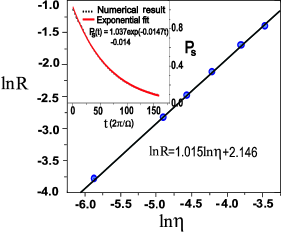
Figure 4: (Color online) Scaling behavior of the dynamic quantum tunneling rate with the driving distance to the shifted bifurcation point, say, $\eta=(0.77F_{c})^{2}-F_{0}^{2}$. Here, the circles are result from numerical simulation, while the linear fit gives $\alpha=1.015$ for the tunneling action $R\varpropto\eta^{\alpha}$. Inset: an illustrative example of exponential fitting for the occupation probability of the SAS, under driving $F_{0}=0.76F_{c}$. Parameters: $\kappa=0.01$, $T$=5mK, $\delta=0.065$, and $\aleph=12$.

V Tunneling Rate and Scaling Exponent

Based on the structure of the mixed state $W(x,p,t)$, we can formulate a way to determine the dynamic tunneling rate from SAS to LAS as follows. Originally, in laboratory frame, this rate can be extracted from the occupation probability of the SAS via $\Gamma_{t}=-dP_{S}(t)/dt$, while $P_{S}(t)=\langle\alpha e^{i\nu t}|\rho(t)|\alpha e^{i\nu t}\rangle$. Note that here we have used the fact that the SAS in laboratory frame is a rotating coherent state. More conveniently, transformed to the rotating frame, $P_{S}(t)=\mathrm{Tr}[\tilde{\rho}_{s}\tilde{\rho}(t)]$, where $\tilde{\rho}_{s}\equiv U^{\dagger}(t)\rho_{s}(t)U(t)=|\alpha\rangle\langle\alpha|$ is static, and $\tilde{\rho}(t)=U^{\dagger}(t)\rho(t)U(t)$ is the DDO state in the rotating frame described by Eq. (III).

In the inset of Fig. 4 we show a representative $P_{S}(t)$, obtained from numerical simulation using Eq. (III) and the formalism outlined above, from which we see that a single exponential fit can well characterize $P_{S}(t)$. This indicates nothing but a rate process from SAS to LAS. Moreover, the success of a single exponential fit indicates a dominant forward process from SAS to LAS. That is, at the early escape stage, the backward process from LAS to SAS has not yet happened. This is similar to the situation in determining the tunneling rate in double-well problem, where the backward tunneling process is negligibly small at certain early time stage.

Therefore, using this numerical approach we can extract the dynamic tunneling rate ($\Gamma_{t}$) from SAS to LAS. Further, following Ref. Dykman011101 , we assume $\Gamma_{t}=Ce^{-R/\lambda}$. In this proposed form, $C$ is an irrelevant prefactor, while the exponential factor $e^{-R/\lambda}$ originates from an effective activation process. In limiting cases, such as for classical thermal activation, $R$ is the activation energy and $\lambda$ the temperature; while for quantum tunneling through a barrier, $R$ is the tunneling action and $\lambda$ the Plank constant. In our present case, it is a generalization. We may view $R$ as an effective activation energy and $\lambda$ an effective Planck constant or temperature.

Very interestingly, it was found in Ref. Dykman011101 that the dynamic tunneling action $R$ displays a perfect scaling behavior with the driving distance to the critical point, which is defined as $\eta=F_{c}^{2}-F^{2}_{0}$. Quantitatively, it was found $R\varpropto\eta^{\alpha}$ and $\alpha=3/2$. Here, for the mesoscopic DDO, owing to the quantum shift of the critical point, which moves to $0.77F_{c}$ under the assumed parameter condition as shown in Fig. 2, we define accordingly the driving distance as $\eta=(0.77F_{c})^{2}-F^{2}_{0}$. Remarkably, we demonstrate in Fig. 4 that the scaling behavior of $R\varpropto\eta^{\alpha}$ still holds, yet with an alternative scaling exponent, $\alpha\simeq 1$, instead of $\alpha=3/2$ as found by Dykman Dykman011101 .

We noticed that in Ref. Sta06 , scaling behavior of the transition rate with the driving frequency (but not the driving strength) was analyzed to give $\alpha\simeq 1.3\sim 1.4$, by a rough fitting from a few experimental data. Meanwhile, in the experiments by Siddiqi et al. Sid0305 , an effective potential with a barrier height scaled as $\Delta U^{0}_{dyn}\propto\left[1-(F_{0}/F_{c})^{2}\right]^{3/2}$, was employed to analyze their measured data. By means of a thermal-activation rate $\propto\exp\left(-\Delta U^{0}_{dyn}/k_{B}T\right)$, this would result in a scaling exponent $\alpha=3/2$, while a rough quantum WKB estimate for the quantum tunneling rate $\propto\exp\left(-\sqrt{\Delta U^{0}_{dyn}}a/\hbar\right)$, where $a$ is an effective width of the barrier, is seemingly to give $\alpha=3/4$.

Moreover, in Ref. Dyk05 , it was shown that both the exponents “3/2” and “1” can be obtained, respectively, resulting from a local and nonlocal Hamiltonian bifurcation. Nevertheless, we should distinguish Ref. Dyk05 from our present study in at least two aspects: (i) The rates obtained in Ref. Dyk05 are classical ones, i.e., the thermal-activation-caused escape rates, since they are respectively related to an “effective potential” that is then inserted into the thermal-activation rate formula. (ii) For the DDO model under our present study, the “local bifurcation” is near the larger bifurcation point, and the “nonlocal bifurcation” is close to the smaller one. This clarification is clearly stated in Sec VII of Ref. Dyk05 . Our numerical study, however, is focused on the region near the larger bifurcation point, thus should correspond to the “local bifurcation”, and should be compared with the exponent “3/2”.

In a recent workGuo10 , we performed a real time simulation for the quantum dynamics of the mesoscopic DDO in laboratory frame, in which the driving field was not taken into account in the dissipation terms. Also, in Ref. Guo10 , the quantum shift was canceled owing to the extra term “$x^{2}\sum_{i}\lambda_{i}^{2}/(2m_{i}\omega_{i}^{2})$” in the Caldeira-Legget model. In the present work, however, absorbing this term into the system Hamiltonian, which effectively renormalizes the DDO’s frequency, makes the quantum shift evident. In regard to the scaling behavior, quite desirably, both studies of Ref. Guo10 and the present one give consistent result. This strongly implies that the scaling exponent $\alpha=3/2$ is non-universal, and $\alpha=1$ is an alternate scaling exponent in the mesoscoic regime. Further investigation for the crossover behavior from a mesoscopic to the usual classical regime is of particular interest. However, such kind of study will encounter increasing difficulty in real time simulation, which is to be the task of our forthcoming research.

VI Summary

To summarize, in a mesoscopic regime we investigated the dynamic quantum tunneling of the driven Duffing oscillator. Owing to the mesoscopic nature, we found that the critical driving strength has a quantum shift, and the tunneling action (extracted exponentially from the tunneling rate) exhibits a perfect linear scaling behavior with the driving distance to the quantum shifted critical point.

Acknowledgements.— This work was supported by the National Natural Science Foundation of China, the 973 project, the Fundamental Research Fund for Central Universities, and the Fund for Doctoral Training.

References

- (1) I. Kozinsky, H. Postma, O. Kogan, A. Husain, and M. Roukes, Phys. Rev. Lett. 99, 207201(2007).
- (2) I. Siddiqi et al., Phys. Rev. Lett. 93, 207002 (2004); I. Siddiqi et al., Phys. Rev. Lett. 94, 027005 (2005).
- (3) I. Siddiqi et al., Phys. Rev. B 73, 054510 (2006).
- (4) V. E. Manucharyan et al., Phys. Rev. B 76, 014524 (2007).
- (5) A. Lupascu et al., Nat. Phys. 3, 119 (2007).
- (6) I. Katz, A. Retzker, R. Straub, and R. Lifshitz, Phys. Rev. Lett. 99, 040404 (2007); I. Katz, R. Lifshitz, A. Retzker, and R. Straub, New J. Phys. 10, 125023 (2008).
- (7) V. Peano and M. Thorwart, Phys. Rev. B 70, 235401 (2004); Chem. Phys. 322, 135 (2006); New J. Phys. 8, 21 (2006).
- (8) M. I. Dykman, I. B. Schwartz, and M. Shapiro, Phys. Rev. E 72, 021102 (2005).
- (9) M. Marthaler and M. I. Dykman, Phys. Rev. A 73, 042108 (2006).
- (10) M. I. Dykman, Phys. Rev. E 75, 011101 (2007).
- (11) I. Serban and F. K. Wilhelm, Phys. Rev. Lett. 99, 137001 (2007).
- (12) M. A. Armen and H. Mabuchi, Phys. Rev. A 73, 063801 (2006).
- (13) N. Gronbech-Jensen et al., Phys. Rev. Lett. 93, 107002 (2004).
- (14) N. Gronbech-Jensen and M. Cirillo, Phys. Rev. Lett. 95, 067001 (2005).
- (15) M. G. Castellano et al., Phys. Rev. Lett. 98, 177002 (2007);
- (16) N. Gronbech-Jensen, J.E. Marchese1, M. Cirillo, and J.A. Blackburn, Phys. Rev. Lett. 105, 010501 (2010).
- (17) Actually, in our numerical simulations, about “18” bound states will be involved in the nonlinear dynamics. We noticed that in Ref. Katz07 about “60” states are involved in the dynamics, corresponding to a quasiclassical limit. While in the papers by Peano and Thorwart Pea06 , where the nonlinear term of the potential is positive, thus can support arbitrary number of bound states, only a few number of states (about “8”) are involved in the dynamics, implying a “deep quantum regime”. The term “mesoscopic” we used in our work basically means that the number of relevant (bound) states in the dynamics is in an intermediate range, i.e., between “a few” and “a large” number of states.
- (18) In this work, following Ref. MDQT , we use the term “dynamic quantum tunneling” to describe the quantum transition between the metastable states in the bistable region. For a driven dynamic system, the phase space can have classically forbidden areas even in the absence of potential barriers. Quantum mechanically, however, these areas can be crossed in a process called dynamical tunneling (see MDQT and references therein). As a matter of fact, this is exactly the same process as studied in Ref. Dykman042108 where the term “quantum activation” is employed, noting that it also describes the escape from a metastable state due to quantum fluctuations that lead to diffusion away from the metastable state and, ultimately, to transition over the classical “barrier”, that is, the boundary of the basin of attraction to the metastable state.
- (19) U. Weiss, Quantum Dissipative Systems (World Scientific, Singapore, 2nd Ed., 1999).
- (20) L.Z. Guo, Z.G. Zheng, and X.Q. Li, Europhys. Lett. 90, 10011 (2010).
- (21) D. Kohen, C. C. Marston, and D. J. Tannor, J. Chem. Phys. 107, 5236 (1997).
- (22) Y.J. Yan, Phys. Rev. A 58, 2721(1998); Y.J. Yan and R.X. Xu, Phys. Rev. E 75, 031107 (2007).
- (23) A. Shnirman and G. Schön, Phys. Rev. B 57, 15 400 (1998); Yu. Makhlin, G. Schön, and A. Shnirman, Rev. Mod. Phys. 73, 357 (2001).
- (24) E. Joos et al., Decoherence and the Appearance of a Classical World in Quantum Theory (Springer-Verlag, 2nd Ed., 2003), p. 332.
- (25) C. Gerry and P. Knight, Introductory Quantum Optics (Cambridge University Press, 2005), p. 208.
- (26) K.V. Kheruntsyan, J. Opt. B: Quantum Semiclass. Opt. 1, 225 (1999).
- (27) That the SAS is an approximate coherent state can be understood as follows. For a dissipative harmonic oscillator described by a Lindblad master equation, e.g., a damping optical cavity under laser driving, the stationary state is exactly a coherent state. An elegant proving for this can be found in the book Kni05 . For the DDO problem, since the SAS is near the bottom of the potential well where the anharmonicity is negligible, we can then expect that the SAS is an approximate coherent state.
- (28) C. Stambaugh and H.B. Chan, Phys. Rev. B 73, 172302 (2006).
- (29) I. Siddiqi, R. Vijay, F. Pierre, C.M. Wilson, M. Metcalfe, C. Rigetti, L. Frunzio, and M.H. Devoret, arXiv:condmat/ 0312623; I. Siddiqi, R. Vijay, F. Pierre, C.M. Wilson, L. Frunzio, M. Metcalfe, C. Rigetti, and M.H. Devoret, arXiv:cond-mat/0507248.