Melting and Rippling Phenomena in Two Dimensional Crystals with localized bonding

Abstract

We calculate Root Mean Square (RMS) deviations from equilibrium for atoms in a two dimensional crystal with local (e.g. covalent) bonding between close neighbors. Large scale Monte Carlo calculations are in good agreement with analytical results obtained in the harmonic approximation. When motion is restricted to the plane, we find a slow (logarithmic) increase in fluctuations of the atoms about their equilibrium positions as the crystals are made larger and larger. We take into account fluctuations perpendicular to the lattice plane, manifest as undulating ripples, by examining dual-layer systems with coupling between the layers to impart local rigidly (i.e. as in sheets of graphene made stiff by their finite thickness). Surprisingly, we find a rapid divergence with increasing system size in the vertical mean square deviations, independent of the strength of the interplanar coupling. We consider an attractive coupling to a flat substrate, finding that even a weak attraction significantly limits the amplitude and average wavelength of the ripples. We verify our results are generic by examining a variety of distinct geometries, obtaining the same phenomena in each case.

I Introduction

Efforts to gain a quantitative microscopic understanding of melting have spanned more than a century. The Lindemann criterion developed in 1910 Lindemann (1910) describes melting in terms of the Root Mean Square (RMS) deviation from the atomic equilibrium positions. Since long-range positional order stems from the periodic arrangement of atoms in crystalline solid, atomic deviations that are comparable to the separation between atomic species could obscure the regularity of the underlying crystal lattice with a concomitant loss of positional order. The Lindemann criterion specifies that melting has occurred if the RMS deviations reach on the order of a tenth of a lattice constant, and has proved to be a reasonably effective theory for three dimensional systems.

The Lindemann analysis does not take into account correlations of the motions of neighboring atoms. Correlations are more important at lower dimensions, and the process of melting is hence strongly dimensionally dependent. While three dimensional crystals exhibit long-range order below certain temperatures, statistical fluctuations play a significant role in one dimensional systems, precluding all but short-ranged local ordering for $T>0$.

The process of melting in two dimensions is more subtle, and is understood in the modern context to occur in more than one stage. An initial continuous loss of positional order precedes the proliferation of lattice defects, which accumulate and eventually complete the melting process at sufficiently high temperatures by destroying even orientational order, where each atom has a fixed number of neighbors.

Thermally induced fluctuations in atomic positions can have an important effect on nano-engineered systems where structures may be on the atomic scale. Atomic clusters or quantum “dots” are mesoscopic assemblies of atoms where the scale is confined in all directions. Linear structures such as carbon nanotubes are essentially one dimensional objects (although having cross sections on the atomic scale) where the tube length may approach macroscopic scales. Finally, two dimensional systems with nanoscale thickness such as covalently bonded graphene sheets are genuine monolayers with thicknesses on the atomic scale, but spanning macroscopic areas.

The novel charge transport properties of graphene have been of intrinsic fundamental interest, and have also inspired scenarios for the use of graphene in semiconductor microprocessor applications. Technological uses for graphene will need a stable planar substrate for the implementation of nano-circuitry, and fundamental scientific research will also benefit from the minimization of the amplitude of random undulations in graphene layers.

We examine two dimensional crystals with properties that would generically be found in two dimensional covalently bonded crystals, including stiffness with respect to displacements perpendicular to the plane of the sheet. Although we do not consider temperature regimes capable of disrupting the lattice topology or number of neighbors for each atom (e.g. by thermal rupture of bonds between neighboring atomic species), we examine the loss of order caused by fluctuations of atomic positions about their equilibrium positions which nonetheless leave the bonding pattern intact.

If the motion of particles comprising the crystal is confined to the plane of the lattice, the gradual loss of long-range crystalline order with increasing system size has been understood as being in some respects similar to the destruction of ferromagnetic ordering in the $X$-$Y$ model (the motion of the spins are confined to the plane with a ferromagnetic coupling between them) by thermally excited spin waves. Nevertheless, on a detailed level the two systems differ. In the case of the $X$-$Y$ model, spin-spin correlation functions decay algebraically with the spatial separation between spins below the Kosterlitz-Thouless temperature for vortex unbinding. On the other hand, the RMS deviation in atomic positions in two dimensional crystals has been described as logarithmically divergent (i.e. varying as $\log[\alpha(T)L]$ where $\alpha(T)$ is a temperature dependent parameter) for any finite temperature Chaikin (2000).

In Section II, we discuss theoretical techniques and the system geometries under consideration. Then, in section III we examine three dimensional lattices where we show directly for suitably rigid lattice geometries that the RMS deviations from equilibrium converge to a finite value in the thermodynamic limit, an anticipated property of three dimensional systems. Moreover, we determine a reference temperature threshold $T_{L}^{\textrm{3D}}$ where mean square fluctuations about equilibrium reach one tenth of a lattice constant, corresponding to the melting point according to the Lindemann criterion. This temperature will serve as a point of reference in the examination of two dimensional systems where thermal fluctuations disrupt long-range order for any finite temperature. However, although we find stable crystalline order in three dimensional geometries, we also discuss a significant caveat which applies for simple cubic lattices and other geometries which lack local stiffness. To a great extent, the lattice geometries we report on are based on the two dimensional examples shown in Fig. 1. A square lattice pattern, and a triangular lattice structure are shown. The former lacks inherent rigidity, but the square lattice gains local rigidity through the activation of an extended coupling scheme in which both nearest neighbors and next-nearest neighbors interact. In the same way, a simple cubic lattice requires interactions between next-nearest as well as nearest neighbors to resist thermal fluctuations and maintain long-range crystalline order.

By considering two geometries and appropriate three dimensional generalizations which differ in significant ways (i.e. one base on a square pattern and the other assembled of triangles or tetrahedra joined at their corners), we identify generic thermodynamic characteristics common to both.

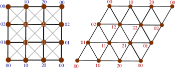
Figure 1: Square lattice extended coupling geometry with interactions with nearest and next-nearest neighbors (left) and the periodic triangular lattice and labeling scheme (right)

In Section IV, we examine two dimensional lattices such as those shown in Fig. 1 with motion confined to the crystal plane, finding the very slow (i.e. logarithmic) loss of crystalline order anticipated for two dimensional crystals. On the other hand, for a two dimensional crystal embedded in three dimensions, it is important to consider transverse perturbations tending to push atoms out of the plane. We find that in the absence of binding to a substrate, two dimensional crystals are much less able to resist extraplanar distortions than fluctuations which are confined to the lattice plane.

In Section V, we examine dual-layer systems where coupling between the crystal planes imparts local stability with respect to extra-planar variations of atomic positions in a caricature of physical systems (e.g. sheets of graphene) which have a finite thickness, and would be imbued with local stiffness. We find for two distinct locally rigid dual-layer geometries similar rapid divergences of mean square displacements as the crystal is made larger, corresponding to thermally induced rippling of the crystal, and scaling linearly with the size of the system. Analysis of the density of vibrational states reveals that the length scale of the random undulations increases with the size of the system with strong long wavelength contributions. On the other hand coupling to a flat substrate, however weak, places an asymptotic upper bound on the ripple amplitudes and also limits the average wavelength of thermally induced undulations.

II Calculation methods and Monte-Carlo Simulation Results

We examine thermodynamic properties (e.g. the mean square deviations of atoms about equilibrium positions) for crystals with short range bonding in the regime where bonds remain intact and thermally induced lengthening and shortening of bonds is small relative to the unperturbed, or equilibrium, bond length. With individual bonds varying only slightly in length, it is appropriate to model the bonds as harmonic potentials so the couplings between neighboring atoms are effectively treated as springs connecting the two particles. It is important to note that although we neglect anharmonic effects from the bonds, the noncollinearity of bonds in the crystal geometry may in principle introduce anharmonic terms in the Hamiltonian. Nevertheless, at temperatures near and below the melting point, many scenarios are amenable to the harmonic approximation where the neglect of anharmonicities (whether intrinsic or geometric) has a small impact on the accuracy of the calculation. Analytical results obtained in the context of the harmonic approximation are validated in the cases we consider by good agreement with Monte-Carlo calculations where the anharmonic characteristics of the bonding stemming from peculiarities of the lattice geometry are rigorously taken into account.

The Hamiltonian is given by

$$\mathcal{H}=\frac{1}{2}\sum_{i=1}^{N}\sum_{j=1}^{m_{i}}\frac{K_{ij}}{2}\left(l_{ij}-l_{ij}^{0}\right)^{2}$$ (1)

where $l_{ij}^{0}$ is the equilibrium energetically favored bond length and $l_{ij}$ is the instantaneous separation between atoms $i$ and $j$. The outer sum is over the atoms in the (finite) crystal, and the inner sum is over the neighbors associated with the atom indexed by the label $i$. The additional factor of 1/2 is included to compensate for double counting of bonds. The constant $K_{ij}$ is the second derivative of the interatomic potential $V_{ij}(r)$ at the equilibrium separation $l_{ij}^{0}$.

We develop the harmonic approximation directly from the bond length $l_{ij}=\sqrt{(x_{i}-x_{j})^{2}+(y_{i}-y_{j})^{2}+(z_{i}-z_{j})^{2}}$ For the $x$ coordinates, it is convenient to write, for example, $x_{i}=x_{i}^{0}+\delta_{i}^{x}$ where $x_{i}^{0}$ is the equilibrium coordinate and $\delta_{i}^{x}$ is the shift about equilibrium. We operate in the same way for the $y$ and $z$ coordinates, finding

$$l_{ij}=\sqrt{\begin{array}[]{c}(\Delta_{ij}^{0x}+\delta_{i}^{x}-\delta_{j}^{x})^{2}+(\Delta_{ij}^{0y}+\delta_{i}^{y}-\delta_{j}^{y})^{2}\\ +(\Delta_{ij}^{0z}+\delta_{i}^{z}-\delta_{j}^{z})^{2}\end{array}},$$ (4)

where $\Delta_{ij}^{0x}\equiv(x_{i}^{0}-x_{j}^{0})$, $\Delta_{ij}^{0y}\equiv(y_{i}^{0}-y_{j}^{0})$, and $\Delta_{ij}^{0z}\equiv(z_{i}^{0}-z_{j}^{0})$. One may develop the harmonic approximation by expanding terms such as $(l_{ij}-l_{ij}^{0})^{2}$ to quadratic order in the shift differences $(\delta_{i}^{x}-\delta_{j}^{x})$, $(\delta_{i}^{y}-\delta_{j}^{y})$, and $(\delta_{i}^{z}-\delta_{j}^{z})$. The result will be $(l_{ij}-l_{ij}^{0})\approx\left[\hat{\Delta}_{ij}\cdot\left(\vec{\delta}_{i}-\vec{\delta}_{j}\right)\right]^{2}$, where $\hat{\Delta}_{ij}$ is a unit vector formed from $\vec{\Delta}_{ij}=(\Delta_{ij}^{0x},\Delta_{ij}^{0y},\Delta_{ij}^{0z})$.The terms $\vec{\delta}_{i}$ and $\vec{\delta}_{j}$ are vector atomic displacements such that, e.g., $\vec{\delta}_{i}=(\delta_{i}^{x},\delta_{i}^{y},\delta_{i}^{z})$. A salient characteristic of the bond energy is its dependence on the differences of the coordinate shifts (e.g. $\delta_{i}^{x}-\delta_{j}^{x}$ for the $x$ direction) instead of $\delta_{i}^{x}$, $\delta_{i}^{y}$, and $\delta_{i}^{z}$ by themselves, a condition which under many circumstances permits the neglect of anharmonicities due to bond non-collinearity.

In the harmonic approximation, the lattice energy due to deviations from equilibrium positions will be

$$\mathcal{H}^{\mathrm{Har}}=\frac{1}{2}\sum_{i=1}^{N}\sum_{j=1}^{m_{i}}\frac{K_{ij}}{2}\left[\hat{\Delta}_{ij}\cdot\left(\vec{\delta}_{i}-\vec{\delta}_{j}\right)\right]^{2}$$ (5)

On expanding, one obtains a quadratic expression mixing the displacements

$$\mathcal{H}^{\mathrm{Har}}\!=\!\sum_{i=1}^{N}\sum_{j=1}^{m_{i}}\!\tfrac{K_{ij}}{4}\!\left[\begin{array}[]{ccc}\delta_{i}^{x}&\delta_{i}^{y}&\delta_{i}^{z}\end{array}\!\right]\!\!\!\left[\!\begin{array}[]{ccc}a_{xx}&a_{xy}&a_{xz}\\ a_{yx}&a_{yy}&a_{yz}\\ a_{zx}&a_{zy}&a_{zz}\end{array}\!\right]\!\!\!\!\left[\!\begin{array}[]{c}\delta_{j}^{x}\\ \delta_{j}^{y}\\ \delta_{j}^{z}\end{array}\!\right]$$ (13)

Diagonalizing the appropriate matrix yields 3$N$ eigenvectors, taken to be normalized. Each of the set of 3N eigenvectors has a component for the individual degrees of freedom in the crystal lattice, permitting the lattice Hamiltonian to be written in decoupled form as

$$\mathcal{H}^{\mathrm{Har}}=\frac{K}{2}\sum_{\alpha=1}^{3N}\lambda_{\alpha}c_{\alpha}^{2}$$ (14)

with eigenvector expansion coefficients $c_{\alpha}$ and eigenvalues $\lambda_{\alpha}$; the parameter $K$ is the “primary” harmonic constant, which is taken to be the nearest neighbor intra-planar coupling constant in schemes, such as extended models with multiple coupling constants. The eigen-modes are independently excited by thermal fluctuations, and thermodynamic equilibrium observables may be calculated by evaluating Gaussian integrals. As an example, the thermally averaged mean square fluctuation per atomic species $\langle\delta_{\textrm{RMS}}\rangle$ is (first moments of the coordinate shifts such as $\langle\delta_{i}^{x}\rangle$ vanish in the thermal average and do not appear in the expression below)

$$\langle\delta_{\textrm{RMS}}\rangle^{2}=\tfrac{1}{N}\sum_{i=1}^{N}\langle(\delta_{i}^{x})^{2}+(\delta_{i}^{y})^{2}+(\delta_{i}^{z})^{2}\rangle$$ (15)

Indexing the eigenvectors with the label $\alpha$ and noting, e.g., that $\delta_{i}^{x}=\displaystyle{\sum_{\alpha=1}^{3N}}c_{\alpha}v_{\alpha}^{ix}$, we see that the total square of the instantaneous fluctuations per particle is

$$\delta_{\mathrm{RMS}}=\tfrac{1}{N}\sum_{i=1}^{N}\!\sum_{\alpha=1}^{3N}\sum_{\alpha^{{}^{\prime}}=1}^{3N}\left[c_{\alpha}c_{\alpha^{{}^{\prime}}}(v_{\alpha}^{ix}v_{\alpha^{{}^{\prime}}}^{ix}+v_{\alpha}^{iy}v_{\alpha^{{}^{\prime}}}^{iy}+v_{\alpha}^{iz}v_{\alpha^{{}^{\prime}}}^{iz})\right]$$ (16)

In calculating the thermal average the term $c_{\alpha}c_{\alpha^{{}^{\prime}}}$ will be as often negative as positive when $\alpha\neq\alpha^{{}^{\prime}}$, and there will only be a non-zero contribution to $\langle\delta_{\mathrm{RMS}}\rangle^{2}$ if $\alpha=\alpha^{{}^{\prime}}$. Hence, the double sum enclosed in square brackets will collapse to a single sum, and the calculation is reduced to the thermal average

$$\langle\delta_{\mathrm{RMS}}\rangle^{2}=\tfrac{1}{N}\sum_{\alpha=1}^{3N}\langle c_{\alpha}^{2}\rangle\sum_{i=1}^{N}\left[(v_{\alpha}^{ix})^{2}+(v_{\alpha}^{iy})^{2}+(v_{\alpha}^{iz})^{2}\right]$$ (17)

The eigenvector normalization condition gives

$$\sum_{i=1}^{N}\left[(v_{\alpha}^{ix})^{2}+(v_{\alpha}^{iy})^{2}+(v_{\alpha}^{iz})^{2}\right]=1,$$ (18)

and hence $\langle\delta_{\mathrm{RMS}}\rangle^{2}$ appears simply as

$$\langle\delta_{\mathrm{RMS}}\rangle^{2}=\tfrac{1}{N}\sum_{\alpha=1}^{3N}\langle(c_{\alpha})^{2}\rangle$$ (19)

The partition function $Z$ may be calculated with the aid of $\int_{-\infty}^{\infty}e^{-\sigma q^{2}}dq=(\pi/\sigma)^{1/2}$, and one has a product of decoupled Gaussian integrals, which may be written as

$$Z=\prod_{\alpha=1}^{3N}\int_{-\infty}^{\infty}e^{-K\beta\lambda_{\alpha}c_{\alpha}^{2}/2}dc_{\alpha}$$ (20)

with $\beta=1/k_{\mathrm{B}}$, $k_{\mathrm{B}}$ the Boltzmann constant, and the temperature $T$ is given in Kelvins. For the sake of convenience, units are chosen such that the lattice constant $a$ is equal to unity, and a reduced temperature is defined with $t\equiv k_{\mathrm{B}}T/K$. Evaluating the integrals in the product given in Eq. 20 yields for $Z$

$$Z=\prod_{\alpha=1}^{3N}\left(\frac{2\pi t}{\lambda_{\alpha}}\right)^{1/2}$$ (21)

The thermally averages mean square displacement may be written in terms of a thermal logarithmic derivative of $Z$, and in particular, one finds

$$\langle\delta_{\mathrm{RMS}}\rangle^{2}=t^{2}\frac{d}{dt}\textrm{Ln}(Z)=\sum_{\alpha=1}^{3N}\lambda_{\alpha}^{-1}t$$ (22)

Hence, the thermally averaged mean square deviation from equilibrium may be written as the square root of a sum over eigenvalue reciprocals.

$$\langle\delta_{\mathrm{RMS}}\rangle=t^{1/2}\sqrt{\sum_{\alpha=1}^{3N}\lambda_{\alpha}^{-1}}$$ (23)

Zero eigenvalues would lead to a diverging expression, but eigenvalues which are strictly equal to zero are artifacts of periodic boundary conditions, correspond to global translations of the crystal lattice, and are excluded from the sum. The dependence on reduced temperature consists of a $t^{1/2}$ factor. To concentrate on characteristics specific to a lattice geometry and its coupling scheme, as well as trends with respect to system size $L$, the normalized mean square displacement $\delta_{\mathrm{RMS}}^{{n}}$ will often be discussed in lieu of the full temperature dependent quantity.

In the case of a periodic regular crystal lattice, it is useful exploit translational invariance, which will lead to exact expressions for the vibrational mode eigenstates and frequencies for periodic crystals (or at the very least yielding a small matrix which may be diagonalized analytically or by numerical means if necessary) if atomic displacements are written in terms of the corresponding Fourier components.

Using Monte Carlo calculations to sample thermodynamic quantities incorporates anharmonic effects in a rigorous manner, providing a means of assessing the validity of the harmonic approximation. We employ the Metropolis technique Metropolis (1953) to introduce random displacements and sample the distribution corresponding to thermal equilibrium. We follow the standard Metropolis prescription, where an attempted random displacement with an associated energy shift $\Delta E$ is accepted with probability $e^{-\Delta E/k_{\mathrm{B}}T}$ if $\Delta E>0$ and the Monte Carlo move is invariably accepted for cases in which $\Delta E<0$.

In calculating thermodynamic quantities, we operate in terms of Monte Carlo sweeps where a sweep, on average, consists of an attempt to move each atom in the crystal with the acceptance of the move subject to the Metropolis condition. In the calculations, the sampling of thermodynamic quantities is postponed until the completion of the first 25% of the total number of sweeps to eliminate bias from the initial conditions, which are not typical thermal equilibrium configurations for the system. To reduce errors due to statistical fluctuations in the Monte Carlo simulation and obtain several digits of accuracy in the results, we conduct at least $5\times 10^{5}$ sweeps. Figure 2 (for the square lattice with an extended coupling scheme) and Figure 3 (for the triangular lattice geometry) show mean square deviation curves for various temperatures ranging from temperatures an order of magnitude smaller than $T_{\mathrm{3D}}^{\mathrm{L}}$ to temperatures on par with the Lindemann criterion result for the melting temperature of the corresponding three dimensional system. The solid lines correspond to analytical results, while the symbols are RMS values obtained with Monte Carlo calculations.

The curves show very good agreement between the Monte Carlo data and analytical results over a wide range of temperatures and system sizes, and deviations are primarily mild statistical errors (on the order of one part in $10^{3}$) in the Monte Carlo calculations.

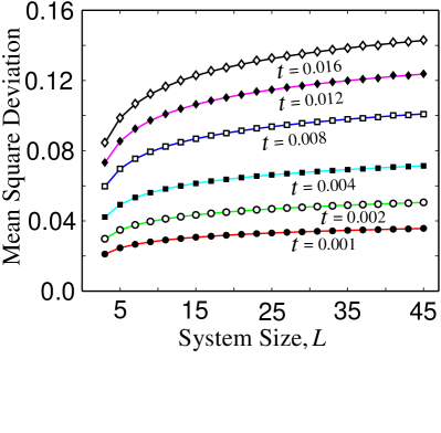
Figure 2: Graph of the RMS fluctuation about equilibrium versus systems size $L$ for various values of the reduced temperature $t$ for the square lattice with next-nearest neighbor couplings. The solid lines are analytic results obtained in the harmonic approximation, and symbols are results from Monte Carlo calculations.

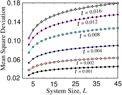
Figure 3: Graph of the RMS fluctuation about equilibrium versus systems size $L$ for various values of the reduced temperature $t$ for the triangular lattice. The solid lines are analytic results obtained in the harmonic approximation, and symbols are results from Monte Carlo calculations.

Figure 4: Illustration of the simple cubic, nonrigid structure and rigidity gained by incorporating next nearest-neighbor couplings as shown in the image to the right.

III Rigid and Non-Rigid Three Dimensional lattices

To establish a temperature scale for the two dimensional systems, where long-range crystalline order is not expected to exist at temperatures above 0K, we first examine three dimensional lattices, which may exhibit long-range positional order at finite temperature if the lattice is suitably rigid. As a preliminary step, we perform an analysis similar to the Lindemann treatment where an atom in a simple cubic geometry is coupled to six nearest neighbors. Since we do not take into account the motion of neighboring atoms, we take their displacements to be zero; certainly the excursions of neighboring atoms would average to zero, although to be precise, one would need to take into account cooperative effects of the atomic motions of the neighbors.

The lattice energy has the form

$$\hat{h}_{\mathrm{L}}^{\mathrm{3D}}=\frac{K}{2}\left(\begin{array}[]{c}\Delta_{x_{+}}^{2}+\Delta_{x_{-}}^{2}+\Delta_{y_{+}}^{2}+\Delta_{y_{-}}^{2}+\Delta_{z_{+}}^{2}+\Delta_{z_{-}}^{2}\end{array}\right)$$ (25)

where, for example, $\Delta_{x_{+}}$ is the shift in length of the bond to the nearest neighbor in the positive $\hat{x}$ direction. Applying the harmonic approximation and taking the atomic shifts to be $\left\{\delta_{x},\delta_{y},\delta_{z}\right\}$, the energy becomes

$$\hat{h}_{\mathrm{L}}^{\mathrm{3D}}=K\left[\delta_{x}^{2}+\delta_{y}^{2}+\delta_{z}^{2}\right]$$ (26)

In the calculation of $\delta_{\mathrm{RMS}}$, the partition function has the form

$$Z=\int^{\infty}_{-\infty}\int^{\infty}_{-\infty}\int^{\infty}_{-\infty}e^{-\tfrac{\delta_{x}^{2}+\delta_{y}^{2}+\delta_{z}^{2}}{t}}d\delta_{x}d\delta_{y}d\delta_{z}$$ (27)

From the Gaussian integration, we find $Z=(\pi t)^{3/2}$. The RMS displacement will be $\langle r^{2}\rangle^{1/2}$ where

$$\langle r^{2}\rangle=t^{2}\tfrac{d}{dt}\textrm{Ln}(Z)=3t/2$$ (28)

Hence, the thermally averaged mean square shift is $(3t/2)^{1/2}$. The Lindemann criterion places the melting temperature at a temperature high enough that the mean square deviation $\delta_{\mathrm{RMS}}$ reaches a tenth of a lattice constant, which corresponds to $t_{\mathrm{L}}^{\mathrm{3D}}=\tfrac{2}{3}(10^{-2})$, a reduced temperature on the order of $0.01$.

If correlations among atoms are taken into account, next-nearest neighbor couplings become crucial to imparting local stiffness and maintaining long-range crystalline order. To see how rigidity is an important factor, we calculate the RMS displacements for a simple cubic lattice where only couplings between nearest neighbors are taken into account. The energy stored in the lattice will be

$$E=\frac{K}{2}\sum_{i,j,k=0}^{n-1}\left[\!\!\begin{array}[]{c}(\delta_{i+1jk}^{x}-\delta_{ijk}^{x})^{2}+(\delta_{ij+1k}^{y}-\delta_{ijk}^{y})^{2}\\ +(\delta_{ijk+1}^{z}-\delta_{ijk}^{z})^{2}\end{array}\!\!\right]$$ (31)

where a periodic geometry is assumed, and the counting factor of $1/2$ does not appear since the sum has been constructed to avoid redundancies. If we use the transformations

$$\delta_{ijk}^{x}=\sum_{k_{x}k_{y}k_{z}}\delta_{\bf{k}}^{x}e^{I(k_{x}i+k_{y}j+k_{z}k)}$$ (32)

where $I$ is the imaginary unit, and similar expressions are used for $\delta_{ijk}^{y}$ and $\delta_{ijk}^{z}$. In terms of the Fourier components, the lattice energy may be written as

$$E=\frac{K}{2}\!\!\sum_{k_{x},k_{y},k_{z}}\left[\!\begin{array}[]{c}(1-\cos k_{x})|\delta_{\bf{k}}^{x}|^{2}\\ +(1-\cos k_{y})|\delta_{\bf{k}}^{y}|^{2}\\ +(1-\cos k_{z})|\delta_{\bf{k}}^{z}|^{2}\end{array}\!\right]$$ (36)

The $x$, $y$, and $z$ degrees of freedom $\delta_{\bf{k}}^{x}$, $\delta_{\bf{k}}^{y}$, and $\delta_{\bf{k}}^{z}$ automatically decouple. The normalized mean square deviation is $\sqrt{\sum_{\alpha}\lambda_{\alpha}^{-1}}$, where the sum is restricted to non-zero eigenvalues. We identify three eigenvalues, $\lambda_{\bf{k}}^{(1)}=2(1-\cos k_{x})$, $\lambda_{\bf{k}}^{(2)}=2(1-\cos k_{y})$, and $\lambda_{\bf{k}}^{(3)}=2(1-\cos k_{z})$ for each wave vector $\left\{k_{x},k_{y},k_{z}\right\}$ As can be seen in Figure, the mean square fluctuation about equilibrium positions grows very rapidly with increasing system size. The divergence in the RMS displacements is a consequence of the lack of rigidity of the simple cubic geometry, which facilitates the destruction of long range crystalline order by thermal fluctuations. However, next-nearest neighbor couplings make the lattice rigid, and are very effective in suppressing fluctuations about equilibrium and establishing long-range crystalline order for the simple cubic lattice.

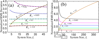
Figure 5: RMS displacements graphed with system size $L$ for various values of $K_{2}$, expressed in units of the nearest-neighbor coupling $K_{1}$. Panel (a) shows a closer view of the $\delta_{\mathrm{RMS}}$ curves over a smaller range of system sizes, and panel (b) is a graph with a broader range of system sizes included in the plot.

Figure 6: RMS displacements graphed as a function of the ratio of next nearest neighbor to nearest neighbor coupling, $K_{2}/K_{1}$. Inset (a) is a graph of the normalized RMS deviation with respect to $\log_{10}(K_{2}/K_{1})$, and inset (b) shows the RMS fluctuations raised to the 1/4 power versus $\log_{10}(K_{2}/K_{1})$.

The structure of the eigenvalue density states profile has informative characteristics particular to the lattice geometry from which it is obtained, and the density of states is calculated for many of the systems we report on. We achieve the thermodynamic in a genuine sense by not restricting $k_{x}$, $k_{y}$, and $k_{z}$ to discrete values as is done for finite systems. The density of states is built up by Monte Carlo sampling in which the wave-vector components are each generated independently from a uniform random distribution. To obtain good statistics, at least on the order of $2\times 10^{8}$ eigenvalues are sampled in constructing the DOS. The same Monte Carlo sampling procedure is used to calculate the $\delta_{\mathrm{RMS}}$ values shown in Fig. 6, and thereby completely remove any bias from finite size effects. The density of states corresponding to the simple cubic system (shown in the graph in Fig. 7) is consistent with the divergence of the RMS fluctuations with increasing system size. The bimodal structure is sharply peaked in the low and high eigenvalue regimes, with the former contributing to the steady rise of $\delta_{\mathrm{RMS}}$ with increasing system size $L$.

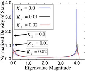
Figure 7: Normalized Eigenvalue Density of States for the simple cubic system for an extended coupling scheme with $K_{2}=\left\{0.0,0.01,0.02\right\}$ with a sampling of $2.4\times 10^{8}$ eigenvalues.

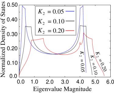
Figure 8: Normalized Eigenvalue Density of States for the simple cubic system for an extended coupling scheme with $K_{2}=\left\{0.05,0.10,0.20\right\}$ with a sampling of $2.4\times 10^{8}$ eigenvalues.

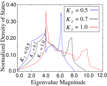
Figure 9: Normalized Eigenvalue Density of States for the simple cubic system with coupling for an extended coupling scheme with $K_{2}=\left\{0.5,0.7,1.0\right\}$ with a sampling of $2.4\times 10^{8}$ eigenvalues.

In the extended coupling scheme in the simple cubic geometry, the energy stored in the lattice is

$$E\!=\!\frac{K_{1}}{2}\!\!\!\!\sum_{i,j,k=0}^{n-1}\!\left(\!\!\!\begin{array}[]{c}\left\{\!\!\!\begin{array}[]{l}[\hat{x}\!\cdot\!(\vec{\delta}_{i+1jk}\!-\!\vec{\delta}_{ijk})]^{2}\!+\![\hat{y}\!\cdot\!(\vec{\delta}_{ij+1k}\!-\!\vec{\delta}_{ijk})]^{2}\\ \!+\![\hat{z}\!\cdot\!(\vec{\delta}_{ijk+1}\!-\!\vec{\delta}_{ijk})]^{2}\end{array}\!\!\right\}\\ \!\!\!+\kappa_{2}\!\left\{\!\!\!\begin{array}[]{l}\left[\frac{1}{\sqrt{2}}(\hat{x}+\hat{y})\cdot(\vec{\delta}_{i+1j+1k}-\vec{\delta}_{ijk})\right]^{2}\!+\!\\ \left[\frac{1}{\sqrt{2}}(\hat{x}\!-\!\hat{y})\!\cdot\!(\vec{\delta}_{i+1j-1k}\!-\!\vec{\delta}_{ijk})\right]^{2}\!\!+\!\\ \left[\frac{1}{\sqrt{2}}(\hat{y}\!+\!\hat{z})\!\cdot\!(\vec{\delta}_{ij+1k+1}\!-\!\vec{\delta}_{ijk})\right]^{2}\!\!+\!\\ \left[\frac{1}{\sqrt{2}}(\hat{y}\!-\!\hat{z})\!\cdot\!(\vec{\delta}_{ij+1k-1}\!-\!\vec{\delta}_{ijk})\right]^{2}\!\!+\!\\ \left[\frac{1}{\sqrt{2}}(\hat{x}\!+\!\hat{z})\!\cdot\!(\vec{\delta}_{i+1jk+1}\!-\!\vec{\delta}_{ijk})\right]^{2}\!\!+\!\\ \left[\frac{1}{\sqrt{2}}(\hat{x}\!-\!\hat{z})\!\cdot\!(\vec{\delta}_{i+1jk-1}\!-\!\vec{\delta}_{ijk})\right]^{2}\end{array}\!\!\!\!\right\}\end{array}\!\!\!\!\right)$$ (47)

where $K_{1}$ is the coupling to nearest neighbors, $K_{2}$ is the coupling to next-nearest neighbors, and $\kappa_{2}\equiv K_{2}/K_{1}$ is the ratio of the next-nearest and nearest neighbor coupling constants. In terms of Fourier components, one has

$$E\!=\!\frac{K_{1}}{2}\!\!\sum_{\bf{k}}\!\!\left(\!\!\!\begin{array}[]{l}\left\{\!\!\begin{array}[]{l}\!(2\!-\!2\cos k_{x})\lvert\delta_{\bf{k}}^{x}\rvert^{2}\!+\!(2-2\cos k_{y})\lvert\delta_{\bf{k}}^{y}\rvert^{2}\\ \!+\!(2\!-\!2\cos k_{z})\lvert\delta_{\bf{k}}^{z}\rvert^{2}\end{array}\!\!\right\}\!+\!\\ \\ \!\kappa_{2}\!\left\{\!\!\begin{array}[]{l}\left[2\!-\!\cos k_{x}\cos k_{y}\!-\!\cos k_{x}\cos k_{z}\right]\!\lvert\delta_{\bf{k}}^{x}\rvert^{2}\!+\!\\ \left[2\!-\!\cos k_{x}\cos k_{y}\!-\!\cos k_{y}\cos k_{z}\right]\!\lvert\delta_{\bf{k}}^{y}\rvert^{2}\!+\!\\ \left[2\!-\!\cos k_{y}\cos k_{z}\!-\!\cos k_{x}\cos k_{z}\right]\!\lvert\delta_{\bf{k}}^{z}\rvert^{2}\!+\!\\ \sin k_{x}\sin k_{y}(\delta_{\bf{k}}^{x}\delta_{\bf{k}}^{*y}+\delta_{\bf{k}}^{*x}\delta_{\bf{k}}^{y})+\\ \sin k_{y}\sin k_{z}(\delta_{\bf{k}}^{y}\delta_{\bf{k}}^{*z}+\delta_{\bf{k}}^{*y}\delta_{\bf{k}}^{z})+\\ \sin k_{z}\sin k_{x}(\delta_{\bf{k}}^{z}\delta_{\bf{k}}^{*x}+\delta_{\bf{k}}^{*z}\delta_{\bf{k}}^{x})\end{array}\!\!\!\right\}\end{array}\!\!\!\!\!\right)$$ (59)

with $\bf{k}$ indicating the wave-vector with components $k_{x}$, $k_{y}$, and $k_{z}$, and again $\kappa_{2}=K_{1}/K_{2}$. The eigenvalues are hence obtained by diagonalizing the 3$\times$3 matrix

$$2\!\!\left[\!\!\!\begin{array}[]{ccc}\left(\!\!\begin{array}[]{c}2\!-\!\cos k_{x}\cos k_{y}\\ \!-\!\cos k_{x}\cos k_{z}\end{array}\!\!\!\right)\!\!&\!\!\kappa_{2}\sin k_{x}\sin k_{y}\!\!\!&\!\!\!\kappa_{2}\sin k_{x}\sin k_{z}\\ \\ \kappa_{2}\sin k_{x}\sin k_{y}\!\!\!&\!\!\!\left(\!\!\begin{array}[]{c}2\!-\!\cos k_{y}\cos k_{z}\\ \!-\!\cos k_{z}\cos k_{x}\end{array}\!\!\!\right)\!\!\!&\!\!\!\kappa_{2}\sin k_{y}\sin k_{z}\\ \\ \kappa_{2}\sin k_{z}\sin k_{x}\!\!\!&\!\!\!\kappa_{2}\sin k_{z}\sin k_{y}\!\!\!&\!\!\!\left(\!\!\begin{array}[]{c}2\!-\!\cos k_{z}\cos k_{y}\\ \!-\!\cos k_{z}\cos k_{x}\end{array}\!\!\!\right)\end{array}\!\!\!\right]$$ (71)

Although solving the cubic characteristic equation will yield analytical expressions for the eigenvalues, the result is cumbersome, and we instead use standard algorithms for the diagonalization of a symmetric matrix to efficiently obtain the eigenvalues numerically.

The eigenvalues determined in this manner are used to calculate the means square atomic fluctuations, and the results are shown in Figure 5, where $\delta_{\mathrm{RMS}}$ is graphed with respected to $L$ for a range of the next to nearest neighbor coupling strength ratio $\kappa_{2}=K_{2}/K_{1}$. Whereas the mean square displacement steadily rises with system size when $\kappa_{2}=0$ (i.e with only nearest-neighbor couplings active), the curves behave very differently for nonzero $\kappa_{2}$, ultimately saturating with increasing $L$. The stabilization of $\delta_{\mathrm{RMS}}$ in the thermodynamic limit indicates the presence of intact long-range crystalline order. In the case of $\kappa_{2}=0$, the mean square deviation steadily diverges with increasing $L$. The same divergence with only nearest-neighbor interactions taken into a account occurs whether one is considering the simple cubic structure, a square lattice, or a linear chain. Hence, in some lattice geometries, having a three dimensional structure may be insufficient to stabilize long-range order if an extended coupling scheme is not taken into consideration.

By switching on and varying the strength of the next-nearest coupling $K_{2}$, one sees the appearance of long-range crystalline order as the cubic system is made increasingly rigid. In Fig. 6 the mean square displacement is shown graphed versus the coupling ratio $K_{2}/K_{1}$. The tendency for atoms to be driven from their positions in the lattice does increase as $K_{2}$ is shut off, but the divergence occurs at a slow rate. Inset (a) is a graph of $\delta_{\textrm{RMS}}$ versus the logarithm of $K_{2}/K_{1}$. While the concavity of the curve indicates a somewhat more rapid than logarithmic divergence, a semi-logarithmic plot of $\delta_{\mathrm{RMS}}$ (i.e. as shown in inset (b) of Fig. 6) shows an approximately linear scaling of $\delta_{\mathrm{RMS}}^{1/4}$ with the logarithm of the system size, still a relatively slow divergence, albeit somewhat more rapid than a simple logarithmic divergence. Hence, the next-nearest neighbor couplings in the extended coupling simple cubic model are very effective in restoring long-range crystalline order.

Trends in the eigenvalue density of states profile with increasing $K_{2}/K_{1}$ to next-nearest neighbors are shown in in Fig. 7, Fig. 8, Fig. 9. The almost immediate retreat of the low and high frequency peaks toward the center is consistent with the effectiveness of an extended coupling scheme in stabilizing long-range crystalline order even for very small values of the ratio $\kappa_{2}=K_{2}/K_{1}$. The DOS profile has a simple structure for small $\kappa_{2}<0.1$, while intermediate $\kappa_{2}$ values are associated with a richer density of states curve which changes rapidly as the coupling ratio is increased further.

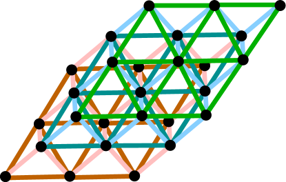
Figure 10: Illustration of the tetrahedral lattice geometry

As in the case of the cubic lattice with the extended coupling scheme, we may calculate the lattice energy in the harmonic approximation for the tetrahedral lattice, which is

$$E=\!\frac{K}{2}\!\!\sum_{i,j,k=0}^{n-1}\!\!\left(\!\!\begin{array}[]{l}\left[\vec{x}\!\cdot\!(\vec{\delta}_{i+1jk}\!-\!\vec{\delta}_{ijk})\right]^{2}+\\ \left[\!\left(\!\frac{1}{2}\hat{x}\!+\!\frac{\sqrt{3}}{2}\hat{y}\!\right)\!\cdot\!(\vec{\delta}_{ij+1k}\!-\!\vec{\delta}_{ijk})\!\right]^{2}\!+\!\\ \left[\!\left(\!\frac{1}{2}\hat{x}\!-\!\frac{\sqrt{3}}{2}\hat{y}\!\right)\!\cdot\!(\vec{\delta}_{i+1j-1k}\!-\!\vec{\delta}_{ijk})\!\right]^{2}\!+\!\\ \left[\!\left(\!\frac{1}{2}\hat{x}\!+\!\frac{1}{2\sqrt{3}}\hat{y}\!+\!\sqrt{\frac{2}{3}}\hat{z}\!\right)\!\cdot\!(\vec{\delta}_{ijk+1}\!-\!\vec{\delta}_{ijk})\!\right]^{2}\!+\!\\ \left[\!\left(\!-\frac{1}{2}\hat{x}\!+\!\frac{1}{2\sqrt{3}}\hat{y}\!+\!\sqrt{\frac{2}{3}}\hat{z}\!\right)\!\cdot\!(\vec{\delta}_{i-1jk+1}\!-\!\vec{\delta}_{ijk})\!\right]^{2}\\ \!+\!\left[\left(-\frac{1}{\sqrt{3}}\hat{y}\!+\!\sqrt{\frac{2}{3}}\hat{z}\!\right)\cdot(\vec{\delta}_{ij-1k+1}\!-\!\vec{\delta}_{ijk})\!\right]^{2}\end{array}\!\!\!\right)$$ (78)

where there is only one coupling constant $K$ since bonds are considered between nearest neighbors only, the tedrahedral geometry being intrinsically rigid, and we have used the fact that the altitude of a tetrahedron is $\sqrt{\tfrac{2}{3}}$ times the lattice constant. The energy may be expressed in terms of Fourier components, and one has the task of diagonalizing the $3\times 3$ matrix

$$\left[\!\!\!\!\!\begin{array}[]{ccc}\left(\!\!\!\!\begin{array}[]{c}4-2\cos k_{x}-\\ \frac{1}{2}(\cos k_{y}\!+\!\cos k_{z})\\ -\frac{1}{2}\cos(k_{y}\!-\!k_{x})\\ -\frac{1}{2}\cos(k_{z}\!-\!k_{y})\end{array}\!\!\!\!\right)\!\!\!\!\!\!\!&\tfrac{\sqrt{3}}{2}\!\!\left(\!\!\!\begin{array}[]{c}\cos(k_{y}\!-\!k_{x})\\ -\cos k_{y}\end{array}\!\!\!\right)\!\!\!\!\!&\sqrt{\tfrac{2}{3}}\!\!\left(\!\!\!\begin{array}[]{c}\cos(k_{z}-k_{x})\\ -\cos k_{z}\end{array}\!\!\!\right)\\ \\ \tfrac{\sqrt{3}}{2}\!\!\left(\!\!\!\begin{array}[]{c}\cos(k_{y}\!-\!k_{x})\\ -\cos k_{y}\end{array}\!\!\!\right)\!\!\!\!\!\!\!&\left(\!\!\!\!\begin{array}[]{c}4-\tfrac{3}{2}\cos k_{y}\\ -\tfrac{3}{2}\cos(k_{y}\!-\!k_{x})\\ -\tfrac{1}{6}\cos k_{z}-\\ \tfrac{2}{3}\cos(k_{z}\!-\!k_{y})\\ -\tfrac{1}{6}\cos(k_{z}\!-\!k_{z})\end{array}\!\!\!\!\right)\!\!\!\!\!&\tfrac{1}{\sqrt{3}}\!\!\left(\!\!\!\begin{array}[]{c}2\cos(k_{z}\!-\!k_{y})\\ -\cos k_{z}-\\ \cos(k_{z}\!-\!k_{x})\end{array}\!\!\!\right)\\ \\ \sqrt{\tfrac{2}{3}}\!\!\left(\!\!\!\begin{array}[]{c}\cos(k_{z}\!-\!k_{x})\\ -\cos k_{z}\end{array}\!\!\!\right)\!\!\!\!\!\!\!&\tfrac{1}{\sqrt{3}}\!\!\left(\!\!\!\begin{array}[]{c}2\cos(k_{z}\!-\!k_{y})\\ -\cos k_{z}-\\ \cos(k_{z}\!-\!k_{x})\end{array}\!\!\!\right)\!\!\!\!\!&\tfrac{4}{3}\!\!\left(\!\!\!\!\begin{array}[]{c}3-\cos k_{z}-\\ \cos(k_{z}\!-\!k_{x})-\\ \cos(k_{z}\!-\!k_{y})\end{array}\!\!\!\!\right)\end{array}\!\!\!\!\right]$$ (110)

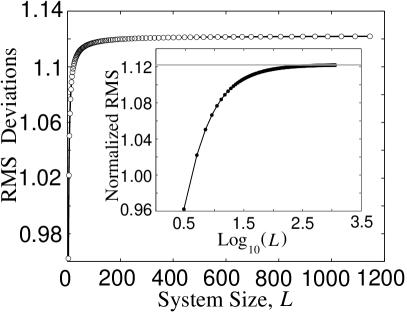
Figure 11: Normalized root mean square (RMS) deviation shown versus $\log_{10}L$ for the three dimensional tetrahedral crystal. The inset is a graph of the normalized RMS deviations, again plotted with respect to $\log_{10}L$, with the horizontal line indicating the extrapolated $\delta_{\mathrm{RMS}}$ in the thermodynamic limit.

The three dimensional tetrahedral lattice is locally stiff even with only nearest-neighbor couplings taken into account, and the rigidity inherent in the tetrahedral lattice geometry is sufficient to preserve long-range crystalline order, as may be seen in Figure 11 which displays the normalized mean square deviation versus the system size $L$. The inset is a semi-logarithmic plot with the horizontal axis extending over three decades of system sizes. The saturation of the normalized RMS displacement with increasing $L$ is evident in both of the graphs, and in the thermodynamic limit, is in the vicinity of $1.12$. With temperature dependence included, one will have $\delta_{\mathrm{RMS}}=1.12t^{1/2}$. Hence, the Lindemann criterion would give $t_{3\mathrm{D}}^{\mathrm{L}}=0.0080$, compatible with the previous estimate which neglected correlations of the atomic displacements from equilibrium.

In inset (a) of Fig. 12, the density of states is shown for the simple cubic lattice geometry with the extended coupling scheme, and for the tetrahedral lattice in inset (b). For both systems, while other details of the density of states profiles differ, the curves tend swiftly to zero in the small eigenvalue regime, a hallmark of intact long range crystalline order in rigid three dimensional lattices.

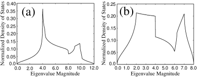
Figure 12: Normalized Eigenvalue Density of States for the cubic crystal with nearest and next-nearest neighbor couplings (a), and the density of states profile for the tetrahedral lattice (b).

IV Intraplanar Motion

We first examine the case where motion perpendicular to the plan is forbidden, and atomic deviations from equilibrium are confined to the lattice plane. We consider various geometries, but first we consider a square (effectively a face-centered system), illustrated in Figure 2, where coupling to the four next nearest neighbors is taken into account. We then consider a locally rigid triangular lattice where each atom interacts with six nearest neighbors. In both the face-centered square and triangular systems, we find a logarithmic divergence with increasing system size in the mean square fluctuations about equilibrium.

For the periodic square geometry with the coupling scheme extended to next-nearest neighbors, the lattice energy to quadratic order is

$$E=\frac{K}{2}\!\!\sum_{i,j=0}^{n-1}\left(\!\!\begin{array}[]{l}\left[\hat{x}\!\cdot\!\left(\vec{\delta}_{i+1j}^{x}\!-\!\vec{\delta}_{ij}^{x}\right)\!\right]^{2}\!+\!\left[\hat{y}\!\cdot\!\left(\vec{\delta}_{ij+1}^{y}\!-\!\vec{\delta}_{ij}^{y}\right)\!\right]^{2}\\ \!+\!\left[\!\tfrac{1}{\sqrt{2}}(\hat{x}\!+\!\hat{y})\!\cdot\!\left(\vec{\delta}_{i+1j+1}^{x}\!-\!\vec{\delta}_{ij}^{x}\right)\!\right]^{2}\\ \!+\!\left[\!\tfrac{1}{\sqrt{2}}(\hat{x}\!-\!\hat{y})\!\cdot\!\left(\vec{\delta}_{i+1j-1}^{x}\!-\!\vec{\delta}_{ij}^{x}\right)\!\right]^{2}\end{array}\!\!\right)$$ (114)

Operating in reciprocal space, one diagonalizes the $2\times 2$ matrix

$$\left[\!\!\begin{array}[]{ll}\left(\!\!\begin{array}[]{c}2-\cos k_{x}\\ -\cos k_{x}\cos k_{y}\end{array}\!\!\right)&\sin k_{x}\sin k_{y}\\ \sin k_{x}\sin k_{y}&\left(\!\!\begin{array}[]{c}2-\cos k_{y}\\ -\cos k_{x}\cos k_{y}\end{array}\!\!\right)\end{array}\!\!\right]$$ (121)

yielding the eigenvalues

$$\lambda^{\pm}_{\bf{k}}=\left(\begin{array}[]{c}4-\cos k_{x}-\cos k_{y}-2\cos k_{x}\cos k_{y}\end{array}\right)$$ (123)

$$\pm\sqrt{\begin{array}[]{c}(\cos k_{x}-\cos k_{y})^{2}+4\sin^{2}k_{x}\sin^{2}k_{y}\end{array}}$$ (125)

In the case of the triangular lattice with six fold coordination, one may also obtain analytical expressions for the mean square deviations. In real space, the harmonic approximation for the energy stored in the lattice is

$$E=\frac{K}{2}\sum_{i,j=0}^{n-1}\left(\!\!\begin{array}[]{l}\left[\hat{x}\!\cdot\!\left(\vec{\delta}_{i+1j}-\vec{\delta}_{ij}\right)\right]^{2}+\\ \left[(\frac{1}{2}\hat{x}+\frac{\sqrt{3}}{2}\hat{y})\!\cdot\!\left(\vec{\delta}_{ij+1}-\vec{\delta}_{ij}\right)\right]^{2}+\\ \left[(\frac{1}{2}\hat{x}-\frac{\sqrt{3}}{2}\hat{y})\!\cdot\!\left(\vec{\delta}_{i+1j-1}-\vec{\delta}_{ij}\right)\right]^{2}\end{array}\!\!\right)$$ (129)

Expressing the displacements in terms of Fourier components, one decouples the $x$ and $y$ degrees of freedom by diagonalizing the matrix

$$\left[\!\!\!\begin{array}[]{cc}\left(\!\!\begin{array}[]{c}3\!-\!2\cos k_{x}\!-\!\\ \tfrac{1}{2}\cos k_{y}\!-\!\tfrac{1}{2}\cos[k_{y}\!-\!k_{x}]\end{array}\!\!\right)\!\!&\tfrac{\sqrt{3}}{2}\left(\cos[k_{y}\!-\!k_{x}]\!-\!\cos k_{y}\right)\\ \\ \tfrac{\sqrt{3}}{2}\left(\cos[k_{y}\!-\!k_{x}]\!-\!\cos k_{y}\right)\!\!&\left(\!\!\begin{array}[]{c}3\!-\!\tfrac{3}{2}\cos k_{y}\\ \!-\!\tfrac{3}{2}\cos[k_{y}\!-\!k_{x}]\end{array}\!\!\right)\end{array}\!\!\!\right]$$ (137)

yields the eigenvalues

$$\!\!\!\!\!\lambda_{\bf{k}}^{\pm}=\left[3-\cos k_{x}-\cos k_{y}-\cos(k_{y}-k_{x})\right]$$ (138)

$$\pm\sqrt{\begin{array}[]{c}\cos^{2}k_{x}\!+\!\cos^{2}k_{y}\!+\!\cos^{2}(k_{y}\!-\!k_{x})\!-\!\cos k_{x}\cos k_{y}\\ \!-\!\cos k_{y}\cos(k_{y}\!-\!k_{x})\!-\!\cos(k_{y}\!-\!k_{x})\cos k_{x}\end{array}}$$ (141)

For convenience in comparison with the analytical results in the harmonic approximation, we consider periodic boundary conditions in the crystal plane. We have also examined anchored lattices, where atoms at the periphery are prevented from moving, while those in the interior are free to move. For both the free and fixed boundary conditions, as in the three dimensional case, we obtain qualitatively similar results, and the same physical phenomena.

In Fig. 13 and Fig. 14, the normalized mean square deviation $\delta^{{n}}_{\mathrm{RMS}}$ is graphed with respect to the system size $L$ for the square lattice in the extended scheme and the triangular lattice, respectively. The overall behavior of the mean square deviations from equilibrium is qualitatively the same for both lattice geometries. In both cases, the main graph is semi-logarithmic with $(\delta_{\mathrm{RMS}}^{{n}})^{2}$ on the ordinate. The traces are linear to a very good approximation for all regimes of $L$ (i.e. for small, moderate, and large) shown, and the linearity is maintained for four decades of system sizes ranging from several to on the order of a few times $10^{4}$ lattice constants.

In Fig. 13 and Fig. 14, inset (a) is a standard plot, and the apparent saturation of the $\delta_{\mathrm{RMS}}^{n}$ curve is a hallmark of the slow loss of long-range crystalline order best seen on a semi-logarithmic graph. Inset (b) in Fig. 13 and Fig. 5 contains as semi-logarithmic plot with $\delta_{\mathrm{RMS}}^{{n}}$ [ instead of $(\delta_{\mathrm{RMS}}^{{n}})^{2}$ ] on the ordinate axis. The curves plotted in this manner are not linear, and it is evident that the divergence of the fluctuations about equilibrium is actually somewhat slower than logarithmic; instead, it is $(\delta_{\mathrm{RMS}}^{{n}})^{2}$ which scales as $\textrm{Ln}(L)$.

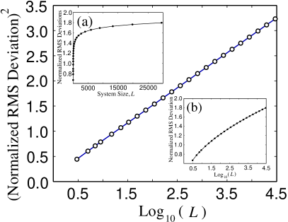
Figure 13: Square of the normalized root mean square (RMS) deviation shown versus $\log_{10}L$ for the square lattice system with extended couplings. The solid line encompassing the open circular symbols is a strictly linear fit. Inset (b) is a semi-logarithmic graph of the normalized RMS deviations, plotted with respect to $\log_{10}L$.

Figure 14: Square of the normalized root mean square (RMS) deviation shown versus $\log_{10}L$ for the triangular lattice. The solid line encompassing the open circular symbols is a strictly linear fit. Inset (a) is a standard plot of the RMS deviation with respect to system size $L$, while inset (b) is a semi-logarithmic graph of the normalized mean square deviations, plotted with respect to $\log_{10}L$.

As in the case of the three dimensional systems, it is informative to examine the density of states, shown in the graph of Fig. 15 for the square lattice in the extended coupling scheme in panel (a) and the triangular lattice in panel (b) of Fig. 15. Again, while details of the density of states profiles shown are peculiar to the lattice under consideration, the behavior in the regime of low eigenvalues is quite similar, and both curves tend to a finite value instead of dropping swiftly to zero as in the density of states for the rigid three dimensional lattices. The failure of the density of states to vanish in the small eigenvalue limit contributes to the slow divergence of $\delta_{\mathrm{RMS}}$ in $L$.

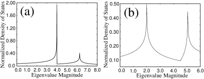
Figure 15: Normalized Eigenvalue Density of States for the face centered square lattice with motion confined to the lattice plane, depicted in panel (a), and for the triangular lattice in panel (b).

V Extra-planar Motion

The locally stiff face-centered square and triangular lattices show the anticipated slow logarithmic divergence in system size. However since laboratory systems often are not vertically constrained, it is important to examine a scenario where motion perpendicular to the plane of the lattice may be considered. There is an important difficulty with single layer systems, in that motion perpendicular to the plane is not hindered since there are no restraining bonds with a directional component transverse to the plane of the layer.

However, by considering dual-layer geometries, it is possible to incorporate local stiffness with respect to perturbations that would push atoms above or below the lattice. We examine analogs of the simple cubic lattice, where we again use an extended coupling scheme to create local stiffness. On the other hand, we also consider a dual-layer tetrahedral lattice. Although the two lattice geometries achieve local stiffness in different ways, the similarities we find in thermodynamic behavior of the mean square atomic fluctuations suggest these characteristics would appear in the generic case as well.

Fig. 16 illustrates the structure of the dual-layer square lattice with an extended coupling scheme; the additional couplings between next nearest neighbors impart local stiffness to the system with respect to perturbations perpendicular to the planes of the square lattices.

Fig. 17 shows how the dual-layer systems is constructed as a caricature of the graphene lattice. The image labeled (a) is a schematic illustration of a single hexagonal cell in a graphene monolayer. The bonding shares similarities with that in a benzene ring with delocalized $\pi$ orbitals forming honeycomb networks of charge density above and below the plane occupied by the carbon atomic nuclei. The superimposed lattice work is a rigid network compatible with the symmetries of the graphene layer and set up to capture the rigidity of the hexagonal cells making up a sheet of graphene. With the honeycomb graphene pattern removed, the remaining lattice geometry and the labeling scheme for the crystal members is shown in Fig. 18.

Figure 16: Illustration of the periodic dual-layer square lattice with nearest and next-nearest neighbor coupling and labeling scheme; blue indices refer to the upper layer, while red indices pertain to the lower plane.

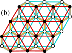
Figure 17: Schematic representation of a coarse-grained super-structure for a graphene sheet

Figure 18: Illustration of the periodic dual-layer triangular lattice and labeling scheme; blue indices refer to the upper layer, while red indices pertain to the lower plane.

With the superscript I representing the lower plane and II indicating the upper plane, the lattice energy in the harmonic approximation is

$$E\!=\!\frac{K}{2}\!\sum_{i,j=0}^{n-1}\!\left(\!\!\begin{array}[]{l}\!\displaystyle\sum_{\alpha=\mathrm{I}}^{\mathrm{II}}\!\left\{\!\!\!\begin{array}[]{l}\left[\hat{x}\!\cdot\!(\vec{\delta}_{i+1j}^{\alpha}-\vec{\delta}_{ij}^{\alpha})\!\right]^{2}\!\!+\!\left[\hat{y}\!\cdot\!(\vec{\delta}_{ij+1}^{\alpha}-\vec{\delta}_{ij}^{\alpha})\!\right]^{2}\\ +\left[\frac{1}{\sqrt{2}}(\hat{x}+\hat{y})\!\cdot\!(\vec{\delta}_{i+1j+1}^{\alpha}-\vec{\delta}_{ij}^{\alpha})\!\right]^{2}+\\ \left[\frac{1}{\sqrt{2}}(\hat{x}-\hat{y})\cdot(\vec{\delta}_{i+1j-1}^{\alpha}\!-\!\vec{\delta}_{ij}^{\alpha})\!\right]^{2}\end{array}\!\!\right\}\\ +\kappa_{z}\left\{\!\!\begin{array}[]{l}\left[\hat{z}\cdot\left(\vec{\delta}_{ij}^{\mathrm{II}}-\vec{\delta}_{ij}^{\mathrm{I}}\right)\right]^{2}\\ \!+\!\left[\tfrac{1}{\sqrt{2}}(\hat{x}\!+\!\hat{z})\!\cdot\!\left(\vec{\delta}_{i+1j}^{\mathrm{II}}\!-\!\vec{\delta}_{ij}^{\mathrm{I}}\right)\right]^{2}\\ \!+\!\left[\tfrac{1}{\sqrt{2}}(-\hat{x}\!+\!\hat{z})\!\cdot\!\left(\vec{\delta}_{i-1j}^{\mathrm{II}}\!-\!\vec{\delta}_{ij}^{\mathrm{I}}\right)\!\right]^{2}\\ \!+\!\left[\tfrac{1}{\sqrt{2}}(\hat{y}\!+\!\hat{z})\!\cdot\!\left(\vec{\delta}_{ij+1}^{\mathrm{II}}\!-\!\vec{\delta}_{ij}^{\mathrm{I}}\right)\!\right]^{2}\\ \!+\!\left[\tfrac{1}{\sqrt{2}}(-\hat{y}\!+\!\hat{z})\!\cdot\!\left(\vec{\delta}_{ij-1}^{\mathrm{II}}\!-\!\vec{\delta}_{ij}^{\mathrm{I}}\right)\!\right]^{2}\end{array}\!\!\right\}\end{array}\!\!\!\!\right)$$ (152)

The corresponding complex Hermitian 6$\times$6 matrix to be diagonalized has the form

$$\left[\!\begin{array}[]{cccccc}a_{\mathrm{I}x\mathrm{I}x}&a_{\mathrm{I}x\mathrm{I}y}&a_{\mathrm{I}x\mathrm{I}z}&a_{\mathrm{I}x\mathrm{II}x}&a_{\mathrm{I}x\mathrm{II}y}&a_{\mathrm{I}x\mathrm{II}z}\\ a_{\mathrm{I}y\mathrm{I}x}&a_{\mathrm{I}y\mathrm{I}y}&a_{\mathrm{I}y\mathrm{I}z}&a_{\mathrm{I}y\mathrm{II}x}&a_{\mathrm{I}y\mathrm{II}y}&a_{\mathrm{I}y\mathrm{II}z}\\ a_{\mathrm{I}z\mathrm{I}x}&a_{\mathrm{I}z\mathrm{I}y}&a_{\mathrm{I}z\mathrm{I}z}&a_{\mathrm{I}z\mathrm{II}x}&a_{\mathrm{I}z\mathrm{II}y}&a_{\mathrm{I}z\mathrm{II}z}\\ a_{\mathrm{II}x\mathrm{I}x}&a_{\mathrm{II}x\mathrm{I}y}&a_{\mathrm{II}x\mathrm{I}z}&a_{\mathrm{II}x\mathrm{II}x}&a_{\mathrm{II}x\mathrm{II}y}&a_{\mathrm{II}x\mathrm{II}z}\\ a_{\mathrm{II}y\mathrm{I}x}&a_{\mathrm{II}y\mathrm{I}y}&a_{\mathrm{II}y\mathrm{I}z}&a_{\mathrm{II}y\mathrm{II}x}&a_{\mathrm{II}y\mathrm{II}y}&a_{\mathrm{II}y\mathrm{II}z}\\ a_{\mathrm{II}z\mathrm{I}x}&a_{\mathrm{II}z\mathrm{I}y}&a_{\mathrm{II}z\mathrm{I}z}&a_{\mathrm{II}z\mathrm{II}x}&a_{\mathrm{II}z\mathrm{II}y}&a_{\mathrm{II}z\mathrm{II}z}\end{array}\!\right]=\left[\!\begin{array}[]{cc}\hat{A}&\hat{B}\\ \hat{B}^{\dagger}&\hat{A}\end{array}\!\right]$$ (161)

where $\hat{A}$ and $\hat{B}$ are $3\times 3$ matrices and $\hat{B}^{\dagger}$ is the Hermitian conjugate of $\hat{B}$. The sub-matrices $\hat{A}$ and $\hat{B}$ are given by

$$\hat{A}=\!K\left[\!\!\!\!\begin{array}[]{ccc}\left(\!\!\begin{array}[]{c}\kappa_{z}\!+\!4\!-\!2\cos k_{x}\\ -2\cos k_{x}\cos k_{y}\end{array}\!\!\!\right)\!\!\!\!&\!\!\!\!2\sin k_{x}\sin k_{y}\!\!\!\!&\!\!\!\!0\\ \\ 2\sin k_{x}\sin k_{y}\!\!\!\!&\!\!\!\!\left(\!\!\begin{array}[]{c}\kappa_{z}\!+\!4\!-\!2\cos k_{y}\\ -2\cos k_{x}\cos k_{y}\end{array}\!\!\!\right)\!\!\!\!&\!\!\!\!0\\ \\ 0\!\!\!\!&\!\!\!\!0\!\!\!\!&3\kappa_{z}\end{array}\!\!\!\right]$$ (171)

where $\kappa_{z}\equiv K_{z}/K$ for $\hat{A}$ and

$$\hat{B}=\!K_{z}\left[\!\!\!\begin{array}[]{ccc}-\cos k_{x}\!&\!0\!&\!\!-i\sin k_{x}\\ \\ 0\!&\!-\cos k_{y}\!&\!-i\sin k_{y}\\ \\ -i\sin k_{x}\!&\!-i\sin k_{y}\!&\!-(1\!+\!\cos k_{x}\!+\!\cos k_{y})\end{array}\!\!\right]$$ (177)

for $\hat{B}$ where the six eigenvalues for each wave-number pair are calculated numerically with code available in the EISPACK linear algebraic library for diagonalizing complex Hermitian matrices.

On the other hand a locally stiff dual-layer system which may be regarded as a section of the three dimensional tetrahedral lattice such that the upper and lower layers are triangular lattices with connections between the layers. The dual-layer lattice structure based on the tetrahedral geometry is illustrated in Figure 18. The vertices of the upper layer are positioned above the centers of the triangles in the lower layer with bonds extending from atoms in the upper layer to each of the corners of the triangle below such that each atom in the dual-layer system is a member of a rigid tetrahedron; the result is a locally stiff layer, as in the dual-layer square lattice extended model, but with a very different geometric structure.

The lattice energy for the dual-layer tetrahedral system to quadratic order in the displacements $\vec{\delta_{ij}}^{\mathrm{I}}$ and $\vec{\delta_{ij}}^{\mathrm{II}}$ has the form

$$E=\frac{K}{2}\!\!\sum_{i,j=0}^{n-1}\!\left(\!\!\!\begin{array}[]{l}\\ \!\displaystyle{\sum_{\alpha=\mathrm{I}}^{\mathrm{II}}}\left\{\!\!\!\begin{array}[]{c}[\hat{x}\!\cdot\!(\vec{\delta}_{i+1j}^{\alpha}\!-\!\vec{\delta}_{ij}^{\alpha})\!]^{2}+\\ \left[\left(\tfrac{\hat{x}}{2}\!+\!\tfrac{\sqrt{3}\hat{y}}{2}\right)\!\cdot\!(\vec{\delta}_{ij+1}^{\alpha}-\vec{\delta}_{ij}^{\alpha})\right]^{2}+\\ \left[\left(\tfrac{\hat{x}}{2}-\tfrac{\sqrt{3}\hat{y}}{2}\right)\cdot(\vec{\delta}_{i+1j-1}^{\alpha}\!-\!\vec{\delta}_{ij}^{\alpha})\right]^{2}\end{array}\!\!\right\}\!+\!\\ \\ \!\kappa_{z}\!\left\{\!\!\!\begin{array}[]{c}\left[\left(\tfrac{\hat{x}}{2}\!+\!\tfrac{\hat{y}}{2\sqrt{3}}\!+\!\sqrt{\tfrac{2}{3}}\hat{z}\right)\cdot(\vec{\delta}_{ij}^{\mathrm{II}}-\vec{\delta}_{ij}^{\mathrm{I}})\right]^{2}+\\ \left[\!\left(\!-\tfrac{\hat{x}}{2}\!+\!\tfrac{\hat{y}}{2\sqrt{3}}\!+\!\sqrt{\tfrac{2}{3}}\hat{z}\right)\!\cdot\!(\vec{\delta}_{ij}^{\mathrm{II}}\!-\!\vec{\delta}_{i+1j}^{\mathrm{I}})\!\right]^{2}\!+\!\\ \left[\!\left(\!-\tfrac{\hat{y}}{\sqrt{3}}\!+\!\sqrt{\tfrac{2}{3}}\hat{z}\right)\!\cdot\!(\vec{\delta}_{ij}^{\mathrm{II}}\!-\!\vec{\delta}_{ij+1}^{\mathrm{I}})\!\right]^{2}\end{array}\!\!\!\right\}\end{array}\!\!\!\!\right)$$ (188)

Expressing the lattice energy in terms of Fourier components leads to a $6\times 6$ matrix to be diagonalized, which may again be written in terms of $3\times 3$ submatrices as $\left[\begin{array}[]{cc}\hat{A}&\hat{B}\\ \hat{B}^{\dagger}&\hat{A}\end{array}\right]$, where

$$\hat{A}=K\!\left[\!\!\!\begin{array}[]{ccc}\left(\!\!\begin{array}[]{c}\tfrac{\kappa_{z}}{2}\!+\!3\!-\!2\cos k_{x}\\ -\tfrac{1}{2}\cos(k_{y}\!-\!k_{x})\\ -\tfrac{1}{2}\cos k_{y}\end{array}\!\!\!\right)\!\!&\!\!\tfrac{\sqrt{3}}{2}\left(\!\!\begin{array}[]{c}\cos(k_{y}\!-\!k_{x})\\ -\cos k_{y}\end{array}\!\!\right)\!\!&\!\!0\\ \\ \tfrac{\sqrt{3}}{2}\left(\!\!\begin{array}[]{c}\cos(k_{y}\!-\!k_{x})\\ -\cos k_{y}\end{array}\!\!\right)\!\!&\!\!\left(\!\!\begin{array}[]{c}\tfrac{\kappa_{z}}{2}\!+\!3\!-\!\tfrac{3}{2}\cos(k_{y})\\ -\tfrac{3}{2}\cos(k_{y}-k_{x})\end{array}\!\!\!\right)\!\!&\!\!0\\ \\ 0\!\!&\!\!0\!\!&\!\!2\kappa_{z}\end{array}\!\!\right]$$ (203)

where again $\kappa_{z}\equiv K_{z}/K$ for the sub-matrix $\hat{A}$ and

$$\hat{B}\!=\!\tfrac{K_{z}}{4}\!\!\left[\!\!\!\begin{array}[]{ccc}-(1\!+\!e^{-ik_{x}}\!)&\tfrac{1}{\sqrt{3}}\!(e^{-ik_{x}}\!-\!1\!)\!\!&\!\!\sqrt{\tfrac{8}{3}}(e^{-ik_{x}}\!-\!1\!)\\ \\ \tfrac{1}{\sqrt{3}}(e^{-ik_{x}}\!-\!1\!)&-\tfrac{1}{3}\!\!\left(\!\!\begin{array}[]{c}1\!+\!e^{-ik_{x}}\\ +3e^{-ik_{y}}\end{array}\!\!\!\right)\!\!&\!\!\tfrac{\sqrt{8}}{3}\!\!\left(\!\!\begin{array}[]{c}2e^{-ik_{y}}-\\ e^{-ik_{x}}-1\end{array}\!\!\!\right)\\ \\ \sqrt{\tfrac{8}{3}}(e^{-ik_{x}}\!-\!1\!)&\frac{\sqrt{8}}{3}\!\left(\!\!\begin{array}[]{c}2e^{-ik_{y}}-\\ e^{-ik_{x}}\!-\!1\end{array}\!\!\!\right)\!\!&\!\!-\tfrac{8}{3}\!\!\left(\!\!\begin{array}[]{c}1\!+\!e^{-ik_{z}}\\ -\!e^{-ik_{y}}\end{array}\!\!\!\right)\end{array}\!\!\!\!\right]$$ (217)

for the sub-matrix $\hat{B}$.

The use of a dual-layer lattice geometry to provide resistance to transverse deviations is not sufficient to prevent a rapid divergence in $\delta_{\mathrm{RMS}}$ with increasing system size $L$. Whereas thermally averaged mean square fluctuations grew very slowly (i.e. logarithmically) when the atomic motions are confined to the lattice plane, $\delta_{\mathrm{RMS}}$ for the dual-layer systems increases linearly with $L$; ultimately, it is not difficult for the sheet to bend and flex in the presence of thermal fluctuations in spite of its locally stiff characteristics. The diverging mean square deviations from equilibrium and other thermodynamic characteristics of the the dual-layer square lattice in the extended coupling scheme and its counterpart based on a tetrahedral geometry are examined, with consideration given to the effects of increasing $L$ and variations in the inter-layer coupling strength.

The graph of the normalized RMS displacement, shown in Fig. 19 for the dual-layer square lattice with an extended coupling pattern shows a dependence on systems size which is an asymptotically linear growth in $L$. $\delta_{\mathrm{RMS}}$ curves for several values of the interlayer coupling $K_{z}$ are shown; the intra-layer coupling is taken to be unity, so $K_{z}$ is effectively expressed in units of $K$. Although the relative interlayer couplings range over three orders magnitude, there is little variation of the curves, especially for $K_{z}=\left\{0.1,1.0,10.0\right\}$. Similarly, the $\delta_{\mathrm{RMS}}$ curves ultimately vary linearly in the system size $L$ with little dependence on the relative magnitude of $K_{z}$, which again is expressed in units of $K$.

Again, it is useful to examine the density of states for the eigenvalues in the case of the locally rigid dual-layer systems, which are richer than the density of states profiles corresponding to rigid three dimensional lattices or those of the single layer geometries with atomic fluctuations confined to intra-planar motion. Although details of the density of states profiles for the two geometries differ, the both curves show a divergence of the density of states with decreasing eigenvalue magnitude, whereas the density states remained constant in the case of the planar systems with exclusively intra-planar motion and vanished altogether for the rigid three dimensional systems. Inset (a) of Fig. 21 show the DOS for the dual-layer square lattice, while inset (b) is a graph of the density of states for the locally stiff tetrahedral system. The DOS cusp for both lattices at the zero eigenvalue point is responsible for the rapid divergence of $\delta_{\mathrm{RMS}}$ with increasing $L$.

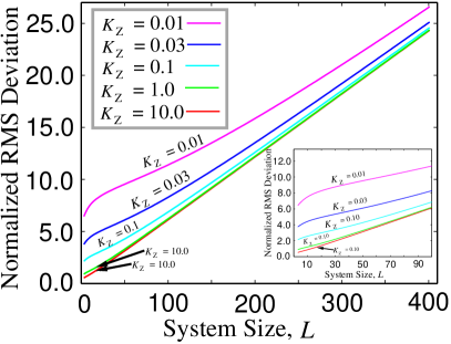
Figure 19: Normalized mean square displacements for $K_{z}$ = 0.01, 0.03, 0.1, 1.0, and 10.0 for the dual-layer square lattice with an extended coupling scheme, where $K_{z}$ is in units of the intralayer coupling $K$. The inset is a closer view of the RMS curves.

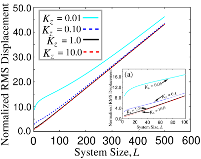
Figure 20: Normalized mean square displacements for $K_{z}$ = 0.01, 0.1, 1.0, and 10.0 for the dual-layer tetrahedral lattice where $K_{z}$ is in units of the triangular lattice intra-layer coupling $K$. The inset is a closer view of the RMS curves.

Figure 21: Normalized Eigenvalue Density of States for the dual-layer cubic system with with nearest and next-nearest neighbor interactions (a) and for the dual-layer locally stiff lattice based on a tetrahedral lattice geometry (b) for system size $L=5001$.

While adjusting the interaction between the layers to enhance the resistance to local transverse perturbations has little effect on the mean square fluctuations for large values of $L$, the eigenvalue density of states evolves as the interplanar to intraplanar coupling ratio $\kappa_{z}=K_{z}/K$ is modified. Density of states profiles for $\kappa_{z}$ values ranging from $\kappa_{z}=0.1$ to $\kappa_{z}=3.0$ are shown for the dual-layer square system with and extended coupling pattern in Fig. 22 and for the tetrahedral counterpart in Fig. 23.

Density of states profiles are shown for strong ($\kappa_{z}=3.0$) and moderate ($\kappa_{z}=1.0$) values of the the coupling ratio in insets (a) and (b) of Fig. 22 and Fig. 23, and there is little change in the DOS curve in the low eigenvalue regime. On the other had, as $\kappa_{z}$ decreases further and the interplanar coupling begins to fall below parity with that in the plane, the eigenvalue density of states profiles begin to change more drastically, as may be seen in panels (b) and (c) of Fig. 22 for the dual-layer square system and Fig. 23 for the dual-layer tetrahedrally based geometry; the distribution in both cases rapidly grows narrower with decreasing $\kappa_{z}$. Although the two lattice geometries are very distinct, similar (and likely generic to locally rigid dual-layer lattices) trends may be seen in the DOS profiles in the regime of low eigenvalues as $\kappa_{z}$ is reduced.

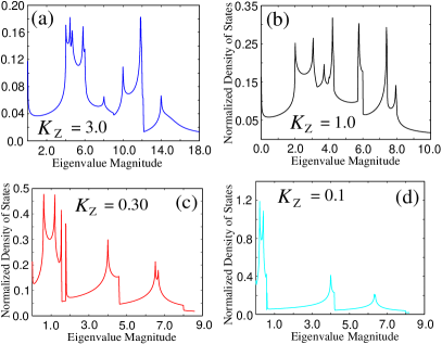
Figure 22: Normalized density of states profiles for $K_{z}$ = 3.0, 1.0, 0.3, and 0.1 for the dual-layer square lattice with an extended coupling scheme where $K_{z}$ is in units of the triangular lattice intra-layer coupling $K$.

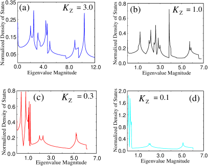
Figure 23: Normalized density of states profiles for $K_{z}$ = 3.0, 1.0, 0.3, and 0.1 for the dual-layer tetrahedral lattice where $K_{z}$ is in units of the triangular lattice intra-layer coupling $K$.

VI Coupling to a Substrate

We incorporate an attractive interaction with a flat substrate by including an additional harmonic potential acting on the lower members of the tetrahedral and square extended coupling dual-layer systems. We take the attraction to depend only on the atomic shift $\delta^{\mathrm{I}z}_{ij}$ above the planar system, and the additional term hence has the form $\frac{K_{s}}{2}\left(\delta_{ij}^{Iz}\right)^{2}$

Figure 24 shows the effect of the substrate coupling on $\delta_{\mathrm{RMS}}$ in the case of the dual-layer square system with an extended coupling scheme. The graph, which shows mean square deviation curves for a wide range of $K_{s}$ values, indicates the capacity of even a very mild substrate coupling to suppress thermally induced undulations in the dual-layer sheet. Similarly, for the tetrahedrally based dual-layer lattice geometry, an attractive interaction with a substrate considerably reduces fluctuations transverse to the lattice planes, preventing a rapid divergence of $\delta_{\mathrm{RMS}}$. The mean square deviation curves are shown in Figure 25.

We also examine the effect of an attractive substrate coupling on the density of states profiles, and results are displayed in Fig. 26 for a range of substrate coupling constants $K_{s}$. With increasing $K_{s}$, a salient trend is the opening of a separation between the sharp cusp and the zero eigenvalue mark on the abscissa. The migration of the maximum formerly at the zero eigenvalue point to a peak at a larger eigenvalue is associated with a sharp reduction of the mean square fluctuations about equilibrium, and the lattice is better able to withstand transverse fluctuations.

The presence of a flat substrate plays a very important role in dictating the overall structure and amplitude of ripples in the dual-layer geometries we report on here. This result is in accord with recent experiments on graphene sheets deposited on cleaved mica substrates Lui (2009), where the careful preparation of flat substrates significantly dampens the ripple amplitude, whereas much larger undulations are seen with sheets attached to substrates with poorer control over the flatness.

To determine which length scales are associated with the strongest contributions to the thermally averaged mean square deviations about equilibrium, we have prepared histograms showing the relative contribution to $\delta_{\mathrm{RMS}}$ versus inverse wave-vector magnitude, with the latter providing a length scale. Apart from a significant diminution in the height of thermally excited undulations in the dual-layered sheets, we also find a considerable reduction in their typical wavelength. In figure 27, for the dual-layer tetrahedral lattice in the absence of a substrate couplings, the dominant contribution to $\delta_{\mathrm{RMS}}$ comes from large length scales comparable to the scale of the lattice. However the picture changes with the activation of a finite substrate coupling as may be seen in the inset with the peak height at the minimal wave-number decreasing with increasing $K_{s}$. Moreover, as may be seen in Figure 28, introducing even a weak anchoring to the foundation below immediately creates a strong peak in the short wavelength regime, skewing the size of thermally induced ripples toward smaller length scales.

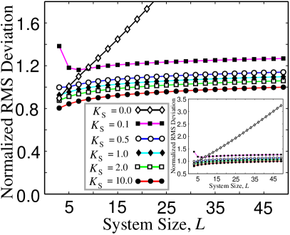
Figure 24: For the dual-layer square lattice in the extended scheme, the main figure and the inset are graphs of mean square fluctuations versus system size $L$ for a range of substrate couplings $K_{s}$, with $K_{s}$ given in units of the inter-planar and intra-planar coupling constant (both equal to $K$). The symbol legend on the main plot also pertains to the inset

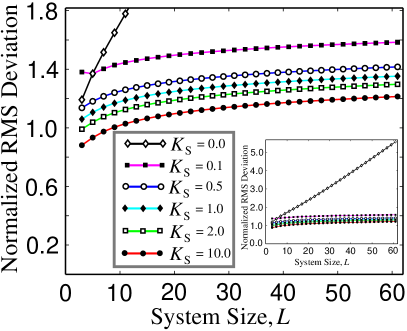
Figure 25: For the dual-layer tetrahedral lattice, the main figure and the inset are graphs of mean square fluctuations versus system size $L$ for a range of substrate couplings $K_{s}$, with $K_{s}$ given in units of the inter-planar and intra-planar coupling constant (both equal to $K$). The symbol legend on the main plot also pertains to the inset

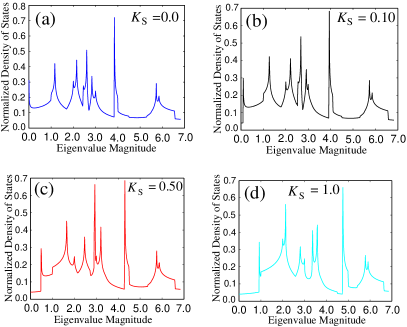
Figure 26: Normalized Density of States for the Dual layer system for various substrate coupling strengths $K_{s}$. Panels (a), (b), (c), and (d) show the density of states for $K_{s}$ equal to $0.0$, $0.1$, $0.5$, and $1.0$ respectively.

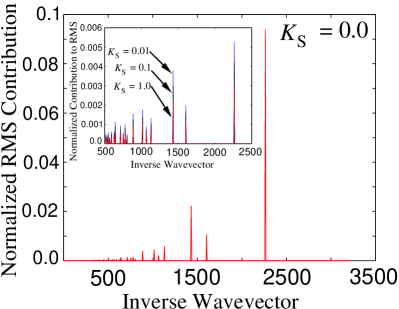
Figure 27: Normalized Eigenvalue Density of States for the dual-layer triangular system with system size $L=5001$.

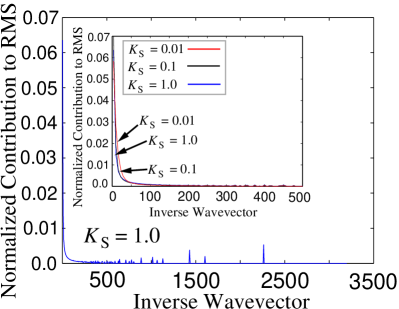
Figure 28: Normalized Eigenvalue Density of States for the dual-layer triangular system with system size $L=5001$.

In conclusion, we have examined thermally induced fluctuations about equilibrium in two and three dimensional crystalline solids with a local bonding scheme. While long-range crystalline order may exist in three dimensional crystal lattices, some geometries (e.g. the simple cubic lattice) are not rigid when only nearest-neighbor couplings are taken into account, and an extended coupling scheme is needed to prevent the divergence of mean square fluctuations with increasing system size $L$.

In two dimensional lattices, we find RMS fluctuations to increase at a very slow (logarithmic) rate when motion is confined to the lattice plane. On the other hand, when transverse motion is permitted, thermal fluctuations are very effective in bringing about significant vertical displacements of particles which contribute to rapidly growing deviations from equilibrium, and $\delta_{\mathrm{RMS}}$ ultimately diverges at a linear rate in $L$. The asymptotically linear divergence in the mean square deviations from equilibrium is insensitive to the strength of the interlayer coupling; $\delta_{\mathrm{RMS}}$ values appear to converge and eventually show identical behavior with increasing system size whether the coupling $K_{z}$ established between the layers to provide local stiffness is quite weak or very strong relative to the bonding $K$ between atoms in the same layer.

Introducing a coupling $K_{s}$ to a flat substrate very effectively hinders transverse fluctuations in two dimensional crystal lattices, even in the coupling is very weak, and reflects the importance of a substrate in shaping the characteristics of ripples set up by thermal fluctuations by inhibiting transverse deviations. An attractive coupling to a fixed substrate also reduces the typical lateral length scale or wavelength of thermally excited undulations in lattices bound to a substrate. These tendencies are consistent with recent experimental observations that control over the flatness of the underlying surface is directly related to the amplitude and length scale of thermally induced ripples.

References

Lindemann (1910)
F. Lindemann
Z. Phys. 11,
609 (1910).
Chaikin (2000)
P. M. Chaikin and
T. C. Lubensky,
Principles of Condensed Matter Physics,
(2000).
Metropolis (1953)
N. Metropolis,
A. W. Rosenbluth,
M. N. Rosenbluth,
A. H. Teller,
E. Teller
The Journal of Chemical Physics 20,
6,1087
(1953).
Lui (2009)
C. H. Lui,
Li Liu,
K. F. Mak,
G. W. Flynn,
T. F. Heinz,
Nature 462,
3392009
(2009).