The dependence of the EIT wave velocity on the magnetic field strength

Abstract

“EIT waves” are a wavelike phenomenon propagating in the corona, which were initially observed in the extreme ultraviolet (EUV) wavelength by the EUV Imaging Telescope (EIT). Their nature is still elusive, with the debate between fast-mode wave model and non-wave model. In order to distinguish between these models, we investigate the relation between the EIT wave velocity and the local magnetic field in the corona. It is found that the two parameters show significant negative correlation in most of the EIT wave fronts, i.e., EIT wave propagates more slowly in the regions of stronger magnetic field. Such a result poses a big challenge to the fast-mode wave model, which would predict a strong positive correlation between the two parameters. However, it is demonstrated that such a result can be explained by the fieldline stretching model, i.e., that “EIT waves” are apparently-propagating brightenings, which are generated by successive stretching of closed magnetic field lines pushed by the erupting flux rope during coronal mass ejections (CMEs).

1 Introduction

S-Introduction EIT waves were discovered by the EUV Imaging Telescope (EIT) [Delaboudinière et al. (1995)] aboard the Solar and Heliospheric Observatory (SOHO) initially in the 195 Å channel [Moses et al. (1997), Thompson et al. (1999)]. They are transient wavelike disturbances that propagate almost over the solar disk and are followed by expanding dimmings (Thompson et al., 1998; 1999). Later, they were also identified in other channels like 171 Å, 284 Å, and 304 Å Wills-Davey and Thompson (1999); Zhukov and Auchère (2004); Long et al. (2008). They originate in around a flare site and propagate outward, avoiding strong magnetic features and neutral lines and stopping near coronal holes Thompson et al. (1999) or near the magnetic separatrix between active regions Delannée and Aulanier (1999). The intriguing phenomenon provoked a lot of controversies on the driving source and its nature (e.g., Del00; chen08). It becomes now widely accepted that EIT waves are physically associated with CMEs, rather than solar flares Biesecker et al. (2002); Cliver et al. (2005); Chen (2006). Especially, chen09a and dai10 found that EIT wave fronts are cospatial with CME frontal loops.

The debate on the nature of EIT waves has been continuing for more than 10 years. EIT waves were initially explained as the counterparts of chromospheric Moreton waves Thompson et al. (1999). Moreton waves are propagating fronts visible mainly in the H$\alpha$ line wings, traveling with a velocity of 500-2000 km s^-1 Moreton and Ramsey (1960). They were successfully explained to be due to coronal fast-mode waves sweeping the chromosphere (e.g., Uchida). Following this line of thought, wang00 and wu01 numerically compared the propagation of fast-mode waves with the EIT wave observations, and claimed that the trajectory of the fast-mode wave front matches the EIT wave very well. The cospatiality of a sharp front in the EIT image with the H$\alpha$ Moreton wave front in the 1997 September 24 event reinforced such a conjecture Thompson et al. (2000). However, there is dispute about the relation between this sharp EIT wave front and the ensuing diffuse EIT wave fronts. Some authors, e.g., warm05, propose that the sharp front evolves to the diffuse fronts, whereas others, e.g., chen05, suggest that they are of different origin, with the sharp front being the real coronal Moreton wave, and the ensuing diffuse fronts being the so-called EIT wave in the general sense. In their model, the sharp front moved out of the solar disk and was not visible in the ensuing EIT images since the cadence of SOHO/EIT, $\sim 15$ min, is too long.

The fast-mode model for EIT waves was first questioned by Del99, who proposed that EIT waves should be related to magnetic reconfiguration. Based on MHD numerical simulations, chen02 proposed that EIT waves are apparently moving brightenings which are generated by the successive stretching of the closed field lines, being pushed by the erupting flux rope. The theory can explain the following observational features: (1) EIT wave velocity is typically 3 times slower than fast-mode wave velocity; (2) A substantial outflow is present in the dimming region, and absent in the EIT wave front Harra and Sterling (2003); (3) EIT wave velocity is uncorrelated with type II radio bursts velocity Klassen et al. (2000). The model is also consistent with the statistical studies which show that EIT waves are more closely associate with CME than solar flares Biesecker et al. (2002); Chen (2006). Besides, some authors proposed alternative models in terms of slow-mode waves Wills-Davey et al. (2007); Wang, Shen, and Lin (2009) or successive reconnection Attrill et al. (2007).

According to the fast-wave model, it is expected to see a strong positive correlation between EIT wave velocity and the local fast-mode wave velocity or the local magnetic field strength. However, in the fieldline stretching model of Chen et al. (2002; 2005), the EIT wave velocity is determined by both magnetic field strength and magnetic configuration Chen (2009b), e.g., a strongly stretched configuration as in a quadrupolar field leads to a small EIT wave velocity. Therefore, it would not see a significant positive correlation between EIT wave velocity and the local fast-mode wave velocity or the field strength. In particular, chen09b theoretically showed that as the EIT wave propagates outward just across the boundary of the source active region, the fast-mode wave velocity decreases with the distance, whereas the EIT wave velocity increases. Therefore, it is easy to distinguish the fast-wave model and the fieldline stretching model by studying the correlation between EIT wave velocities and the local magnetic field strength, which is the aim of this paper. Observations and the data analysis are described in Section 2, the results are presented in Section 3, and discussions are given in Section 4.

2 Observations and Data Analysis

S-general The two EIT wave events studied in this paper took place on 2007 May 19 and 2007 December 7. Both were located near the solar disk center in the field of view of the Extreme Ultra Violet Imager (EUVI) Howard et al. (2008) on board the Solar Terrestrial Relations Observatory Ahead (STEREO A) satellite, which allows a precise measurement of the EIT wave velocity.

There are four channels in STEREO/EUVI observations, i.e., 171 Å (the formation temperature $T$ $\sim$ 1 MK), 195 Å ($T$ $\sim$ 1.5 MK), 284 Å ($T$ $\sim$ 2 MK), and 304 Å. It is noted that the 304 Å channel has a coronal contribution from the Si XI line ($T$ $\sim$ 1.6 MK), in addition to the chromospheric line He II ($T$ $\sim$ 80000 K) Brosius et al. (1996); Long et al. (2008). Although EIT waves are more evident in 195 Å than 171 Å Wills-Davey and Thompson (1999), we use the 171 Å images to derive the EIT wave propagation velocities since the time cadence ($\sim$ 2.5 min) is much shorter than that of the 195 Å channel ($\sim$ 10 min).

In order to derive the strength of the coronal magnetic field, we use the potential field extrapolated from the synoptic magnetogram of Michelson Doppler Imager (MDI) telescope Scherrer et al. (1995) on board the SOHO satellite with the potential field source surface (PFSS) technique Schrijver and Derosa (2003). Since EIT wave fronts are significantly bright in the low corona (e.g., cohen09), the magnetic field is taken at the height of 0.06$R_{\odot}$ in the extrapolated potential field.

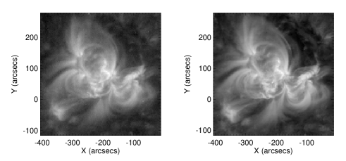
Figure 1.: The image of SOHO/EIT (left) and the corrected image of STEREO/EUVI (right) at 15:24:00 UT on 2007 May 19 in the bandpass 171 Å. The correlation coefficient of the two images is 0.96.fig:519

Since the STEREO/EUVI and SOHO/MDI observe the Sun at different times and directions, an important step is to coalign these two data sets. For that purpose, both data sets are coaligned with SOHO/EIT images, since EUVI and EIT use the same emission lines, while MDI and EIT are both aboard the SOHO satellite. First, we derotate and remap the images of EUVI to that of EIT. As an example, the two panels of Figure fig:519 display the corrected 171 Å images from SOHO/EIT (left) and STEREO/EUVI (right) at 15:24:00 UT on 2007 May 18 . The correlation coefficient of the two images is 0.96. After being remapped to the Earth view, running difference images of STEREO/EUVI are taken to show the propagation of EIT waves. As an example, Figure diffq depicts the evolution of the EIT wave event on 2007 May 19. Second, the distribution of the radial component of the magnetic field ($B_{r}$) at the height of 0.06 $R_{\odot}$ is taken from the extrapolated coronal field, and is derotated and remapped to the same time as the EUVI images. Figure pfssq shows the corresponding $B_{r}$ distribution for the two EIT wave events. Note that $B_{r}$ is the main component of the magnetic field outside active regions.

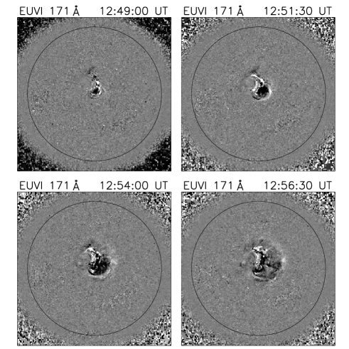
Figure 2.: The base difference images of the EIT wave event at 4 times from 12:49:00 UT to 12:56:30 UT on 2007 May 19 observed by STEREO/EUVI showing the wave propagation and the dimming regions on the solar disk. The black circles mark the solar limb.diffq

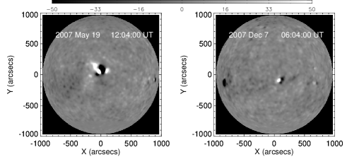
Figure 3.: The corrected full disk distributions of the radial component of magnetic field ($B_{r}$) at the height of $0.06R_{\odot}$ for the two EIT events, which are extrapolated from the MDI magnetogram on the solar surface.pfssq

3 Results

S-features From the running difference images as shown in Figure diffq, we can manually trace the location of the EIT wave front at each time, which is illustrated in Figure 4 as solid lines. As the EIT wave front appears diffuse with time and the magnetic field become weak far away from the active region, we measure the EIT wave propagation close to the active region only. The left panel displays the propagation of the EIT waves at 6 times from 12:46:30 UT to 12:59:00 UT for the 2007 May 19 event, and the right panel displays the propagation of the EIT waves at 6 times from 04:28:30 UT to 04:41:00 UT for the 2007 December 7 event. Note that only the evident portion of each EIT wave front is traced, so that the first event is traced mainly in the west hemisphere, whereas the second event in the east hemisphere.

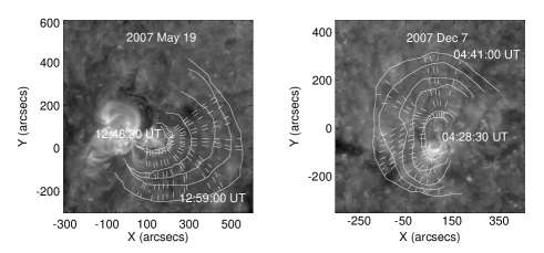
Figure 4.: Huygens plotting of the EIT wave front propagation in the 2007 May 19 event (left) and the 2007 December 7 event (right) in the bandpass 171 Å. The solid lines correspond to the wave fronts at different times, while the dashed lines show the propagating trajectories.gt

In order to derive the propagation velocity, we select 20 starting points along the first visible EIT wave front, and then track their trajectories with the Huygens plotting technique as done in wills99 and zhu09. The trajectories are displayed as dashed lines in Figure gt. The velocity is obtained by the 3-point central difference scheme. Therefore, for each trajectory, velocities at 4 times can be obtained. Error in wave front position is estimated to be $\pm$2 pixels, following zhu09. The local magnetic field at each position is determined by averaging the surrounding $3\times 3$ pixels in the extrapolated coronal field at the height of 0.06$R_{\odot}$ above the solar surface.

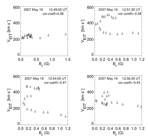
Figure 5.: The relation between EIT wave velocity and magnetic field strength for the 2007 May 19 event. The four panels correspond to 12:49:00 UT, 12:51:30 UT, 12:54:00 UT, 12:56:30 UT, respectively.vcor519

The scatter plot of the EIT wave velocity ($v_{\rm EIT}$) vs. the radial component of the magnetic field ($B_{r}$) for the 2007 May 19 event is displayed in Figure vcor519, where 4 panels correspond to wave fronts at 12:49:00 UT, 12:51:30 UT, 12:54:00 UT, and 12:56:30 UT. It is seen that, only at 12:49:00 UT, a very weak positive correlation exists between $v_{\rm EIT}$ and $B_{r}$ (upper left panel), where $v_{\rm EIT}$ increases slightly as $B_{r}$ increases by more than 10 times. In the ensuing times, however, $v_{\rm EIT}$ and $B_{r}$ present a negative correlation, where EIT waves tend to move more slowly at the site with a stronger magnetic field.

The scatter plot of $v_{\rm EIT}$ vs. $B_{r}$ for the 2007 December 7 event is displayed in Figure vcor127, where 4 panels correspond to the EIT wave fronts at 04:28:30 UT, 04:31:00 UT, 04:33:30 UT, and 04:36:00 UT, respectively. All these panels reveal that $v_{\rm EIT}$ is negatively correlated to $B_{r}$, with the correlation coefficient being smaller than -0.7 at 3 times.

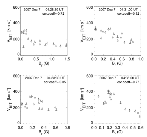
Figure 6.: The relation between the EIT wave velocity and the magnetic field strength for the 2007 December 7 event. The four panels correspond to 04:28:30 UT, 04:31:00 UT, 04:33:30 UT, 04:36:00 UT, respectively.vcor127

4 Discussions

S-Conclusion

“EIT waves” are often explained in terms of fast-mode magnetoacoustic waves in the corona (e.g., wang00; wu01; vrs02; war04; gre08; pom08; gop09; pat09). However, the wave model cannot explain the following features of “EIT waves” (see wils07; chen08, for details): (1) the “EIT wave” velocity is significantly smaller than those of Moreton waves. The latter are well established to be due to fast-mode waves in the corona; (2) the “EIT wave” velocities have no correlation with those of type II radio bursts Klassen et al. (2000); (3) the “EIT wave” fronts may stop when they meet with magnetic separatrices Delannée and Aulanier (1999); (4) the EIT wave velocity may be below 100 km s^-1 (e.g., Dav08), which is even smaller than the sound speed in the corona. Moreover, the rotation of EIT wave fronts reported by pod05 was found to be linked to the filament rotation, implying that EIT waves might not be fast-mode waves Attrill et al. (2007). Note that it may be argued that the lack of correlation between the velocities of EIT waves and type II radio bursts is due to that the former is located at the leg, while the latter is at the top of the same fast-mode wave. However, the velocities of Moreton waves and type II radio bursts do show linear correlation Pinter (1977), although Moreton wave is also located at the leg of the type II radio burst-related shock wave.

In order to distinguish whether EIT waves are fast-mode waves or not, we investigated the relation between the EIT wave velocity and the local magnetic field with the high-cadence observations from STEREO/EUVI. With the Huygens plotting technique, EIT wave velocity distribution along each front at 4 times from two EIT wave events was derived, it is found that except at one moment when the EIT wave velocity ($v_{\rm EIT}$) is slightly positively correlated with the local magnetic field ($B_{r}$), $v_{\rm EIT}$ at all other moments is negatively correlated with $B_{r}$, and at some moments, the negative correlation is rather significant. In order to examine the validity of the result, we also calculated the relation between $v_{\rm EIT}$ and $B_{r}$, with $B_{r}$ being taken at heights like 0.3$R_{\odot}$ and 0.1$R_{\odot}$, it is found that the result does not change. Such a result poses a big challenge to the fast-mode wave model for EIT waves, since the model would predict a strong positive correlation between $v_{\rm EIT}$ and $B_{r}$.

It would be then interesting to check whether the significant negative correlation between $v_{\rm EIT}$ and $B_{r}$ can be explained by the fieldline stretching model proposed by Chen et al. (2002; 2005). The fieldline stretching model is illustrated in Figure cartoon: as the flux rope is ejected upward, all the overlying field lines will be pushed to stretch up, and for each fieldline, the stretching starts from the top part. That is to say, the perturbation propagates from point A to C with the fast-mode wave speed, by which the EIT wave front reaches point C. Note that the fast-mode wave speed along the magnetic field line is equal to the Alfvén speed $v_{A}$. Then the perturbation propagates from point A to B and then to D with the local fast-mode wave speed $v_{f}=\sqrt{v_{A}^{2}+v_{s}^{2}}$ (here $v_{s}$ is the sound speed), by which a second front reaches point D. The apparent velocity of the EIT wave is the distance CD divided by the time difference of the perturbation transfer, i.e.,

$$v_{\rm EIT}=CD/\Delta t,\ilabel{equ}$$ (1)

where $\Delta t=\int_{A}^{B}1/v_{f}ds+\int_{B}^{D}1/v_{A}ds-\int_{A}^{C}1/v_{A}ds$. According to this model, we can calculate the EIT wave velocity profile for any magnetic configuration.

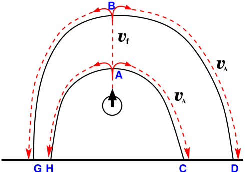
Figure 7.: Sketch of the fieldline stretching model for EIT waves proposed by Chen et al. (2002, 2005), where solid lines are the magnetic field, and dashed lines indicate how the magnetic fieldline stretching is transferred with the local fast-mode wave speed, i.e., the Alfvén speed $v_{A}$ along the field line and $v_{f}=\sqrt{v_{A}^{2}+v_{s}^{2}}$ perpendicular to the field line, where $v_{s}$ is the sound speed.cartoon

In order to get an asymmetric magnetic configuration, we put an oblique magnetic dipole below the solar surface, with a line current (along the $z$-direction) at $x=-2.4$ and $y=-5.5$ , and another line current (along the negative $z$-direction) at $x=-2.6$ and $y=-5.7$. The magnetic field is plotted in the left panel of Figure num, with the typical magnetic field being $\sim 3.3$ G. From the figure we can see that the magnetic field left to the magnetic neutral line is stronger than that to the right. For simplicity, we assume a uniform and isothermal plasma with the plasma number density of $10^{8}$ cm^-3 and temperature of $10^{6}$ MK. The resulting typical Alfvén speed is $v_{A0}$=900 km s^-1. The corresponding EIT wave velocity profile, which is calculated with Equation (equ), is depicted in the right panel of Figure num, where the wave velocity is in unit of $v_{A0}$. It is seen that the EIT wave velocity profile is complicated. Within $|x|\leq$ 2, the EIT wave velocity ($v_{\rm EIT}$) is higher on the left side, whereas as $|x|$ is larger than 2, $v_{\rm EIT}$ becomes higher on the right side. This means that for the magnetic field in the left panel of Figure num, $v_{\rm EIT}$ and $B_{r}$ are correlated positively near the neutral line and negatively further out. Such a result is qualitatively consistent with the observed features presented in Section 3.

By comparing the top two panels in either Figure vcor519 or Figure vcor127, it can also be seen that both events analyzed in this paper show that EIT wave velocity increases as the front propagates outward near the boundary of the source active region. This confirms the result presented in Dav08. chen09b claimed that this feature poses another big challenge for the fast-mode wave model for EIT waves, which implies a deceleration of EIT wave velocity away from the active region since the fast-mode wave speed is much larger near the active region than in the quiet region. chen09b also demonstrated that the acceleration can be well accounted for in the fieldline stretching model. The reason is quite straightforward: according to their model Chen et al. (2002, 2005), as illustrated in Figure cartoon, if the magnetic configuration is strongly stretched, i.e., the distance between points B and C is larger, the apparent EIT wave velocity derived by Equation (equ) would be smaller. The boundary of active regions does present such a kind of stretched magnetic configuration, as demonstrated in chen09b. vero08 also analyzed the 2007 May 19 event, however, they claimed that the EIT wave velocity decreases with the distance from the source active region as expected from the fast-mode wave model. The discrepancy between their results and ours, as well as in Dav08, is probably due to that they did not show the EIT wave propagation before 12:52:00 UT, when the EIT wave velocity was increasing.

Figure 8.: Left: an asymmetric magnetic configuration corresponding to an oblique magnetic dipole below the solar surface; Right: the corresponding EIT wave velocity distribution along the horizontal distance. The velocity is in unit of 900 km s^-1.num

Note that we focused our study on the EIT wave propagation near the source active region, where the significant variation of the EIT wave velocity happens. In the quiet region far from the source active region, the EIT wave velocity becomes relatively stable Ma et al. (2009). With a suitable choice of the coronal density model, it would be easier to reproduce the EIT wave propagation in the large scale as done by wang00 and wu01, especially when there were only $\sim 3$ snapshots of EIT wave propagation in the SOHO era. However, it is hard to imagine that the negative correlation between EIT wave velocity and the local magnetic field strength near the boundary of the source active region can be reproduced in the fast-mode wave framework.

To summarize, we analyzed the relation between EIT wave velocity ($v_{\rm EIT}$) and the local magnetic field ($B_{r}$) in two events observed by STEREO/EUVI with a high cadence. It is found that $v_{\rm EIT}$ and $B_{r}$ are negatively correlated in most of the fronts, except along one front where $v_{\rm EIT}$ and $B_{r}$ show a weak positive correlation. It is further revealed that such features, which pose a big challenge for the fast-wave model for EIT waves, can be well explained by the fieldline stretching model proposed by Chen et al. (2002; 2005).

Acknowledgements

The research is supported by the Chinese foundations 2006CB806302 and NSFC (10403003, 10933003, and 10673004). We thank the referee for constructive comments that helped to improve the paper and M. L. Derosa for the help on the use of PFSS routine. The SECCHI data used here were produced by an international consortium of USA, UK, Germany, Belgium, and France. SOHO is a project of international cooperation between ESA and NASA.

References

- Attrill et al. (2007) Attrill, G.D.R., Harra, L.K., van Driel-Gesztelyi, L., and Démoulin, P.: 2007, Astrophys. J. 656, L101.
- Biesecker et al. (2002) Biesecker, D.A., Myers, D.C., Thompson, B.J., Hammer, D.M., and Vourlidas, A.: 2002, Astrophys. J. 569, 1009.
- Brosius et al. (1996) Brosius, J.W., Davila, J.M., Thomas, R.J., and Monsignori-Fossi, B.C.: 1996, Astrophysical Journal Supplement Series 106, 143.
- Chen (2006) Chen, P.F.: 2006, Astrophys. J. 641, L153.
- Chen (2008) Chen, P.F.: 2008, J.Astrophys.Astron. 29, 179.
- Chen (2009a) Chen, P.F.: 2009a, Astrophys. J. 698, L112.
- Chen (2009b) Chen, P.F.: 2009b, Sci. in China (G) 52, 1785.
- Chen et al. (2005) Chen, P.F., Fang, C., and Shibata, K.: 2005, Astrophys. J. 622, 1202.
- Chen et al. (2002) Chen, P.F., Wu, S.T., Shibata, K., and Fang, C.: 2002, Astrophys. J. 572, L99.
- Cliver et al. (2005) Cliver, E.W., Laurenza, M., Storini, M., and Thompson, B.J.: 2005, Astrophys. J. 631, 604.
- Cohen et al. (2009) Cohen, O., Attrill, G.D.R., Manchester, W.B., and Wills-Davey, M.J.: 2009, Astrophys. J. 705, 587.
- Dai et al. (2010) Dai, Y., Auchère, F., Vial, J.-C., Tang, Y.H., and Zong, W.G.: 2010, Astrophys. J. 708, 913.
- Delaboudinière et al. (1995) Delaboudinière, J.-P., Artzner, G.E., Brunaud, J., et al.: 1995, Solar Phys. 162, 291.
- Delannée (2000) Delannée, C.: 2000, Astrophys. J. 545, 512.
- Delannée and Aulanier (1999) Delannée, C., and Aulanier, G.: 1999, Solar Phys. 190, 107.
- Gopalswamy et al. (2009) Gopalswamy, N., Yashiro, S., Temmer, M., et al.: 2009, Astrophys. J. 691, L123.
- Grechnev et al. (2008) Grechnev, V.V., Uralov, A.M., Slemzin, V.A., Chertok, I.M., Kuzmenko, I.V., and Shibasaki, K.: 2008, Solar Phys. 253, 263.
- Harra and Sterling (2003) Harra, L.K., and Sterling, A.C.: 2003, Astrophys. J. 587, 429.
- Howard et al. (2008) Howard, R.A., Moses, J.D., Vourlidas, A., et al.: 2008, Space Science Reviews 136, 67.
- Klassen et al. (2000) Klassen, A., Aurass, H., Mann, G., and Thompson, B.J.: 2000, Astron. Astroph. 141, 357.
- Long et al. (2008) Long, M.D., Peter, T.G., R.T., Mcateer, J., and Bloomfield, D.S.: 2008, Astrophys. J. 680, L81.
- Ma et al. (2009) Ma, S., Wills-Davey, M.J., Lin, J., et al.: 2009, Astrophys. J. 707, 503.
- Moreton and Ramsey (1960) Moreton, G.E., and Ramsey, H.E.: 1960, Publications of the Astronomical Society of the Pacific 72, 357.
- Moses et al. (1997) Moses, D., Clette, F., Delaboudinière, J.-P., et al.: 1997, Solar Phys. 175, 571.
- Patsourakos et al. (2009) Patsourakos, S., Vourlidas, A., Wang, Y.M., Stenborg, G., and Thernisien, A.: 2009, Solar Phys. 259, 49.
- Pinter (1977) Pinter, S. 1977, Spec. Rep. AFGL-SR-209, Hanscom Air Force Base, 35.
- Podladchikova and Berghmans (2005) Podladchikova, O. and Berghmans, D.: 2005, Solar Phys. 228, 265.
- Pomoell et al. (2008) Pomoell, J., Vainio, R., and Kissmann, R.: 2008, Solar Phys. 253, 249.
- Scherrer et al. (1995) Scherrer, P.H., Bogart, R.S., Bush, R.I., et al.: 1995, Solar Phys. 162, 129.
- Schrijver and Derosa (2003) Schrijver, C.J., and Derosa, M.L.: 2003, Solar Phys. 212, 615.
- Thompson et al. (1999) Thompson, B.J., Gurman, J.B., Neupert, W.M., et al.: 1999, Astrophys. J. 517, L151.
- Thompson et al. (1998) Thompson, B.J., Plunkett, S.P., Gurman, J.B., Newmark, J.S., St. Cyr, O.C., and Michels, D.J.: 1998, Geophys. Res. Lett. 25, 2465.
- Thompson et al. (2000) Thompson, B.J., Reynolds, B., Aurass, H., et al.: 2000, Solar Phys. 193, 161.
- (34) Uchida, Y.: 1968, Solar Phys. 39, 431.
- Veronig, Temmer, and Vršnak (2008) Veronig, A.M., Temmer, M., and Vršnak, B.: 2008, Astrophys. J. 681, L113.
- Vršnak et al. (2002) Vršnak, B., Warmuth, A., Brajša, R., and Hanslmeier, A.: 2002, Astron. Astroph. 394, 299.
- Wang (2000) Wang, Y.M.: 2000, Astrophys. J. 543, L89.
- Wang, Shen, and Lin (2009) Wang, H., Shen, C., and Lin, J.: 2009, Astrophys. J. 700, 1716.
- Warmuth, Mann, and Aurass (2005) Warmuth, A., Mann, G., and Aurass, H.: 2005, Astrophys. J. 626, L121.
- Warmuth et al. (2004) Warmuth, A., Vršnak, B., Magdalenić, J., Hanslmeier, A., and Otruba, W.: 2004, Astron. Astroph. 418, 1101.
- Wills-Davey et al. (2007) Wills-Davey, M.J., DeForest, C.E., and Stenflo, J.: 2007, Astrophys. J. 644, 556.
- Wills-Davey and Thompson (1999) Wills-Davey, M.J., and Thompson, B.J.: 1999, Solar Phys. 190, 467.
- Wu et al. (2001) Wu, S.T., Zheng, H., Wang, S., Thompson, B.J., et al.: 2001, Journal of Geophysical Research 106, 25089.
- Zhukov and Auchère (2004) Zhukov, A.N., and Auchère, F.: 2004 Astron. Astroph. 427, 705.
- Zhukov et al. (2009) Zhukov, A.N., Rodriguez, L., and de Patoul, J.: 2009, Solar Phys. 259, 73.