Čerenkov radio pulses from electromagnetic showers in the time-domain

Abstract

The electric field of the Čerenkov radio pulse produced by a single charged particle track in a dielectric medium is derived from first principles. An algorithm is developed to obtain the pulse in the time domain for numerical calculations. The algorithm is implemented in a Monte Carlo simulation of electromagnetic showers in dense media (specifically designed for coherent radio emission applications) as might be induced by interactions of ultra-high energy neutrinos. The coherent Čerenkov radio emission produced by such showers is obtained simultaneously both in the time and frequency domains. A consistency check performed by Fourier-transforming the pulse in time and comparing it to the frequency spectrum obtained directly in the simulations yields, as expected, fully consistent results. The reversal of the time structure inside the Čerenkov cone and the signs of the corresponding pulses are addressed in detail. The results, besides testing algorithms used for reference calculations in the frequency domain, shed new light into the properties of the radio pulse in the time domain. The shape of the pulse in the time domain is directly related to the depth development of the excess charge in the shower and its width to the observation angle with respect to the Čerenkov direction. This information can be of great practical importance for interpreting actual data.

I Introduction

It was nearly 50 years ago that Askaryan proposed to detect high energy particles through the coherent pulse they emit as they interact in a dense medium Askaryan62 . As secondary electrons, positrons and gamma rays are produced they develop electromagnetic showers in the medium which acquire an excess negative charge, which Askaryan estimated to be of order $10\%$ of the total number of electrons and positrons. This is so in spite of the interactions being completely charge symmetric, because matter in the medium only contains electrons. Møller, Bhabha and Compton scattering of matter electrons, accelerate them into the shower while electron-positron annihilation and Bhabha scattering decelerate the shower positrons thus also contributing to the excess charge, a mechanism referred to as the Askaryan effect. A more accurate calculation of the Askaryan effect indicated that the excess charge is actually $\sim 25\%$ of the total number of electrons and positrons ZHS92 . Such an excess charge develops a coherent electromagnetic pulse as it travels through a non absorptive dielectric medium. The coherent part of the pulse is mainly due to the wavelength components which are large compared to the shower width. The energy radiated in the coherent pulse scales with the square of the excess charge and hence with the square of the shower energy. Such scaling naturally makes the detection of coherent radio pulses an attractive and promising technique for the detection of ultra high energy particles, such as cosmic rays.

Radio detection of air showers was extensively studied in the 60’s and 70’s allan71 . The drive to detect high energy neutrinos in the late 80’s turned back the attention onto radio pulses produced by them in dense media such as natural ice frichter96 or the regolith beneath the Moon’s surface zheleznykh . The first full simulations of the Askaryan effect and the coherent pulses created in dense media were obtained in the early 90’s ZHS92 ; ZHS91 , which allowed more quantitative calculations and experimental programs were soon after started to search for neutrinos with arrays of antennas at Antarctica RICE98 or with radio telescopes from Earth Parkes96 . The Askaryan effect was measured for the first time firing photon bunches into sand at SLAC in 2000 Saltzberg_SLAC_sand - and later in other dielectric media including ice Gorham_SLAC_salt ; Miocinovic_SLAC_sand ; Gorham_SLAC_ice - and since then the field has received an enormous boost, strengthening previous initiatives using antennas buried in ice  RICE03 ; RICElimits and radiotelescopes Parkes07 , and developing new ones such as a balloon flown antenna array ANITAlite ; ANITA_2009_limits ; ANITAlong , new radiotelescope searches GLUElimits ; Kalyazin ; NuMoon ; LUNASKA ; RESUN and new radio measurements of air showers ARENA08 .

The first calculation of the radio emission from electromagnetic showers used a specifically designed Monte Carlo simulation code - the ZHS code - to calculate coherent radio pulses in ice ZHS91 ; ZHS92 . The code has been extended to include the LPM effect alz97 , to calculate in an approximate manner hadronic showers alz98 and neutrino-induced showers alvz99 , to treat other dielectric media alvz06 , and to perform an optimal statistical thinning that allows the simulation of pulses from ultrahigh energy showers aljpz09 , and remains as a reference in the field. This code was designed to calculate the Fourier components of the electric field in the frequency domain. Alternative simulations using other codes such as GEANT3 almvz03 ; razzaque04 , GEANT4 almvz03 ; razzaque04 ; McKay_radio and the AIRES+TIERRAS TIERRAS ; alctz10 code, have yielded results compatible to within $\sim 5\%$. Semi-analytical calculations have also been performed buniy02 . All of these use the same technique to calculate the radio pulse in the frequency domain, but to our knowledge no full calculation exists in the time domain yet.

All experimental arrangements measure the electric field as a function of time, and full understanding of the properties of the pulse as a function of time is thus also very important. Although the conversion from the frequency to the time domain is in principle straightforward and the algorithm in ZHS computes all required information to obtain it, there have been a number of doubts concerning the unconventional choice of Fourier transform as used in the code ZHS92 , as well as the sign, phase and causality properties of the pulse buniy02 , that have complicated the analysis and interpretation of data.

In this article we develop a formalism to calculate the pulse directly in the time domain. We simultaneously calculate the pulse of the same electromagnetic shower in both the time and frequency domains. An exhaustive comparison yields fully compatible results, makes patent the relative advantages of each approach, and sheds new light into the properties of the radio pulse in the time domain which can be related to those of the shower and can be of great practical importance in interpreting actual data. Some of these properties are discussed in more detail suggesting possible applications.

Although the method developed in ZHS92 , and extended here to the time-domain, has been obtained in the framework of Čerenkov radiation, it derives directly from Maxwell’s equations and addresses classical radiation from charges in a pretty general fashion. Simple extensions of this work can be used for instance to calculate transition radiaton as particles cross dielectric media interfaces or to calculate the complete radiation patterns from charges moving in magnetic fields including Čerenkov radiation, as has been known for long to be important for ultra high energy air showers.

This paper is structured as follows. In Section II we rederive the expression for the electric field in both the time and frequency domain in a form that can be easily used for practical applications and make the connection to the expression derived in the original ZHS paper ZHS92 . We also discuss some simple current density models and relate them to the results of a full electromagnetic shower simulation. In Section III we perform a consistency check by Fourier-transforming the pulse in time and comparing it to the frequency spectrum obtained in the simulations. The summary and outlook constitute the last section.

II Theory and Monte Carlo implementation

II.1 Theory

We start from Maxwell’s equations for linear, isotropic, homogeneous and non dispersive media. In the International System of units:

$$\mathbf{\nabla}\cdot\mathbf{E} =\frac{\rho}{\epsilon} \mathbf{\nabla}\times\mathbf{E} =-\frac{\partial\mathbf{B}}{\partial t}$$ (1)

$$\mathbf{\nabla}\cdot\mathbf{B} =0 \mathbf{\nabla}\times\mathbf{B} =\mu\mathbf{J}+\mu\epsilon\frac{\partial\mathbf{E}}{\partial t}$$ (2)

where $\rho$ is the charge density of the source, $\epsilon=\epsilon_{\rm r}\epsilon_{0}$ and $\mu=\mu_{\rm r}\mu_{0}$ are the total permittivity and permeability expressed in terms of the relative ($\mu_{\rm r}$ and $\epsilon_{\rm r}$) and free space ($\mu_{0}$ and $\epsilon_{0}$) permittivities and permeabilities. All effects of induced currents and electric polarization are automatically accounted for by the displacement field $\mathbf{D}=\epsilon\mathbf{E}$ proportional to the electric field, $\mathbf{E}$ and the magnetic field strength $\mathbf{H}=(\mu)^{-1}\mathbf{B}$, proportional to the magnetic field, $\mathbf{B}$.

We recall the formal solution introducing the vector and scalar potentials ($\mathbf{A}$ and $\phi$):

$$\mathbf{B} =\mathbf{\nabla}\times\mathbf{A}$$ (3)

$$\mathbf{E} =-\frac{\partial\mathbf{A}}{\partial t}-\mathbf{\nabla}\phi$$ (4)

that naturally satisfy $\mathbf{\nabla}\cdot\mathbf{B}=0$, and the equation involving the $\mathbf{\nabla}\times\mathbf{E}$ term. Choosing the transverse gauge, in which $\mathbf{\nabla}\cdot\mathbf{A}=0$, the two remaining equations imply:

$$\nabla^{2}\phi =-\frac{\rho}{\epsilon}$$ (5)

$$\nabla^{2}\mathbf{A}-\mu\epsilon\frac{\partial^{2}\mathbf{A}}{\partial^{2}t} =-\mu\mathbf{J}_{\perp}$$ (6)

where $\mathbf{J}_{\perp}$ is the transverse current, a divergenceless component of the current density, which in the limit of observation at large distances from the source can be shown to correspond to the projection of the current density perpendicular to the direction of observation (of unit vector $\hat{\mathbf{u}}$), i.e., ${\mathbf{J}}_{\perp}=-\hat{\mathbf{u}}\times(\hat{\mathbf{u}}\times\mathbf{J})$.

Both equations can be formally solved using Green’s functions:

$$\phi =\frac{1}{4\pi\epsilon}\int\frac{\rho(\mathbf{x^{\prime}},t^{\prime})}{|\mathbf{x}-\mathbf{x^{\prime}}|}d^{3}\mathbf{x^{\prime}}$$ (7)

$$\mathbf{A} =\frac{\mu}{4\pi}\int\frac{\mathbf{J}_{\perp}(\mathbf{x^{\prime}},t^{\prime})}{|\mathbf{x}-\mathbf{x^{\prime}}|}\delta\left(\sqrt{\mu\epsilon}|\mathbf{x}-\mathbf{x^{\prime}}|-(t-t^{\prime})\right)d^{3}\mathbf{x^{\prime}}dt^{\prime}$$ (8)

The first is the familiar solution from electrostatics for the potential produced at the position $\mathbf{x}$ by a source with charge density $\rho(\mathbf{x^{\prime}},t^{\prime})$. The second is the solution of the wave equation with wave velocity $(\epsilon_{0}\mu_{0}\epsilon_{\rm r}\mu_{\rm r})^{-{1\over 2}}$ smaller than the velocity of light in vacuum, $c=(\epsilon_{0}\mu_{0})^{-{1\over 2}}$, by a factor $n=(\epsilon_{\rm r}\mu_{\rm r})^{-{1\over 2}}$, the index of refraction. The Green’s function for the wave equation involves a delta function that gives the familiar retarded time, $t^{\prime}$, earlier than the observing time $t$. To evaluate the field at time $t$ at a given position $\mathbf{x}$, the current is to be evaluated at a time retarded by the time taken by light to reach observation point from point $\mathbf{x^{\prime}}$, i.e. $|\mathbf{x}-\mathbf{x^{\prime}}|n/c$.

II.2 Radiation from charges traveling in straight lines

We consider the shower as a superposition of finite particle tracks of constant velocity. Each track is completely defined by two limiting times $t_{1}$ and $t_{2}$, its velocity $\mathbf{v}$ and the position vector of an arbitrary point of the track, $\mathbf{x_{0}}$, which we have chosen to correspond to the time $t=0$. The transverse current density entering in Eq. (8) for a point charge moving with constant velocity, $\mathbf{v}$, between the two end points simply reads :

$$\mathbf{J}_{\perp}(\mathbf{x^{\prime}},t^{\prime})=e\mathbf{v}_{\perp}\delta^{3}\left(\mathbf{x^{\prime}}-\mathbf{x_{0}}-\mathbf{v}t^{\prime}\right)\left[\Theta(t^{\prime}-t_{1})-\Theta(t^{\prime}-t_{2})\right]$$ (9)

where $-e$ is the charge of an electron, $\mathbf{v}_{\perp}$ is the projection of the velocity onto a plane perpendicular to the direction of observation (recall that we consider large distances so that this direction is uniquely defined), and $\Theta(x)$ is the Heaviside step function.

We can now substitute the transverse current into Eq.(8), integrate the three dimensional delta function substituting $\mathbf{x^{\prime}}$ for $\mathbf{x_{0}}+\mathbf{v}t^{\prime}$ and approximate the distance between $\mathbf{x}$ and $\mathbf{x^{\prime}}$ by $|\mathbf{x}-\mathbf{x_{0}}-\mathbf{v}t^{\prime}|\simeq R-\mathbf{v}\cdot\hat{\mathbf{u}}t^{\prime}$, where we define $R=|\mathbf{x}-\mathbf{x_{0}}|$. In the limit of large distances of observation the denominator $|\mathbf{x}-\mathbf{x^{\prime}}|$ can be simply approximated by $R$. However, we must use the above approximation in the argument of the retarding delta function to account for interference effects. This corresponds to the Fraunhofer approximation, in which the path difference between light pulses emitted at points $\mathbf{x_{0}}$ and $\mathbf{x^{\prime}}=\mathbf{x_{0}}+\mathbf{v}t^{\prime}$ is simply the distance between them projected onto the direction of observation. As a result the delta function reads $\delta\left(t^{\prime}(1-n\beta\cos\theta)-\left(t-{nR\over c}\right)\right)$, with $\mathbf{v}=\mbox{\boldmath{$\beta$}}c$, which can be cast into:

$${1\over|1-n\beta\cos\theta|}\delta\left(t^{\prime}-{t-{nR\over c}\over 1-n\beta\cos\theta}\right)$$ (10)

We note that the recurring factor $(1-n\beta\cos\theta)$, with $\theta$ the angle between $\mathbf{v}$ and $\hat{\mathbf{u}}$, gives zero for the Čerenkov angle $\theta_{C}$. Moreover the factor changes sign from positive to negative as the observation angle changes from being larger to smaller than the Čerenkov angle. Now we can perform the integration in $t^{\prime}$ in Eq. (8) which simply implies replacing $t^{\prime}$ in the step functions by ${t-{nR\over c}\over 1-n\beta\cos\theta}$. We now make use of the fact that:

$$\Theta(ax)=\begin{cases}\Theta(x)~{}\text{ if $a>0$},\\ 1-\Theta(x)~{}\text{ if $a<0$}\end{cases}$$ (11)

In this equation we can take $a=(1-n\beta\cos\theta)^{-1}$ and $x=t-nR/c-(1-n\beta\cos\theta)t_{1,2}$ which allows us to rewrite Eq.(8) as:

$$\begin{split}&\mathbf{A}={\mu e\over 4\pi R}\mathbf{v}_{\perp}\\ &{\Theta(t-{nR\over c}-(1-n\beta\cos\theta)t_{1})-\Theta(t-{nR\over c}-(1-n\beta\cos\theta)t_{2})\over(1-n\beta\cos\theta)}\end{split}$$ (12)

Note that the modulus in the denominator of Eq.(10) is removed because of an effective $\mbox{sgn}(1-n\beta\cos\theta)$ that appears when changing the argument in the two step functions (according to Eq. (11)). This expression is easy to implement in a shower simulation by splitting particle tracks in portions that can be approximated by uniform motion.

As $\theta$ approaches the Čerenkov angle $\theta_{C}$ the numerator and denominator of Eq.(12) approach zero. To obtain a formal limit for the Čerenkov angle we multiply and divide by $\delta t$ to obtain:

$$\begin{split}&R\mathbf{A}(t,\theta)=\frac{e\mu_{r}}{4\pi\epsilon_{0}c^{2}}{\mathbf{v}}_{\perp}\delta t\\ &\frac{\Theta\left(t-{nR\over c}-(1-n\beta\cos\theta)t_{1}\right)-\Theta\left(t-{nR\over c}-(1-n\beta\cos\theta)t_{2}\right)}{(1-n\beta\cos\theta)\delta t}\end{split}$$ (13)

The limit $\theta\to\theta_{C}$ is equivalent to $(1-n\beta\cos\theta)\delta t\to 0$ which can be shown to give the first derivative of the step function, the function $\delta(t)$. The limit is then:

$$R\mathbf{A}(t,\theta_{C})=\left[\frac{e\mu_{r}}{4\pi\epsilon_{0}c^{2}}\right]\delta\left(t-{nR\over c}\right){\mathbf{v}}_{\perp}\delta t$$ (14)

We note that the vector potential in this limit is simply proportional (and parallel) to ${\mathbf{v}}_{\perp}\delta t$, i.e. to the projection of the displacement vector onto a plane perpendicular to the observation direction. This expression can also be implemented in a shower simulation provided a suitable approximation is made for the delta function.

The expression for the electric field is given by Eq. (4) and only the term with the time derivative of the vector potential gives contribution to the radiation term so that:

$$\begin{split}&R\mathbf{E}(t,\theta)=-\frac{e\mu_{r}}{4\pi\epsilon_{0}c^{2}}{\mathbf{v}}_{\perp}\\ &\frac{\delta\left(t-{nR\over c}-(1-n\beta\cos\theta)t_{1}\right)-\delta\left(t-{nR\over c}-(1-n\beta\cos\theta)t_{2}\right)}{(1-n\beta\cos\theta)}\end{split}$$ (15)

Figure 1: Schematic representation of the radiation fields in the time domain induced by a single particle with positive charge $e>0$ traveling at constant velocity $\beta$ between times $t_{1}$ and $t_{2}$. Top panel vector potential (see Eq.(12)). Bottom panel electric field (see Eq.(15)). See also text for more details.

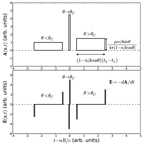
The radiation field due to a single particle track with $e>0$ is similar to the schematic diagram shown in Fig. 1. Such a particle produces radiation when the track starts or ends. The two pulses “as seen” by the observer (placed at angle $\theta$ w.r.t. the particle track) are separated by a time interval associated to the difference in propagation time $(1-n\beta\cos\theta)\delta t$.

Let us first consider an angle exceeding the Čerenkov angle so that $(1-n\beta\cos\theta)$ is positive. The electric field of the first pulse corresponds to the start point of the track ($t_{1}$) and it is anti-parallel to $\mathbf{v}_{\perp}$ according to Eq.(15), while it is parallel for the second pulse which corresponds to the end point ($t_{2}$). The sign of the electric field pulse is opposite to the sign of the particle acceleration in both cases. The zero in the shown arrival time is arbitrary and corresponds to $t={nR/c}$, i.e. it is a reference time associated to the arrival of a signal from the reference position $\mathbf{x_{0}}$. The two pulses associated with the track take place later than this reference time.

As the angle decreases and becomes smaller than the Čerenkov angle, the situation is reversed: The first pulse corresponds to the end point of the track ($t_{2}$), while the second corresponds to the start point ($t_{1}$). Moreover not only is the arrival of the pulses as seen by the observer inverted, but both take place before the reference time. This apparent acausal behavior is due to the fact that the particle travels at a speed greater than that of light in the medium. Although the terms responsible for the first and second pulses are interchanged, and there is a sign change associated with this interchange, it is compensated by the denominator of Eq.(4) that also reverses its sign. As a result there is no change in the sign of the electric field of the first and second pulses as the Čerenkov angle is crossed, and the double peak structure at any given time has the same qualitative behavior as the observation angle changes. This seems physically sound since there can be no discontinuity of the electric field across the Čerenkov cone boundary.

For observation at the Čerenkov angle both signals arrive simultaneously. In this limiting case the electric field can be formally obtained taking minus the derivative of the delta function given by Eq.(14). This again corresponds to a double pulse first antiparallel and then parallel to $\mathbf{v}_{\perp}$.

II.3 Equations in the Frequency Domain

The expression for the electric field in the frequency domain used in the ZHS simulation code (Eq.(12) in ZHS92 ) reads:

$$\mathbf{E}(\omega,\mathbf{x})={e\mu_{\rm r}\over 2\pi\epsilon_{0}{\rm c}^{2}}~{}i\omega~{}{{\rm e}^{ikR}\over R}~{}{\rm e}^{i(\omega-\mathbf{k}\cdot\mathbf{v}){\rm t}_{1}}~{}\mathbf{v}_{\perp}~{}\left[{{\rm e}^{i(\omega-\mathbf{k}\cdot\mathbf{v})\delta{\rm t}}-1\over i(\omega-\mathbf{k}\cdot\mathbf{v})}\right]$$ (16)

We recall that this equation has been obtained with the following convention for the Fourier transform of the electric field:

$$\tilde{f}(\omega)=2\int_{-\infty}^{\infty}{f}(t)~{}e^{i\omega t}dt$$ (17)

where the factor 2 corresponds to an unusual convention (this factor is usually either 1 or $(2\pi)^{-{1\over 2}}$). Applying this Fourier transform definition to Eq.(15) giving the electric field in the time domain we obtain:

$$\begin{split}\mathbf{E}(\omega,\mathbf{x})=&-{e\mu_{\rm r}\over 2\pi\epsilon_{0}{\rm c}^{2}}~{}{1\over R}~{}\mathbf{v}_{\perp}\\ &{{\rm e}^{i\omega\left[nR/c+(1-n\beta\cos\theta)\right]{\rm t}_{1}}-{\rm e}^{i\omega\left[nR/c+(1-n\beta\cos\theta)\right]{\rm t}_{2}}\over(1-n\beta\cos\theta)}\end{split}$$ (18)

which can be easily rearranged to give exactly Eq. (16) noting that $k={n\omega\over c}$. Moreover if we apply the Fourier transform to Eq.(14) which applies to the limit $\theta\rightarrow\theta_{C}$ we get:

$$R\mathbf{A}(\omega,\mathbf{x})={e\mu_{\rm r}\over 2\pi\epsilon_{0}{\rm c}^{2}}~{}\mathbf{v}_{\perp}\delta t~{}{\rm e}^{i(\omega{\rm t_{1}}-\mathbf{k}\mathbf{r}_{1})}~{}{\rm e}^{ikR}$$ (19)

The electric field is obtained taking minus the time derivative which in Fourier space is just a factor $i\omega$, giving again the same result as Eq.(13) in ZHS92 for the electric field in the frequency domain at the Čerenkov angle.

These calculations show the consistency of Eq.(15) obtained in the time domain with Eq.(16) which gives the field in the frequency domain: They are simply Fourier transforms of each other as expected.

II.4 Pulses for Simple Charge Distributions

Before performing a Monte Carlo simulation of electromagnetic showers, it is interesting to extend the calculations to simple models for the shower. These models allow us to obtain relations between the shape of the pulse in the time domain and the time and spatial distribution of the charge.

A simple yet interesting model consists of a charge $Q(z^{\prime})$ that rises and falls along the shower direction $z^{\prime}$ and spreads laterally in $x^{\prime}$ and $y^{\prime}$. Assuming cylindrical symmetry we can write the current associated to this charge distribution as:

$$\mathbf{J}(\mathbf{x^{\prime}},t^{\prime})=\mathbf{v}f(z^{\prime},\mathbf{r^{\prime}})Q(z^{\prime})\delta(z^{\prime}-vt^{\prime})$$ (20)

Here $\mathbf{r^{\prime}}$ is a two dimensional vector in the $(x^{\prime},y^{\prime})$ plane transverse to $z^{\prime}$, and the function $f(z^{\prime},\mathbf{r^{\prime}})$ gives the charge distribution in such a plane as a function of shower depth, with normalization chosen so that $Q$ indeed gives the excess charge:

$$\int d^{2}\mathbf{r}f(z^{\prime},\mathbf{r})=\int_{0}^{2\pi}d\phi^{\prime}\int^{\infty}_{0}f(z^{\prime},r^{\prime},\phi^{\prime})=1$$ (21)

with $\phi^{\prime}$ the azimuthal angle in cylindrical coordinates.

The simplest case is that of a line current along the $z^{\prime}$ direction without lateral extension in which $f(x^{\prime},y^{\prime})$ is replaced by the two dimensional delta function $\delta(x^{\prime})\delta(y^{\prime})$. This approximation was also discussed in alvz99 in the frequency domain, where it was referred to as the one-dimensional approximation. When such line current is substituted into Eq.(8) and integrated in $x^{\prime}$, $y^{\prime}$ and $t^{\prime}$ making the Fraunhofer approximation, a relatively simple expression is obtained that relates the vector potential in the time domain to the excess charge $Q(z^{\prime})$:

$$\begin{split}R\mathbf{A}=&\frac{\mu}{4\pi}\mathbf{v}_{\perp}\\ &\int_{-\infty}^{\infty}dz^{\prime}Q(z^{\prime})\delta\left[z^{\prime}(1-n\beta\cos\theta)-v\left(t-{nR\over c}\right)\right]\end{split}$$ (22)

The delta function relates the depth in the shower development $z^{\prime}$ to the observation time $t$ through a linear function:

$$z^{\prime}=\zeta(t)=\beta{ct-nR\over 1-n\beta\cos\theta}$$ (23)

As the observation angle approaches the Čerenkov angle, the time interval corresponding to the depth spanned by the shower, i.e. the pulse width, becomes smaller. We thus recover a familiar result already discussed in ZHS92 although in the frequency domain.

Performing the integration in Eq.(22) yields,

$$R\mathbf{A}=\frac{\mu c\beta}{4\pi}\frac{\mathbf{v}_{\perp}}{|1-n\beta\cos\theta|}Q(\zeta(t))$$ (24)

where the delta function in Eq.(22) introduces a factor $|1-n\beta\cos\theta|^{-1}$.

The electric field is obtained taking minus the derivative of the vector potential with respect to time:

$$R\mathbf{E}=-\frac{\mu c\beta}{4\pi}{\mathbf{v}_{\perp}\over(1-n\beta\cos\theta)|1-n\beta\cos\theta|}\left.{dQ(\zeta)\over d\zeta}\right|_{\zeta=\beta{ct-nR\over 1-n\beta\cos\theta}}$$ (25)

The factor $(1-n\beta\cos\theta)^{-1}$ arises from applying the chain rule to the derivative of $Q[\zeta(t)]$. As a result the pulse in the time domain can be regarded as the derivative of the development of the charge excess along the shower, scaled with the Čherenkov factors $(1-n\beta\cos\theta)^{-1}$ and $|1-n\beta\cos\theta|^{-1}$, and converted from depth into time through Eq.(23), i.e., the pulse is firstly positive and then negative with respect to $\mathbf{v}_{\perp}$ since in a real shower $Q(z^{\prime})$ corresponds to an excess of negative charge.

A number of interesting results can be directly read off Eq.(25). If the development curve for the excess charge $Q(z^{\prime})$ is not symmetric, as happens in real showers, the asymmetry in its derivative is directly reflected into an asymmetry between the negative and positive parts of the pulse. Also it is interesting to note that when the angle of observation is below the Čerenkov angle, the pulse shape is inverted in time because the early part of the pulse corresponds to the end of the shower while the beginning of the shower corresponds to the end part of the pulse, as explained above. Still, the polarity of the first and second pulses remains the same because, although the slopes before and after shower maximum change sign, there is an extra sign change induced by the factor $(1-n\beta\cos\theta)^{-1}$. This is in complete analogy to what was discussed for a single track.

In the case of observation in the Čerenkov direction, the $z^{\prime}$ dependence of the delta function in Eq.(22) disappears and the delta function can be factored away from the integral, to give a pulse of amplitude directly proportional to the integrated excess track length of the shower. The delta function term is due to all parts of the line current being observed simultaneously at the Čerenkov angle. These are two familiar results already emphasized in ZHS92 .

The simulation has shown that the model with the absence of a lateral distribution breaks down at $|\theta-\theta_{C}|\lesssim 2.5^{\circ}$. This result is consistent with that found in alvz99 where the one dimensional model was studied in the frequency domain.

It is instructive to extend the line current model to a more realistic three dimensional current $f(z^{\prime},r)$ with cylindrical symmetry and current given in Eq.(20). In that case the expression for the vector potential with two delta functions can be integrated in $t^{\prime}$ and $\phi^{\prime}$ and the resulting expression involves a double integral over cylindrical coordinate $r^{\prime}$ and the shower depth $z^{\prime}$:

$$\begin{split}&R\mathbf{A}=\mathbf{v_{\perp}}\frac{\mu}{2\pi}\int_{0}^{\infty}r^{\prime}dr^{\prime}\int_{-\infty}^{\infty}dz^{\prime}f(z^{\prime},r^{\prime})Q(z^{\prime})\\ &\frac{\Theta(n\beta r^{\prime}\sin\theta-|z^{\prime}(1-n\beta\cos\theta)-(vt-n\beta R)|)}{\sqrt{\left[n\beta r^{\prime}\sin\theta\right]^{2}-\left[z^{\prime}\left(1-n\beta\cos\theta\right)-\left(vt-n\beta R\right)\right]^{2}}}\end{split}$$ (26)

This expression, despite being more cumbersome than Eq.(22), if solved analytically for realistic lateral distribution functions, could give insight into useful parametrizations of the pulse in the time domain. In any case it can be used for numerical simulations.

In the Čerenkov limit Eq.(26) becomes

$$\begin{split}&R\mathbf{A}=\frac{\mu}{2\pi}\frac{\mathbf{v_{\perp}}}{n\beta\sin\theta_{C}}\int_{-\infty}^{\infty}dz^{\prime}Q(z^{\prime})\\ &\int_{\frac{|vt-n\beta R|}{n\beta\sin\theta_{C}}}^{\infty}\frac{r^{\prime}dr^{\prime}f(z^{\prime},r^{\prime})}{\sqrt{r^{\prime 2}-\left[\frac{vt-n\beta R}{n\beta\sin\theta_{C}}\right]^{2}}}\end{split}$$ (27)

This equation shows that the non-zero width of the electromagnetic pulse at the Čerenkov angle is the result of the lateral distribution of the shower. Although the integral is rather complicated to evaluate for realistic lateral shower profiles, it can be shown that for distributions of the form $f(r^{\prime})=(r^{\prime})^{-n}$ for integers $n>2$ the electric field $\mathbf{E}\propto\mathbf{v}_{\perp}\mbox{sgn}(t-nR/c)|vt-n\beta R|^{-n}$, which is a fast bi-polar pulse of non-zero width.

This model still has some limitations. Note that Eq.(27) predicts a pulse that is symmetric in time while simulations have shown that the pulse at the Cerenkov angle is asymmetric. This is due in part to the radial distribution of velocities of the shower which is not included in the model. The development of a current density vector model that can accurately produce the features of Čerenkov radiation is work in progress.

II.5 Implementation in the ZHS Monte Carlo

The ZHS Monte Carlo ZHS92 allows the simulation of electromagnetic showers and their associated coherent radio emission up to EeV energies aljpz09 . Originally developed in ice ZHS91 , it has been extended so that electromagnetic showers in other dielectric homogeneous media can be simulated alvz06 ; aljpz09 . The code accounts for bremsstrahlung, pair production, and the four interactions responsible for the development of the excess charge, namely Møller, Bhabha, Compton scattering and electron-positron annihilation. In addition multiple elastic scattering (according to Molière’s theory) and continuous ionization losses are also implemented. The electron/positron tracks between each interaction are split into subtracks so that no subtrack exceeds a maximum depth fixed at 0.1 radiation lengths. For low energy particles these subdivisions are actually reduced to ensure that no subtrack is comparable to the particle range, and they become the step used to evaluate ionization losses and multiple elastic scattering. Convergence of results as the step is reduced has been carefully checked alvz00 .

In order to account for interference effects between the radiation emitted due to the particles responsible for the excess negative charge, the ZHS code was designed to follow all electrons and positrons down to 100 keV kinetic energy threshold, as well as to carefully account for time, by considering deviations with respect to a plane front moving at the speed of light injected in phase with the primary particle. In addition to the delays associated to the propagation geometry, those due to particles travelling at velocities smaller than the velocity of light are accounted for assuming the energy loss is uniform across the step. An approximate account is also made of the time delay associated to the multiple elastic scattering processes along the step.

As a result the tracks of all charged particles in a shower are divided into multiple subtracks which are assumed to be straight and to have constant velocity. The positions of the end points of these subtracks as well as the corresponding times are readily available by design, and they can be used to compute the frequency components of the electric field making extensive use of Eq.(16), taking into account the relative phase shift between different tracks because of their different starting point positions and time delays.

In this work we have extended the Monte Carlo to also calculate the pulse in the time domain. A routine has been developed to account for contributions of each of these particle subtracks to the vector potential, making extensive use of Eq.(12). Each subtrack contributes a unit “rectangle” to the vector potential, which varies in height, “duration” and sign - see Fig. 1, depending on the velocity, the relative orientation of the track with respect to the direction of observation and the charge of the particle. When the observation direction is very close to the Čerenkov angle the delta function in Eq.(14) is replaced by a rectangle corresponding to a nascent delta function Kelly . If the sampling time bin width is set to $\Delta T$ then a natural choice of nascent delta function is given by

$$\eta_{\Delta T}(t)=\left\{\begin{array}[]{l l}\frac{1}{\Delta T},&\quad-\frac{\Delta T}{2}<t\leq\frac{\Delta T}{2}\\ 0,&\quad\mbox{otherwise}\\ \end{array}\right.$$ (28)

In this case the base of the rectangle is fixed by the intrinsic “time resolution” $\Delta T$ of the simulation and the pulse height depends on $\Delta T$. In practice, the time domain radio signal can be reconstructed with an antenna receiver system and digital sampling electronics. The time resolution of a single waveform is determined by the digital sampling bin width and the high frequency cutoff of the receiver system.

Once the vector potential induced by each subtrack is defined, the contribution of all charged subtracks in the shower is obtained and the vector potential is derived with respect to time to obtain the electric field in the time domain.

In the next Section we show several examples of the results of this procedure.

III Results

In Fig. 2 we show the electric field as a function of arrival time of the signal obtained with the ZHS code in a single 1 PeV electron-induced shower in ice for different observation angles. The zero in the shown arrival time is measured with respect to the arrival time of a pulse emitted as the primary particle initiating the shower is injected in the medium.

Figure 2: Electric field as a function of time as obtained in ZHS simulations of a single 1 PeV electron-induced shower in ice for different observation angles. Top panel: Observation at the Čerenkov angle, bottom panel: observation at $\theta_{C}-5^{\circ}$ (long green dashes) and at $\theta_{C}+5^{\circ}$ (short blue dashes). In the bottom panel the red solid histograms represent the electric field obtained applying Eq.(25) to the simulated excess negative charge $Q(z)$.

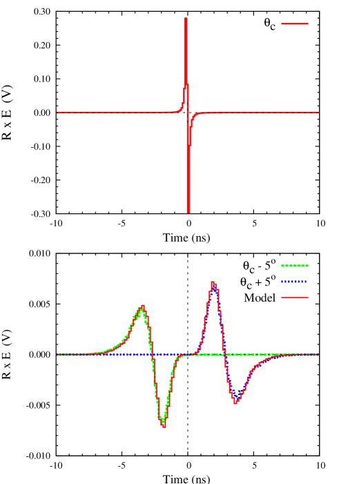
The electric field is parallel to the projection of the velocity onto a plane perpendicular to the direction of the observation at early times and anti-parallel later on. This is expected after the discussion in Section II.2 of the electric field emitted by a single positively charged particle, with the important difference that in a shower the electric field is produced by an excess of negative charge and the polarity of the field is reversed with respect to that shown in Fig. 1. Also as in the case of a single track there is no change in the polarity of the pulse when observing inside ($\theta<\theta_{c}$) or outside ($\theta>\theta_{c}$) the Čerenkov cone ($\theta_{c}$). The pulse always starts being positive (parallel to $\mathbf{v}_{\perp}$) and ends being negative (antiparallel to $\mathbf{v}_{\perp}$) regardless of the observation angle. This feature can be used as a discriminator against background events for neutrino searches. It can be also clearly seen that the pulse is broader in time away from the Čerenkov cone than close to it with an apparent duration proportional to $\Delta z|1-n\beta\cos\theta|/c$ with $\Delta z$ being the spread along the shower axis of the excess charge (see Eq.(23)). For observation at the Čerenkov angle the apparent duration of the pulse is not zero, despite the fact that the Čerenkov factor $|1-n\beta\cos\theta_{c}|\rightarrow 0$, because the shower spreads out also in the lateral dimensions ($x$ and $y$ directions). Also due to our definition of $t=0$ and to the presence of the Čerenkov factor in the $\delta-$functions in Eq.(15), the pulse occurs at $t>0$ outside the Čerenkov cone and at $t<0$ inside it.

Figure 3: Top panel: Longitudinal development of the excess negative charge as obtained in ZHS simulations of 1 PeV (long green dashes) and 100 PeV (short blue dashes) electron-induced showers in ice. Bottom panel: Electric field as a function of time generated in the showers shown in the top panel (dashed histograms), for observation angle $\theta_{C}+10^{\circ}$. The solid histograms represent the electric field obtained applying Eq.(25) to the simulated excess charge $Q(z)$ shown in the top panel.

According to the simple model developed in Section II.4 the field away from the Čerenkov angle is proportional to the derivative of the excess charge distribution $Q(z)$ with respect to $t$ - Eq.(25) - or equivalently the derivative with respect to $z$ since there is a linear relation between $t$ and $z$ - Eq.(23). The ZHS code also gives the longitudinal profile of the excess charge and we have applied Eq.(25) to the simulated $Q(z)$, and compared to the electric field obtained directly in the Monte Carlo. This is also shown in Fig. 2. The agreement between the electric field obtained directly in the Monte Carlo simulation (dashed histograms) and what is predicted by Eq.(25) (solid histograms) is remarkable. The electric field follows the variation of the excess charge in $z$ or equivalently in $t$. This explains why for a fixed observation angle the pulse changes sign from early to late times (for a typical shower $Q(z)$ grows relatively fast, reaches a maximum, and then decreases more slowly with depth), and why it is asymmetric with respect to the time axis ($Q(z)$ is not a symmetric function around its maximum). Also when the direction of observation is inside the Čerenkov cone, the observer sees the derivative of the beginning of the excess charge distribution first and the corresponding derivative of the end of $Q(z)$ at later times, while the opposite is true for observations outside the Čerenkov cone. As a consequence the pulse at $\theta<\theta_{c}$ looks like an antisymmetric copy with respect to $t=0$ of the pulse at $\theta>\theta_{c}$, as can be clearly seen in Fig. 2. An accurate reconstruction of the time domain electric field could in principle determine on which side of the Cerenkov cone the event was observed. On the other hand the shape of the pulse can be conversely used to infer the depth development of the shower.

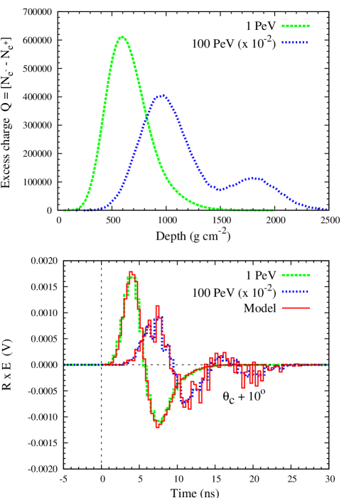
Eq.(25) stresses the fact that the features of the excess charge distribution are “mapped” in the time structure of the pulse. In particular it is well known that electromagnetic showers with energies above the energy scale at which the LPM effect LPM starts to be effective ($\sim$ PeV in ice Stanev_LPM ), are “stretched” in the longitudinal dimension and often show peaks in their profile RalstonLPM ; Konishi ; alz97 ; klein . These two features should translate into the duration in time also of the pulse and into its time structure that should also exhibit multiple peaks. This is shown in Fig. 3 in which due to the LPM effect the longitudinal profile of a 100 PeV electron-induced shower exhibits two peaks which appear as 2 positive and 2 negative peaks in the time structure of the pulse. For comparison a 1 PeV electron-induced shower not affected by the LPM effect and its corresponding electric field are also shown. The linear relation between the time domain structure of an electric field and the shower profile suggests that the longitudinal profile of the shower could be reconstructed from an observation off the Čerenkov angle.

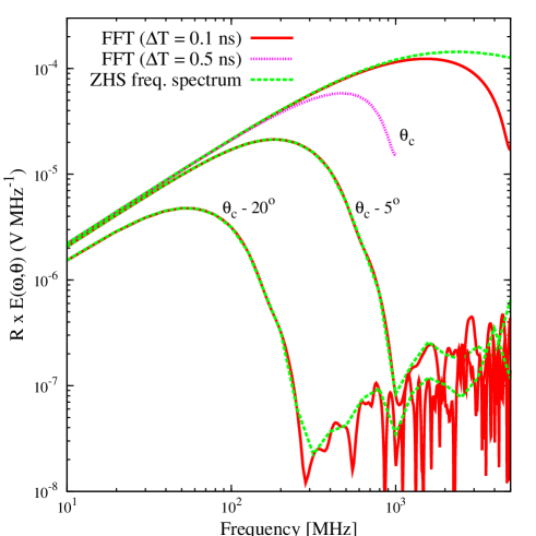
The extended ZHS code is able to calculate both the electric field as a function of time and its Fourier transform from first principles. Moreover, the two calculations can be made simultaneously for the same shower. Both calculations can be easily compared by performing the Fourier transform of the pulse calculated in the time domain, following the convention in Eq.(17). This provides a further check of the two methods, as well as a test of accuracy in the numerical procedures involved in the calculation of the radio emission in both domains. An example is shown in Fig. 4, where the electric field as a function of frequency as obtained in ZHS simulations of a single 1 PeV electron-induced shower is plotted along with the (Fast) Fourier Transform (FFT) of the electric field in the time domain obtained in simultaneous ZHS simulations of the same shower. The agreement between both spectra is very good for frequencies below $\omega_{\Delta T}\sim 2\pi/\Delta T$ with $\Delta T$ an arbitrary time resolution needed for the ZHS simulations in the time domain. We do not expect to be able to reproduce the frequency spectrum at frequencies above $\omega_{\Delta T}$ - proportional to the Nyquist frequency of the system. To illustrate this point in Fig. 4 we also show the Fourier transformed spectrum (at the Čerenkov angle) of several time domain calculations performed with different time resolutions $\Delta T=0.1$ and 0.5 ns. One can see that the agreement between the frequency spectrum obtained in ZHS and the Fourier transformed time domain electric field improves as $\Delta T$ decreases as expected. Calculations in the frequency domain are more advisable near the Čerenkov angle.

Figure 4: Electric field frequency spectrum obtained in ZHS simulations of a single 1 PeV electron-induced shower in ice for different observation angles (green dashed lines). Also shown is the Fast Fourier Transform (FFT) of the electric field in the time domain obtained in simultaneous ZHS simulations of the same shower for two different time resolutions $\Delta T=0.1$ ns (red solid lines) and $\Delta T=0.5$ ns (magenta dotted line - only shown at the Čerenkov angle for clarity).

IV Summary and outlook

In this work we have developed an algorithm to obtain the Čerenkov radio pulse produced by a single charged particle track in a dielectric medium. We have implemented this algorithm in the ZHS Monte Carlo with which we can predict the Čerenkov coherent radio emission emission of electromagnetic showers in dense dielectric media in both the time and frequency domains.

An observer in the Fraunhofer region, far from the axis of the electromagnetic shower at an angle $\theta$, sees a bi-polar pulse due to the excess of negative charge in the shower. The apparent time duration of the pulse is proportional to $\Delta z~{}(1-n\cos\theta)/c$ with $\Delta z$ the spread of the shower in the longitudinal direction. At the Čerenkov angle $(1-n\cos\theta_{C})\rightarrow 0$ and the duration of the pulse is mainly determined by the lateral extent of the shower. At angles $\theta>\theta_{C}$, the observer sees first the electric field produced by the early stages of the shower, and the field due to the end of the shower later on, while the time sequence reverses for observation at $\theta<\theta_{C}$. Regardless of the observation angle, the bulk of the electric field due to the excess negative charge is directed along ${\mathbf{v}}_{\perp}$ - the projection of the particle velocity onto a plane perpendicular to shower axis - at early times and in the opposite direction later on. The shape of the pulse maps the variation with depth of the excess charge in the shower. This information can be of great practical importance for interpreting actual data.

A consistency check performed by Fourier-transforming the pulse in time and comparing it to the frequency spectrum obtained directly in the simulations yields, as expected, fully consistent results. Our results, besides testing algorithms used for reference calculations in the frequency domain, shed new light into the properties of the radio pulse in the time domain.

In the future we plan to implement the algorithm for time-domain calculations of electric field pulses in Monte Carlo simulations of hadronic and neutrino-induced showers, of great importance for neutrino detectors using the radio Čerenkov technique. Also we will explore how actual experiments can exploit the richness of information contained in the shape in time of the radio pulse to obtain information on the shower development. This could be of great help in the reconstruction of the parameters of the neutrino-induced showers and to discriminate against background events.

V Acknowledgments

J.A-M and E.Z. thank Xunta de Galicia (INCITE09 206 336 PR) and Consellería de Educación (Grupos de Referencia Competitivos – Consolider Xunta de Galicia 2006/51); Ministerio de Ciencia e Innovación (FPA 2007-65114 and Consolider CPAN) and Feder Funds, Spain. We thank CESGA (Centro de SuperComputación de Galicia) for computing resources and assistance. A. R-W thanks NASA (NESSF Grant NNX07AO05H). We thank J. Bray and C.W. James for many helpful discussions.

References

- (1) G.A. Askaryan, Soviet Physics JETP 14,2 441–443 (1962); 48 988–990 (1965).
- (2) E. Zas, F. Halzen, T. Stanev, Phys. Rev. D 45, 362 (1992).
- (3) H.R. Allan, Progress in Elementary Particles and Cosmic Ray Physics 10, 171 (1971) (North Holland Publ. Co.), and refs. therein.
- (4) G.M. Frichter, J.P. Ralston, D.W. McKay, Phys. Rev. D 53, 1684 (1996)
- (5) R.D. Dagkesamansky and I.M. Zheleznykh, in Proc. of the ICRR International Symposium: Astrophysical Aspects of the most energetic Cosmic Rays (Kofu, Japan, November 1990), eds. M. Nagano and F. Takahara (World Scientific, 1991) p.373
- (6) F. Halzen, E. Zas, T. Stanev, Phys. Lett. B 257, 432 (1991).
- (7) C. Allen et al., New Astron. Revs. 42, 319 (1998).
- (8) T. Hankins et al., Mon. Not. Royal Astron. Soc. 283, 1027 (1996);
- (9) D. Saltzberg et al., Phys. Rev. Lett. 86, 2802 (2001).
- (10) The assumption that the current density P. Miocinovic et al., Phys. Rev. D 74, 043002 (2006).
- (11) P.W. Gorham et al., Phys. Rev. D 72, 023002 (2005).
- (12) P.W. Gorham et al. Phys. Rev. Lett. 99, 171101 (2007).
- (13) I. Kravchenko et al. Astropart. Phys. 19, 15 (2003).
- (14) I. Kravchenko et al. Phys. Rev. D 73, 082002 (2006).
- (15) C.W. James et al. Mon. Not. Royal Astron. Soc. 379, 1037 (2007).
- (16) S. Barwick et al. Phys. Rev. Lett. 96, 171101 (2006).
- (17) P.W. Gorham et al. Phys. Rev. Lett. 103, 051103 (2009).
- (18) P.W. Gorham et al. Astropart. Phys. 32, 10 (2009)
- (19) P.W. Gorham et al. Phys. Rev. Lett. 93, 041101 (2004).
- (20) A.R. Beresnyak et al. Astronomy Reports 49 2, 127 (2005).
- (21) O. Scholten et al. Astropart. Phys. 26, 219 (2006).
- (22) C.W. James et al. submitted to Phys. Rev. D; C.W. James et al., Procs. International Cosmic Ray Conference, Lodz, Poland (2009), 292.
- (23) T.R. Jaeger et al., arXiv:0910.5949 [astro-ph]
- (24) A. Haungs, Nucl. Instr. and Meth. in Phys. Res. A 604, S236 (2009), and refs. therein.
- (25) J. Alvarez-Muñiz, E. Zas, Phys. Lett. B 411, 218 (1997).
- (26) J. Alvarez-Muñiz, E. Zas, Phys. Lett. B 434, 396 (1998).
- (27) J. Alvarez-Muñiz, R.A. Vázquez and E. Zas, Phys. Rev. D 61, 023001 (1999).
- (28) J. Alvarez-Muñiz, E. Marqués, R.A. Vázquez, E. Zas, Phys. Rev. D 74, 023007 (2006).
- (29) J. Alvarez-Muñiz, C.W. James, R.J. Protheroe and E. Zas, Astropart. Phys. 32, 100 (2009).
- (30) J. Alvarez-Muñiz, E. Marqués, R.A. Vázquez, E. Zas, Phys. Rev. D 67, 101303 (2003).
- (31) S. Razzaque et al. Phys. Rev. D 69, 047101 (2004).
- (32) S. Hussain, D.W. McKay, Phys. Rev. D 70, 103003 (2004).
- (33) M. Tueros, S. Sciutto, Comp. Phys. Comm. 181, 380 (2010).
- (34) J. Alvarez-Muñiz, W. Rodrigues de Carvalho, M. Tueros and E. Zas, in preparation (2010).
- (35) J. Alvarez-Muñiz, R.A. Vázquez, E. Zas, Phys. Rev. D 62, 063001 (2000).
- (36) R.V. Buniy, J.P. Ralston, Phys. Rev. D 65, 016003 (2002).
- (37) J.J. Kelly, Graduate Mathematical Physics, Wiley-VCH, Wienheim, (2006).
- (38) L. Landau, I. Pomeranchuk, Dokl. Akad. Nauk SSSR 92, 535 (1953); 92, 735 (1935); A.B. Migdal, Phys. Rev. 103, 1811 (1956); Zh. Eksp. Teor. Fiz. 32, 633 (1957) [Sov. Phys. JETP 5, 527 (1957)].
- (39) T. Stanev et al., Phys. Rev. D 25, 1291 (1982).
- (40) J.P. Ralston, D.W. McKay, Proc. of High Energy Gamma-Ray Astronomy Conference (Ann Arbor, Mi 1990), ed. James Matthews (AIP Conf. Proc. 220) p.295.
- (41) E. Konishi, A. Adachi, N. Takahashi, A. Misaki, J. Phys. G: Nucl. Part. 17 719 (1991).
- (42) S.R. Klein, Workshop on QCD at Cosmic Energies: The Highest Energy Cosmic Rays and QCD, Erice, Italy, 2004. arXiv:astro-ph/0412546