Statefinder diagnosis for the Palatini $f(R)$ gravity theories

Abstract

The Palatini $f(R)$ gravity, is able to probably explain the late time cosmic acceleration without the need for dark energy, is studied. In this paper, we investigate a number of $f(R)$ gravity theories in Palatini formalism by means of statefinder diagnosis. We consider two types of $f(R)$ theories: (i) $f(R)=R+\alpha R^{m}-\beta R^{-n}$ and (ii) $f(R)=R+\alpha lnR+\beta$. We find that the evolutionary trajectories in the $s-r$ and $q-r$ planes for various types of the Palatini $f(R)$ theories reveal different evolutionary properties of the universe. Additionally, we use the observational $H(z)$ data to constrain models of $f(R)$ gravity.

I Introduction

Recently, the discovery of the acceleration of cosmological expansion at present epoch has been the most principal achievement of observational cosmology. Numerous cosmological observations, such as Type Ia Supernovae (SNIa) price1 , Cosmic Microwave Background (CMB) price2 and Large Scale Structure price3 , strongly suggest that the universe is spatially flat with about $4\%$ ordinary baryonic matter, $20\%$ dark matter and $76\%$ dark energy. The accelerated expansion of the present universe is attributed to the dominant component of the universe, dark energy, which not only has a large negative pressure, but also does not cluster as ordinary matter does. In fact, it has not been detected directly and there is no justification for assuming that dark energy resembles known forms of matter or energy. A large body of recent work has focussed on understanding the nature of dark energy. However, the physical origin of dark energy as well as its nature remain enigmatic at present.

The simplest model of dark energy is the cosmological constant $\Lambda$ price4 , whose energy density remains constant with time $\rho_{\Lambda}=\Lambda/8\pi G$ (natural units $c=\hbar=1$ is used throughout the paper) and whose equation of state (defined as the ratio of pressure to energy density) remains $w=-1$ as the universe evolves. Unfortunately, the model is burdened with the well known cosmological constant problems, namely the fine-tuning problem: why is the energy of the vacuum so much smaller than we estimate it should be? and the cosmic coincidence problem: why is the dark energy density approximately equal to the matter density today? These problems has led many researchers to try a different approach to the dark energy issue. Furthermore, the recent analysis of the SNIa data indicates that the time dependent dark energy gives better fit than the cosmological constant. Instead of assuming the equation of state $w$ is a constant, some authors investigate the dynamical scenario of dark energy which is usually described by the dynamics of a scalar field. The most popular model among them is dubbed quintessence price5 , which invoke an evolving scalar field $\phi$ with a self-interaction potential $V(\phi)$ minimally coupled to gravity. Besides, other scalar-field dark energy models have been studied, including phantom price6 , tachyon price7 , quintom price8 , ghost condensates price9 , etc. Also, there are other candidates, for example, Chaplygin gas which attempt to unify dark energy and dark matter price10 , braneworld model which explain the acceleration through the fact that the general relativity is formulated in five dimensions instead of the usual four price11 .

On the other hand, recently, more and more researchers have made a great deal of effort to consider modifying Einstein’s general relativity (GR) in order to interpret an accelerated expansion of the universe avoiding the existence of dark energy. As is well known, there are numerous ways to generalize Einstein’s theory, in which the most famous alternative to GR is scalar-tensor theory price12 . There are still various proposals, for example, Dvali-Gabadadze-Porrati (DGP) gravity price13 , $f(R)$ gravity price14 , and so forth. The so-called $f(R)$ gravity is a straightforward generalization of the Einstein-Hilbert action by including nonlinear terms in the scalar curvature. It has been shown that some of these additional terms can give accelerating expansion without dark energy price15 .

Generally, in deriving the Einstein field equations there are actually two different variational principles that one can apply to the Einstein-Hilbert action, namely, the metric and the Palatini approach. The choice of the variational principle is usually referred to as a formalism, so one can use the metric formalism and the Palatini formalism. In the metric formalism, the connection is assumed to be the Christoffel symbol defined in terms of the metric and the action is only varied with respect to the metric. While in the latter the metric and the connection are treated as independent variables and one varies the action with respect to both of them. In fact, for an action which is linear in $R$, both approaches are equivalent, and the theory reduces to GR. However when the action includes nonlinear functions of of the Ricci scalar $R$, the two methods give different field equations.

It was pointed out by Dolgov and Kawasaki that the fourth order equations in the metric formalism suffer serious instability problem price16 , however, the Palatini formalism provides second order field equations, which are free from the instability problem mentioned above price17 . Additionally, for the metric approach, the models of the type $f(R)=R-\beta/R^{n}$ are incompatible with the solar system experiments price18 and have the correct Newtonian limit seemed to be a controversial issue price19 . Another important point is that these models can not produce a standard matter-dominated era followed by an accelerating expansion price20 ; price21 . While, for the Palatini approach the models satisfy the solar system tests but also have the correct Newtonian limit price22 . Furthermore, in Ref. price23 it has been shown that the above type can produce the sequence of radiation-dominated, matter-dominated and late accelerating phases. Thus, as already mentioned, the Palatini approach seems appealing though some issues are still of debate, for example, the instability problems price22 ; price24 . Here, we will concentrate on the Palatini formalism.

In addition, since more and more cosmological models have been proposed, the problem of discriminating different dark energy models is now emergent. In order to solve this problem, a sensitive and robust diagnosis for dark energy models is necessary. As we all know, the equation of state $w$ could probably discriminate some basic dark energy models, i.e., the cosmological constant $\Lambda$ with $w=-1$, the quintessence with $w>-1$, the phantom with $w<-1$, and so on. However, for some geometrical models arising from modifications to the gravitational sector of Einstein’s theory, the equation of state $w$ no longer plays the role of a fundamental physical quantity and the ambit of it is not so clear, thus it would be very useful to propose a new diagnosis to give all classes of cosmological models an unambiguous discrimination. In order to achieve this aim, Sahni et al. price25 introduced the statefinder pair $\{r,s\}$, where $r$ is generated from the scalar factor $a$ and its higher derivatives with respect to the cosmic time $t$, and $s$ is expressed by $r$ and the deceleration parameter $q\equiv-a\ddot{a}/\dot{a}^{2}$. Therefore, the statefinder is a “geometrical” diagnostic in the sense that it depends upon the scalar factor and hence upon the metric describing space time. According to different cosmological models, clear differences for the evolutionary trajectories in the $s-r$ plane can be found, so the statefinder diagnostic may possibly be used to discriminate different cosmological models. In recent works price26 , the statefinder diagnostic have been successfully demonstrated that it can differentiate a series of cosmological models ,including the cosmological constant, the quintessence, the phantom, the Chaplygin gas, the holographic dark energy models, the interacting dark energy models, etc.

In this paper, we focus on the $f(R)$ theory in Palatini formalism and consider a number of varieties of $f(R)$ theories recently proposed in the literature. Moreover, we apply the statefinder diagnosis to such $f(R)$ theories. We find that the models in the Palatini $f(R)$ gravity can be distinguished from dark energy models. In addition, we use the observational $H(z)$ data derived from ages of the passively evolving galaxies to make a combinational constraint.

This paper is organized as follows: In Sec.2, we briefly review the $f(R)$ gravity in Palatini formalism and study the cosmological dynamical behavior of Palatini $f(R)$ theories. In Sec.3, we apply the statefinder diagnosis to various $f(R)$ gravity. In Sec.4, we obtain the parameters from the observational constraints. Finally, the conclusions and the discussions are presented.

II The Palatini $f(R)$ Gravity and Its Cosmology

II.1 a brief overview of $f(R)$ gravity in Palatini formalism

We firstly review the Palatini formalism from the generalized Einstein-Hilbert action

$$S=\frac{1}{2\kappa}\int d^{4}x\sqrt{-g}f(R)+S_{m}(g_{\mu\nu},\psi),$$ (1)

where $\kappa\equiv 8\pi G$, $G$ is the gravitational constant, $g$ is the determinant of the metric $g_{\mu\nu}$, $f(R)$ is the general function of the generalized Ricci scalar $R\equiv g^{\mu\nu}R_{\mu\nu}({\Gamma^{\lambda}}_{\mu\nu})$ and $S_{m}$ is the matter action which depends only on the metric $g_{\mu\nu}$ and the matter fields $\psi$ and not on the independent connection ${\Gamma^{\lambda}}_{\mu\nu}$ differentiated from the Levi-Civita connection $\{{{}^{\lambda}}_{\mu\nu}\}$. In our paper, nature unit $c=1$ is used. It should be noted that GR will come about when $f(R)=R$.

Varying the action with respect to the metric $g_{\mu\nu}$ and the connection ${\Gamma^{\lambda}}_{\mu\nu}$ respectively yields

$$f^{\prime}(R)R_{\mu\nu}-\frac{1}{2}f(R)g_{\mu\nu}=\kappa T_{\mu\nu},$$ (2)

$$\overline{\nabla}_{\lambda}(\sqrt{-g}f^{\prime}(R)g^{\mu\nu})=0,$$ (3)

where $f^{\prime}(R)\equiv df/dR$, $\overline{\nabla}_{\lambda}$ denotes the covariant derivative associated with the independent connection ${\Gamma^{\lambda}}_{\mu\nu}$ and $T_{\mu\nu}$ is the energy-momentum tensor given by

$$T_{\mu\nu}=-\frac{2}{\sqrt{-g}}\frac{\delta S_{m}}{\delta g^{\mu\nu}}.$$ (4)

If we consider a perfect fluid, then $T^{\mu\nu}=(\rho+p)u^{\mu}u^{\nu}+pg^{\mu\nu}$, where $\rho$ and $p$ respectively denotes the energy density and the pressure of the fluid, $u^{\mu}$ is the fluid four-velocity. Note that $T=g^{\mu\nu}T_{\mu\nu}=-\rho+3p$.

According to Eq. (3), we can define a metric conformal to $g_{\mu\nu}$ as

$$h_{\mu\nu}\equiv f^{\prime}(R)g_{\mu\nu}.$$ (5)

Then, we can get the connection ${\Gamma^{\lambda}}_{\mu\nu}$ in terms of the conformal metric $h_{\mu\nu}$

$${\Gamma^{\lambda}}_{\mu\nu}=h^{\lambda\sigma}(h_{\sigma\mu,\nu}+h_{\sigma\nu,\mu}-h_{\mu\nu,\sigma}),$$ (6)

furthermore, it can be equally written as

$${\Gamma^{\lambda}}_{\mu\nu}=\frac{1}{f^{\prime}(R)}g^{\lambda\sigma}[\partial_{\mu}(f^{\prime}(R)g_{\nu\sigma})+\partial_{\nu}(f^{\prime}(R)g_{\mu\sigma})-\partial_{\sigma}(f^{\prime}(R)g_{\mu\nu})].$$ (7)

Meanwhile, the generalized Ricci tensor is

$$R_{\mu\nu}={\Gamma^{\lambda}}_{\mu\nu,\lambda}-{\Gamma^{\lambda}}_{\mu\lambda,\nu}+{\Gamma^{\lambda}}_{\lambda\sigma}{\Gamma^{\sigma}}_{\mu\nu}-{\Gamma^{\lambda}}_{\mu\sigma}{\Gamma^{\sigma}}_{\lambda\nu},$$ (8)

and thus, we can rewrite the generalized Ricci tensor expressed by the Ricci tensor $R_{\mu\nu}(g)$ associated with $g_{\mu\nu}$ as

$$R_{\mu\nu} = R_{\mu\nu}(g)+\frac{3}{2}\frac{1}{f^{\prime}(R)^{2}}(\nabla_{\mu}f^{\prime}(R))(\nabla_{\nu}f^{\prime}(R))$$ (9)

$$-\frac{1}{f^{\prime}(R)}\nabla_{\mu}\nabla_{\nu}f^{\prime}(R)-\frac{1}{2}\frac{1}{f^{\prime}(R)}g_{\mu\nu}\nabla_{\sigma}\nabla^{\sigma}f^{\prime}(R),$$

where $\nabla_{\mu}$ is the covariant derivative defined with the Levi-Civita connection of the metric.

II.2 FRW cosmology of the Palatini $f(R)$ gravity and numerical results

Since measurements of CMB suggest that our universe is spatially flat price27 ; price28 , we start our work with a flat Friedmann-Robertson-Walker (FRW) universe with metric

$$ds^{2}=-dt^{2}+a^{2}(t)(dx^{2}+dy^{2}+dz^{2}),$$ (10)

where $a(t)$ is the scalar factor and $t$ is the cosmic time.

As a result, making use of Eqs. (2) and (9), the modified Friedmann equation can be derived as

$$(H+\frac{1}{2}\frac{\dot{f}^{\prime}(R)}{f^{\prime}(R)})^{2}=\frac{1}{6}\frac{\kappa(\rho+3p)+f(R)}{f^{\prime}(R)},$$ (11)

where $H$ is the Hubble parameter and the dot denotes the differentiation with respect to the cosmic time $t$.

In addition, taking the trace of Eq. (2), gives

$$f^{\prime}(R)R-2f(R)=\kappa T.$$ (12)

If we consider the universe only containing dust-like matter, then $T=-\rho_{m}$, where, $\rho_{m}$ denotes the energy density of matter. Furthermore, combining Eq. (12) with the energy conservation equation of matter $\dot{\rho}_{m}+3H\rho_{m}=0$, we can express $\dot{R}$ as

$$\dot{R}=-\frac{3H(f^{\prime}(R)R-2f(R))}{f^{\prime\prime}(R)R-f^{\prime}(R)},$$ (13)

where $f^{\prime\prime}(R)\equiv d^{2}f/dR^{2}$. Replacing $\dot{R}$ in Eq. (11) with Eq. (13), yields

$$H^{2}=\frac{1}{6f^{\prime}(R)}\frac{3f(R)-f^{\prime}(R)R}{[1-\frac{3}{2}\frac{f^{\prime\prime}(R)(f^{\prime}(R)R-2f(R))}{f^{\prime}(R)(f^{\prime\prime}(R)R-f^{\prime}(R))}]^{2}},$$ (14)

from which, we can get the modified Friedmann equation with respect to $R$ given the form of $f(R)$.

Using the redshift $z=\frac{1}{a}-1$ (usually, the scalar factor $a$ of today is defined $a_{0}=1$), the expression $\rho_{m}=\rho_{m0}(1+z)^{3}$ and $\frac{dz}{dt}=-H(1+z)$, we can rewrite Eqs. (12) and (13) as

$$f^{\prime}(R)R-2f(R)=-3H_{0}^{2}\Omega_{m0}(1+z)^{3},$$ (15)

$$\frac{dR}{dz}=-\frac{9H_{0}^{2}\Omega_{m0}(1+z)^{2}}{f^{\prime\prime}(R)R-f^{\prime}(R)},$$ (16)

where $\Omega_{m0}\equiv\frac{\kappa\rho_{m0}}{3H_{0}^{2}}$ and the subscript $0$ throughout the paper denotes the present time. Therefore, we can express the Hubble parameter $H$ in terms of $z$ as

$$\frac{H^{2}}{H_{0}^{2}}=\frac{1}{6f^{\prime}(R)}\frac{3\Omega_{m0}(1+z)^{3}+f(R)/H_{0}^{2}}{[1+\frac{9}{2}\frac{H_{0}^{2}\Omega_{m0}(1+z)^{3}f^{\prime\prime}(R)}{(f^{\prime\prime}(R)R-f^{\prime}(R))f^{\prime}(R)}]^{2}},$$ (17)

if the form of $f(R)$ with respect to $R$ is given. In order to study the cosmological evolution by using Eqs. (15)-(17), it is necessary to give the initial conditions: ($R_{0}$, $H_{0}$, $\Omega_{m0}$). From Eqs. (15) and (17), choosing units so that $H_{0}=1$ price29 , we can solve for $R_{0}$ given that the rest ones except one parameter are fixed.

On the other hand, in order to understand the cosmological evolution behavior, it is useful to define the effective equation of state

$$w_{eff}=-1+\frac{2}{3}(1+z)\frac{H^{{}^{\prime}}}{H}.$$ (18)

Thus, we can show the effective equation of state as a function of redshift $z$ for any $f(R)$ from Eqs. (16)-(18).

In our paper, we adopt two types of $f(R)$ theories, recently considered in the literature.

II.2.1 $f(R)$ theories with power-law term

We consider the following general form for $f(R)$

$$f(R)=R+\alpha R^{m}-\beta R^{-n},$$ (19)

where $m$ and $n$ are real constants with the same sign. Such theories have been considered with the hope of explaining the early and the late accelerated expansion of our universe  price30 ; price31 . Note that not all combinations of $m$ and $n$ are agreement with a flat universe with the early matter dominated era followed by an accelerated expansion at late times. At the early times of matter dominated, the universe is better described by GR in order to avoid confliction with early-time physics such as Big Bang Nucleonsynthesis (SSN) and CMB. This implies that the modified Lagrangian should recover the standard GR Lagrangian for large $R$, and hence we demand that $m<1$ and $n>-1$. Now we use the values of $\alpha$ and $\beta$ to classify such theories.

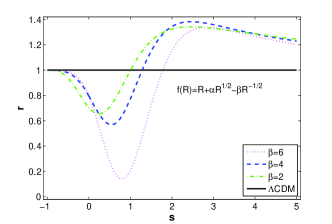
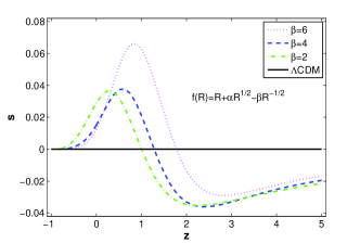
Case 1 $\alpha\neq 0,\beta=0$

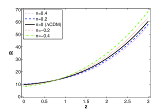
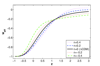
In this case, (19) reduces to

$$f(R)=R-\beta R^{-n}.$$ (20)

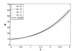
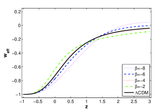
Substituting the form of (20) into Eqs. (16)-(18), with the present fractional matter density $\Omega_{m0}=0.27$, the changing of the Ricci curvature $R$ and the effective equation of state $w_{eff}$ with the redshift $z$ are plotted in Fig.1. It is to be noted that the special case of $(\alpha,n)=(-4.38,0)$ corresponds to the $\Lambda$CDM model. We can easily see that the curvature and the effective equation of state decrease with the evolution of the universe for any choice of $n$. Moreover, the smaller $n$, the faster $R$ decrease, and the larger the present value of $w_{eff}$. Also, the universe turns to an accelerated phase from a decelerated era, and tends to a de Sitter phase in the future.

Figure 1: The figures are for the model $f(R)=R-\beta R^{-n}$ .The left figure is the diagram of Ricci scalar $R$ as a function of redshift $z$. The right figure is the evolution trajectories of $w_{eff}$. Different values of $n$ are selected as $0.4,0.2,0,-0.2,-0.4$ with $\Omega_{m0}=0.27$.

Figure 2: The figures are for the model $f(R)=R+\alpha R^{m}-\beta R^{-n}$ with $m=n=1/2$. The present fractional matter density $\Omega_{m0}=0.27$. The left figure is the diagram of Ricci scalar $R$ as a function of redshift $z$. The right figure is the evolution trajectories of $w_{eff}$.

Figure 3: The figures are for the model $f(R)=R+\alpha lnR+\beta$ .The left figure is the diagram of Ricci scalar $R$ as a function of redshift $z$. The right figure is the evolution trajectories of $w_{eff}$.

Case 2 $\alpha,\beta\neq 0$

In this case, we consider the general form of this type. To study the cosmological behavior of such theories, we adopt the model

$$f(R)=R+\alpha R^{1/2}-\beta R^{-1/2}.$$ (21)

From Fig.2, we clearly find that the curvature and the effective equation of state decrease with the evolution of the universe for any choice of $\beta$. the smaller $\beta$ results in the faster decrease of $R$ and the larger $w_{eff}$ at the present time. It is also obvious that the universe evolves from deceleration to acceleration, and enters to a de Sitter phase in the future.

II.2.2 $f(R)$ theories with logarithm term

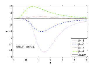
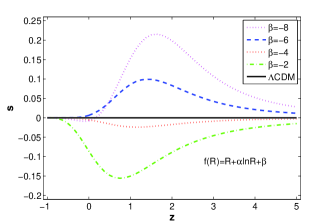
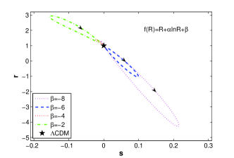
For this type of $f(R)$ theory, we adopt the form

$$f(R)=R+\alpha lnR+\beta,$$ (22)

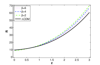
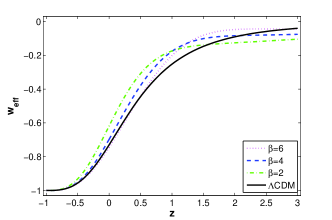
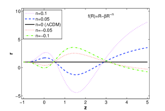
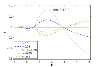
which has been studied in price32 ; price33 . It has been claimed that such theories have a well-defined Newtonian limit price32 . Note that, the asymptotic behavior $\lim_{R\to+\infty}f(R)\to R$ is obtained for any choice of $\alpha$ and $\beta$, and thus, the arbitrary $\alpha$ and $\beta$ can satisfy the assumption that the universe is described by GR at the early time. However, not all combinations of $\alpha$ and $\beta$ can explain a late-time accelerated expansion of the universe. Therefore, for the sake of compatibility with the observational constraints obtained in Sec.4, we select a series values of $\beta$, which can well explain the evolvement of the universe from an early-time deceleration to a late-time acceleration (see Fig.3).

Substituting the form of (22) into Eqs. (16)-(18), with $\Omega_{m0}=0.27$, the changing of the Ricci curvature $R$ and the effective equation of state $w_{eff}$ with the redshift $z$ for this model are plotted in Fig.3. Obviously, $R$ and $w_{eff}$ decrease with the evolution of the universe for any choice of $\beta$. Also, the larger $\beta$ results in the faster decrease of $R$ and the larger $w_{eff}$ at the present time. It is noting that, similar to the result of the above type of theories, the universe evolves from deceleration to acceleration, and enters to a de Sitter phase in the future.

III Statefinder Diagnosis for the Palatini $f(R)$ Gravity

In this section, we turn our attention to the statefinder diagnosis. As we know, two famous geometrical variables characterizing the expansion history of the universe are the Hubble parameter $H=\dot{a}/a$ describing the expansion rate of the universe and the deceleration parameter $q=-\ddot{a}/aH^{2}$ characterizing the rate of acceleration/deceleration of the expanding universe. It is clear that they only depend on the scalar factor $a$ and its derivatives with respect to $t$, i.e., $\dot{a}$ and $\ddot{a}$. However, as the enhancing of cosmological models and the remarkable increase in the accuracy of cosmological observational data, these variables are no longer to be a perfect choice. This can be easily seen from the fact that many cosmological models correspond to the same current value of $q$. As a result, the so-called statefinder diagnosis was introduced in order to discriminate more and more cosmological models.

The statefinder diagnosis is constructed from the scalar $a$ and its derivatives up to the third order. Namely, the statefinder pair $\{r,s\}$ is defined as

$$r\equiv\frac{\dddot{a}}{aH^{3}},\mbox{}\hskip 15.0pts\equiv\frac{r-1}{3(q-1/2)}.$$ (23)

Since different cosmological models exhibit qualitatively different trajectories of evolution in the $s-r$ plane, the statefinder diagnosis is a good tool to distinguish cosmological models. The remarkable property is that the statefinder pair $\{r,s\}=(0,1)$ corresponds to the $\Lambda$CDM model. We can clearly identify the “distance” from a given cosmological model to $\Lambda$CDM model in the $s-r$ plane, such as the quintessence, the phantom, the Chaplygin gas, the holographic dark energy models, the interacting dark energy models, and so forth, which have been shown in the literatures price26 . Particularly, the current values of the parameters $s$ and $r$ in these diagrams can provide a consider way to measure the “distance” from a given model to $\Lambda$CDM model. Generally, according to the reexpression of the deceleration parameter $q$

$$q=-1+(1+z)\frac{H^{\prime}}{H},$$ (24)

where $H^{\prime}\equiv\frac{dH}{dz}$, we can also rewrite the statefinder pair $\{r,s\}$ in terms of the Hubble parameter $H$ and its first and second derivatives $H^{\prime}$ and $H^{\prime\prime}$ with respect to the redshift $z$ as

$$r = 1-2(1+z)\frac{H^{\prime}}{H}+(1+z)^{2}{\frac{H^{\prime}}{H}}^{2}+(1+z)^{2}\frac{H^{\prime\prime}}{H},$$ (25)

$$s = \frac{-2(1+z)H^{\prime}/H+(1+z)^{2}{(H^{\prime}/H)}^{2}+(1+z)^{2}H^{\prime\prime}/H}{3[(1+z)H^{\prime}/H-3/2]}.$$ (26)

(a)

(b)

(c)

Figure 4: $r(z)$ and $s(z)$ for the models $f(R)=R-\beta R^{-n}$, $f(R)=R+\alpha R^{1/2}-\beta R^{-1/2}$ and $f(R)=R+\alpha lnR+\beta$ with $\Omega_{m0}=0.27$.

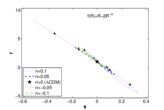
In what follows, we will apply the statefinder diagnosis to the $f(R)$ theories mentioned in Sec.2. The values of parameters we select in such theories are as same as those in the previous section. By describing the evolution trajectories of statefinder parameters $r$ and $s$ for the Palatini $f(R)$ theories, we can differentiate $f(R)$ models from dark energy models, and even discriminate various types of Palatini $f(R)$ theories from each other.

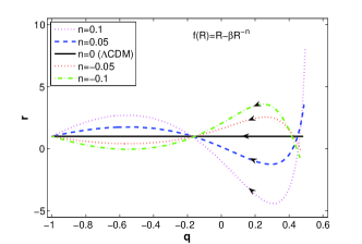
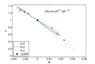
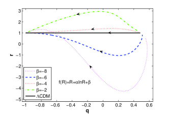
We plot the statefinder parameters $r(z)$ and $s(z)$ for the above two types of Palatini $f(R)$ theories in Fig.4 with $\Omega_{m0}=0.27$. Fig.4 show that $r(z)$ and $s(z)$ for the three models exhibit different features. For the model $f(R)=R-\beta R^{-n}$ (see Fig.4a), the curves cross the $\Lambda$CDM line ($r=1$ or $s=0$) twice times and approach it in the future. Moreover, the curves with $n>0$ start from the region $r>1,s<0$, while the other way round, the curves with $n<0$ start from the region $r<1,s>0$. For the model $f(R)=R+\alpha R^{1/2}-\beta R^{-1/2}$ (see Fig.4b), the curves start from the region $r>1,s<0$, cross the $\Lambda$CDM line and tend to it. While for the model $f(R)=R+\alpha lnR+\beta$ (see Fig.4c), the curves generally do not cross the $\Lambda$CDM line but approach the line in the future. When the parameters $\alpha$ and $\beta$ have the same sign, the curves lie in the region $r>1,s<0$, and in reverse the curves lie in the region $r<1,s>0$ for the case that $\alpha$ and $\beta$ have the opposite sign. From Fig.4, we can clearly find that the behavior of $r(z)$ and $s(z)$ for the models in the Palatini $f(R)$ theories is different from $\Lambda$CDM model and even from other dark energy models. Furthermore, various types of Palatini $f(R)$ theories can be distinguished from each other in the $z-r$ and $z-s$ panels.

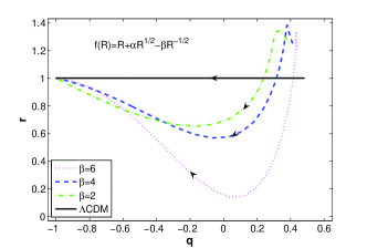
The evolutionary trajectories of the statefinder pairs $\{r,s\}$ and $\{r,q\}$ can also help to differentiate various models in the Palatini $f(R)$ theories from dark energy models. The trajectories $r(s)$ and $r(q)$ for the models under consideration are plotted in Fig.5. It is easy to see from the figure that various models in the palatini $f(R)$ theories in the $s-r$ and $q-r$ planes exhibit the significant differences. Furthermore, the evolutionary trajectories $r(s)$ and $r(q)$ also effectively distinguish the $f(R)$ models from the $\Lambda$CDM model and other dark energy models.

(a)

(b)

(c)

Figure 5: The evolution trajectories of $r(s)$ and $r(q)$ for the models $f(R)=R-\beta R^{-n}$, $f(R)=R+\alpha R^{1/2}-\beta R^{-1/2}$ and $f(R)=R+\alpha lnR+\beta$ with $\Omega_{m0}=0.27$.

IV Numerical Analysis from Observational Data

In order to make $f(R)$ models to be compatible with cosmological observations, we now turn to constrain the parameters in $f(R)$ models with the observational $H(z)$ data.

The Hubble parameter $H(z)$ data depends on the differential ages of the universe as a function of redshift $z$ in the form

$$H(z)=-\frac{1}{1+z}\frac{dz}{dt},$$ (27)

which provides a direct measurement for $H(z)$ through a determination of $dz/dt$ price34 . By using the differential ages of passively evolving galaxies determined from the Gemini Deep Deep Survey (GDDS) price35 and archival data price36 , Simon et al. determined $H(z)$ in the range $0\leq z\leq 1.8$ and used them to constrain the dark energy potential and its redshift dependence price34 . In order to impose constraints on the models of $f(R)$ gravity, we determine the best fit values for the model parameters by minimizing

$$\chi^{2}=\sum_{i=1}^{9}=\frac{[H_{th}(z_{i}|s)-H_{obs}(z_{i})]^{2}}{\sigma^{2}(z_{i})},$$

where $H_{th}(z_{i}|s)$ is the theoretical Hubble parameter at redshift $z_{i}$ given by $(17)$; $H_{obs}(z_{i})$ are the values of the Hubble parameter obtained from the data selected by price34 (SVJ05) and $\sigma(z_{i})$ is the uncertainty for each of the nine determinations of $H(z)$.

IV.1 The Type $f(R)=R+\alpha R^{m}-\beta R^{-n}$

IV.1.1 The Case of $f(R)=R-\beta R^{-n}$

IV.1.2 The Case of $f(R)=R+\alpha R^{m}-\beta R^{-n}$ with $m=n=1/2$

IV.2 The Type $f(R)=R+\alpha lnR+\beta$

V Conclusions and Discussions

In summary, we investigate the $f(R)$ gravity in Palatini formalism by means of the statefinder diagnosis in this paper. Differences of the evolutionary trajectories in the $s-r$ plane among a series of $f(R)$ models have been found. Therefore, the statefinder parameters are powerful to discriminate the models in the Palatini $f(R)$ gravity from dark energy models and even from other $f(R)$ models. Also, the $q-r$ plane has been widely used for discussion on the evolutionary property of the universe. We find that the $f(R)$ models under consideration exhibit different properties in the $q-r$ plane. Since the model parameters are found to be sensitive to the $f(R)$ models, constraining the parameters in the models exactly becomes a valuable task. We use the observational H(z) data to make a combinational constraint.

References

- (1) A.G. Riess et al., Astrophys. J. 116, 1009 (1998); S. Perlmutter et al., Astrophys. J. 517, 565 (1999); J.L. Tonry et al., Astrophys. J. 594, 1 (2003); R.A. Knop et al., Astrophys. J. 598, 102 (2003).
- (2) S. Masi et al., Prog. Part. Nucl. Phys. 48, 243 (2002); D. N. Spergel et al., Astrophys. J. Suppl. 148, 175 (2003); C. L. Bennett et al., Astrophys. J. Suppl. 148, 1 (2003).
- (3) M. Tegmark et al., Phys. Rev. D 69, 103501 (2004); K. Abazajian et al., Astrophys. J. 128, 502 (2004); U. Seljak et al., Phys. Rev. D 71, 103515 (2005).
- (4) V. Sahni and A. Starobinsky, Int. J. Mod. Phys. D 9, 373 (2000); S.M. Carroll, Living Rev. Rel. 4, 1 (2001); P.J.E. Peebles and B. Ratra, Rev. Mod. Phys. 75, 559 (2003); E.J. Copeland, M. Sami and S. Tsujikawa, Int. J. Mod. Phys. D 15, 1753 (2006).
- (5) B. Ratra and P.J.E. Peebles, Phys. Rev. D 37, 3406 (1988); P.J.E. Peebles and B. Ratra, Astrophys. J. 325, L17 (1988); J.P. Ostriker and P.J. Steinhardt, Nature 377, 600 (1995); S.M. Carroll, Phys. Rev. Lett. 81, 3067 (1998); R.R. Caldwell, R. Dave and P.J. Steinhardt, Phys. Rev. Lett. 80, 1582 (1998); N.A. Bahcall, J.P. Ostriker, S. Perlmutter and P.J. Steinhardt, Science 284, 1481 (1999); I. Zlatev, L. Wang and P.J. Steinhardt, Phys. Rev. Lett. 82, 896 (1999); V. Sahni, Class. Quant. Grav. 19, 3435 (2002).
- (6) R.R. Caldwell, Phys. Lett. B 545, 23 (2002); R.R. Caldwell, M. Kamionkowski, N.N. Weinberg, Phys. Rev. Lett. 91, 071301 (2003); P. Singh, M. Sami, N. Dadhich, Phys. Rev. D 68, 023522 (2003); E. Elizalde, S. Nojiri and S.D. Odintsov, Phys. Rev. D 70, 043539 (2004).
- (7) A. Sen, JHEP 0207, 065 (2002); T. Padmanabhan, Phys. Rev. D 66, 021301 (2002); T. Padmanabhan and T.R. Choudhury, Phys. Rev. D 66, 081301 (2002).
- (8) B. Feng, X.L. Wang and X.M. Zhang, Phys. Lett. B 607, 35 (2005); Z.K. Guo, Y.S. Pia, X.M. Zhang and Y.Z. Zhang, Phys. Lett. B 608, 177 (2005); X. Zhang, Commun. Theor. Phys. 44, 762 (2005).
- (9) N. Arkani-Hamed, P. Creminelli, S. Mukohyama and M. Zaldarriaga, JCAP 0404, 001 (2004); F. Piazza and S. Tsujikawa, JCAP 0407, 004 (2004).
- (10) A.Y. Kamenshchik, U. Moschella and V. Pasquier, Phys. Lett. B 511, 265 (2001); M.C. Bento, O. Bertolami and A.A. Sen, Phys. Rev. D 66, 043507 (2002); M.C. Bento, O. Bertolami and A.A. Sen, Phys. Rev. D 70, 083519 (2004).
- (11) C. Csaki, M. Graesser, L. Randall and J. Terning, Phys. Rev. D 62, 045015 (2000).
- (12) C. Brans and R.H. Dicke, Phys. Rev. 124, 925 (1961); R.V. Wagoner, Phys. Rev. D 1, 3209 (1970).
- (13) G.R. Dvali, G. Gabadadze and M. Porrati, Phys. Lett. B 485, 208 (2000);C. Deffayet, G.R. Dvali and G. Gabadadze, Phys. Rev. D 65, 044023 (2002).
- (14) R. Kerner, Gen. Relativ. Gravit. 14, 453 (1982); G. Allemandi, A. Borowiec and M. Francaviglia, Phys. Rev. D 70, 103503 (2004); S.M. Carroll, A.D. Felice, V.Duvvuri, D.A. Easson, M. Trodden and M.S. Turner, Phys. Rev. D 71, 063513 (2005); T.P. Sotiriou and V. Faraoni, gr-qc/0805.1726.
- (15) S.M. Carroll, V. Duvvuri, M. Trodden and M.S. Turner, Phys.Rev. D 70, 043528 (2004).
- (16) A.D. Dolgov and M. Kawasaki, Phys. Lett. B 573, 1 (2003); M.E. Soussa and R.P. Woodard, Gen. Rel. Grav. 36, 855 (2004); S. Nojiri and S.D. Odintsov, Int. J. Geom. Meth. Mod. Phys. 4, 115 (2007); R.P. Woodard, Lect. NotesPhys. 720, 403 (2007).
- (17) X. Meng and P. Wang, Class. Quant. Grav. 20, 4949 (2003); X. Meng and P. Wang, Class. Quant. Grav. 21, 951 (2004).
- (18) T. Chiba, Phys. Lett. B 575, 1 (2003); L. Amendola and S. Tsujikawa, Phys. Lett. B 660, 125 (2008).
- (19) X. Meng and P. Wang, Gen. Rel. Grav. 36, 1947 (2004); T.P. Sotiriou, Phys. Rev. D 73, 063515 (2006); T.P. Sotiriou, Gen. Rel. Grav. 38, 1407 (2006).
- (20) L. Amendola, D. Polarski and S. Tsujikawa, Phys. Rev. Lett. 98, 131302 (2007); L. Amendola, D. Polarski and S. Tsujikawa, Int. J. Mod. Phys. D 16, 1555 (2007);
- (21) L. Amendola, R. Gannouji, D. Polarski and S. Tsujikawa, Phys. Rev. D 75, 083504 (2007).
- (22) T. P. Sotiriou, Gen. Rel. Grav. 38, 1407 (2006).
- (23) M. Amarzguioui, O. Elgaroy, D.F. Mota and T. Multamaki, Astron. Astrophys. 454, 707 (2006); S. Fay, R. Tavakol and S. Tsujikawa, Phys. Rev. D 75, 063509 (2007).
- (24) J.A.R. Cembranos, Phys. Rev. D 73, 064029 (2006); V. Faraoni, Phys. Rev. D 74, 104017 (2006).
- (25) V. Sahni, T.D. Saini, A.A. Starobinsky and U. Alam, JETP Lett. 77, 201 (2003).
- (26) U. Alam, V. Sahni, T.D. Saini and A.A. Starobinsky, Mon. Not. Roy. Astron. Soc. 344, 1057 (2003); X. Zhang, Phys. Lett. B 611, 1 (2005); X. Zhang, Int. J. Mod. Phys. D 14, 1597 (2005); P.X. Wu and H.W. Yu, Int. J. Mod. Phys. D 14, 1873 (2005); B.R. Chang, H.Y. Liu, L.X. Xu, C.W. Zhang and Y.L. Ping, JCAP 0701, 016 (2007); M.R. Setare, J.F. Zhang and X. Zhang, JCAP 0703, 007 (2007); Z.L. Yi and T.J. Zhang, Phys. Rev. D 75, 083515 (2007); H. Wei, R.G. Cai, Phys. Lett. B 655, 1 (2007); J.F. Zhang, X. Zhang and H.Y. Liu, Phys. Lett. B 659, 26 (2008); D.J. Liu, W.Z. Liu, Phys. Rev. D 77, 027301 (2008); S. Li, Y.G. Ma and Y. Chen, Int. J. Mod. Phys. D 18, 1785 (2009).
- (27) N.W. Halverson, E.M. Leitch, C. Pryke, J. Kovac, J.E. Carlstrom, W.L. Holzapfel, M. Dragovan, J.K. Cartwright, B.S. Mason, S. Padin, T.J. Pearson, M.C. Shepherd and A.C.S. Readhead, ApJ. 568, 38 (2002).
- (28) C.B. Netterfield, P.A.R. Ade, J.J. Bock, J.R. Bond, J. Borrill, A. Boscaleri, K. Coble, C.R. Contaldi, B.P. Crill, P. de Bernardis, P. Farese, K. Ganga, M. Giacometti, E. Hivon, V.V. Hristov, A. Iacoangeli, A.H. Jaffe, W.C. Jones, A.E. Lange, L. Martinis, S. Masi, P. Mason, P.D. Mauskopf, A. Melchiorri, T. Montroy, E. Pascale, F. Piacentini, D. Pogosyan, F. Pongetti, S. Prunet, G. Romeo, J.E. Ruhl and F. Scaramuzzi, Astrophys. J. 571, 604 (2003).
- (29) M. Amarzguioui, O. Elgaroy, D. F. Mota and T. Multamaki, Astron. Astrophys. 454, 707 (2006).
- (30) T.P. Sotiriou, Phys. Rev. D 73, 063515 (2006).
- (31) X.H. Meng and P. Wang, Class. Quant. Grav. 21, 2029 (2004).
- (32) S. Nojiri and S.D. Odintsov, Gen. Rel. Grav. 36, 1765 (2004).
- (33) X.H. Meng and P. Wang, Phys. Lett. B 584, 1 (2004).
- (34) J. Simon, L. Verde and R. Jimenez, Phys. Rev. D 71, 123001 (2005).
- (35) R.G. Abraham et al. [GDDS Collaboration], Astron. J. 127, 2455 (2004).
- (36) T. Treu, M. Stiavelli, S. Casertano, P. Moller and G. Bertin, Mon. Not. Roy. Astron. Soc. 308, 1037 (1999); T. Treu, M. Stiavelli, P. Moller, S. Casertano and G. Bertin, Mon. Not. Roy. Astron. Soc. 326, 221 (2001); T. Treu, M. Stiavelli, S. Casertano, P. Moller and G. Bertin, Astrophys. J. Lett. 564, L13 (2002); J. Dunlop, J. Peacock, H. Spinrad, A. Dey, R. Jimenez, D. Stern and R. Windhorst, Nature 381, 581 (1996); H. Spinrad, A. Dey, D. Stern, J. Dunlop, J. Peacock, R. Jimenez and R. Windhorst, Astrophys. J. 484, 581 (1997); L.A. Nolan, J.S. Dunlop, R. Jimenez and A.F. Heavens, Mon. Not. Roy. Astron. Soc. 341, 464 (2003).
- (37) A. Ali, R. Gannouji, M. Sami and A.A. Sen, arXiv:astro-ph/1001.5384.