Spectral Lag Relations in GRB Pulses Detected with HETE-2

Abstract

Using a pulse-fit method, we investigate the spectral lags between the traditional gamma-ray band (50$-$400 keV) and the X-ray band (6$-$25 keV) for 8 GRBs with known redshifts (GRB 010921, GRB 020124, GRB 020127, GRB 021211, GRB 030528, GRB 040924, GRB 041006, GRB 050408) detected with the WXM and FREGATE instruments aboard the HETE-2 satellite. We find several relations for the individual GRB pulses between the spectral lag and other observables, such as the luminosity, pulse duration, and peak energy $E_{\rm peak}$. The obtained results are consistent with those for BATSE, indicating that the BATSE correlations are still valid at lower energies (6$-$25 keV). Furthermore, we find that the photon energy dependence for the spectral lags can reconcile the simple curvature effect model. We discuss the implication of these results from various points of view.

1 Introduction

Gamma-Ray Bursts (GRBs) are the most energetic explosions in the universe. Past studies have found that GRBs consist of ultra-relativistic outflows with collimated jets at cosmological distances. However, it is not clear how the central engine forms and how the electrons or protons are accelerated in shocks and photons are radiated. In addition, GRBs are quite important as candidates for distance-indicators. Owing to their very intense brightness, GRBs can be a powerful tool to measure distances in the high redshift universe.

One of the characteristics of GRB prompt emission is the spectral lag, which is the time delay in the arrival of lower-energy emission relative to higher-energy emission. The previous analyses have been done using a sample of many BATSE GRBs between typical energy bands 25$-$50 keV and 100$-$300 keV, using both CCF (cross correlation function; e.g., [Norris et al. (2000)]) and peak-to-peak difference (e.g., [Hakkila et al. (2008)]). An anti-correlation between the spectral lag and the luminosity exists for the BATSE GRBs above 50 keV energies. Since we can obtain the intrinsic luminosity of GRBs from the lag-luminosity relation once we measure the spectral lag, the distance of the GRBs can be derived from the observed flux. But it is not clear whether the relation is valid in wider energy bands. In addition, from the results of [Hakkila et al. (2008)], it is shown that the spectral lag characterizes each pulse rather than the entire burst.

From the theoretical point of view (e.g., [Qin et al. (2004)]), the rise phase timescale may be responsible for the intrinsic pulse width, while the decay phase timescale may be determined by geometrical effects (e.g., the curvature effect). The curvature effect ([Qin (2002)], [Qin & Lu, (2005)], [Lu et al. (2006)]) arises from relativistic effects in a sphere expanding with a high bulk Lorentz factor $\Gamma$ = 1/(1 - $\beta^{2}$)^1/2 $\sim$ 100. Because of the curvature of the emitting shell, there will be a time delay between the photons emitted simultaneously in the comoving frame from different points on the surface. However, [Zhang et al. (2007)] showed that the curvature effect alone is not enough to explain energy-dependent pulse properties obtained from the systematic analysis of lag and temporal evolution. Alternative models are the off-axis model proposed by [Ioka & Nakamura (2001)]　and the time-evolution of shock propagation ([Daigne & Mochkovitch (1998)], [Daigne & Mochkovitch (2003)], [Bošnjak et al. (2009)]) may also reproduce the spectral lag and the lag-luminosity relation. Thus, it is not clear that either the curvature effect or other effects cause the spectral lag. While the curvature effect should necessarily affect the pulse profile, the time-evolution of shock propagation or off-axis model strongly depends on unknown model parameters.

In this paper, in order to unveil the properties of the spectral lag for each pulse, we investigate the HETE-2 sample with a wider energy range especially at the low-energy end ($>$2 keV) than the BATSE sample. In sections 2 and 3 we explain the sample selection and the pulse-fit method. In section 4, we describe the result of the obtained relations between the spectral lag and other observables, and we discuss a detailed energy dependence for the spectral lag in section 5. Finally, we briefly comment on the future prospects in section 6.

2 HETE-2 Sample and Selection

HETE-2 had two scientific instruments on-board which are relevant to our study: the FREnch GAmma-ray TElescope (FREGATE), which gave the trigger for GRBs and performed spectroscopy over a wide energy range (6$-$400 keV); and the Wide-field X-ray Monitor (WXM), which was the key instrument to localize GRBs to $\sim$10^′, and sensitive to the 2$-$25 keV energy range, lower than the FREGATE one. The instruments have two types of data. The survey data were recorded with fixed energy bands and time resolution whenever the instruments were on. The time-tagged data were produced with a fixed duration (several minutes) when the instruments were triggered by bursts. From the time-tagged data, we can produce light curves in arbitrary energy bands, while the BATSE detector in general created light curves only in fixed energy bands (Although the BATSE detector actually has time-tagged data, many BATSE GRBs are not fully covered due to the limitation of the memory size for the time-tagged data.).

We perform the spectral-lag analysis using a sample of 8 GRBs detected by HETE-2 with known or estimated redshifts for the study of the lag-luminosity relation in section 4. Our selection criteria for the GRB samples are the following: 1) $T_{90}$ $>$ 2 s, where $T_{90}$ is the observed duration including 90% of the total observed counts, and 2) time-tagged data are available. For the latter, we note that the time-tagged data were lost for some bursts due to downlink problems or invalidation of the instruments (e.g., GRB030328, GRB030329 etc.). For these bursts, since the available energy band is too coarse for the survey data (e.g., 6$-$40 keV, 6$-$80 keV, and 32$-$400 keV for FREGATE), we cannot conduct a detailed study of the spectral lag. For the analysis in section 4, we use the FREGATE instrument alone because off-axis photon events were partially coded and the number of events detected by the WXM instrument was often small, while the FREGATE instrument detected more photons compared to those of the WXM instrument due to its relatively large effective area ($\sim$150 cm²); not all the selected GRBs have enough photons to perform the analysis in the WXM energy band.

In addition, for studying the detailed energy dependence of the spectral lag for individual GRB pulses in section 5, we add 2 GRBs without known redshifts having sufficiently non-overlapped pulses to the sample. In this analysis, we use not only the FREGATE instrument but also the WXM instrument, because some GRBs have good enough statistics detected by the WXM instrument. Here, since there are not good statistics in the multiple energy bands for GRB 020124 and GRB 041006, we exclude the GRBs from the sample.

We show the list of 10 GRBs in Table 1 and the energy bands in the burst rest frame which are covered by the WXM and FREGATE instruments for the selected GRBs with known redshifts in Fig. 1.

Table 1: GRB samples

GRB	redshift	Reference
010921	0.45	[Djorgovski et al. (2001)]
020124	3.20	[Hjorth et al. (2003)]
020127	1.91	[Berger et al. (2007)]
021211	1.01	[Vreeswijk et al. (2003)]
030528	0.78	[Rau et al. (2005)]
030725	-	[Pugliese et al. (2005)]
040924	0.86	[Wiersema et al. (2004)]
041006	0.72	[Stanek et al. (2005)]
050408	1.24	[Berger et al. (2005)]
060121	-	[de Ugarte Postigo et al. (2006)]

¹: this is a possible value estimated from the afterglow investigation and spectral energy distribution.

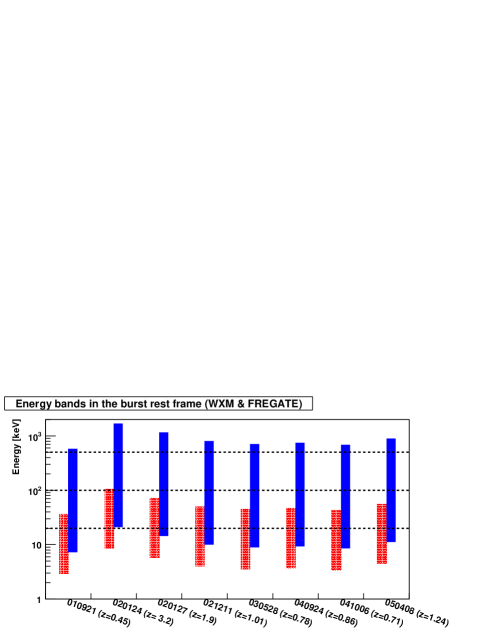
Figure 1: Energy bands in the burst rest frame for the selected GRBs. The red dotted bars represent the WXM bands and the blue solid ones represent the FREGATE bands. The adopted energy ranges are the range between the dashed lines (20$-$100 keV and 100$-$500 keV).

3 Method

Each GRB pulse is fitted with a four-parameter pulse model (Norris et al., 2005), if $t$ $>$ $t_{\rm start}$

$$I(t) = A\lambda\exp{(-\tau_{1}/(t-t_{\rm start})-(t-t_{\rm start})/\tau_{2})}+B(t)$$ (2)

$$= A\lambda\exp(-\tau_{1}/(t+\tau_{\rm peak}-t_{\rm peak})$$

$$-(t+\tau_{\rm peak}-t_{\rm peak})/\tau_{2})+B(t)$$

and if $t$ $<$ $t_{\rm start}$, $I(t)=B(t)$ , where $I$ is the intensity, $t$ is the time after the trigger, $\tau_{1}$ and $\tau_{2}$ are the pulse rise and pulse decay constants, $\lambda\equiv\exp{\left(2(\tau_{1}/\tau_{2})^{1/2}\right)}$, $t_{\rm peak}$ is the time of the pulse’s maximum intensity $A$, $t_{\rm start}$ is the start time, $\tau_{\rm peak}\equiv(\tau_{1}\tau_{2})^{1/2}$ is the peak time from the start time $t_{\rm start}$, so that $t_{\rm peak}=t_{\rm start}+\tau_{\rm peak}$, and $B(t)$ is the background function (we utilize a constant or linear function). In Eq. 2, $t_{\rm peak}$ is treated as a primary fitting parameter in order to estimate the uncertainty in $t_{\rm peak}$ directly in the fitting procedure.

The time $t_{\rm start}$ is the formal onset time and in some cases $t_{\rm start}$ is not indicative of the visually apparent onset time. Especially in the case of $\tau_{1}\gg 1$ s, $t_{\rm start}$ is extremely far from the peak of the pulse. Here, as described in Norris et al. (2005), we introduce an effective onset time $t_{\rm eff}$ arbitrarily defined as the time when the pulse reaches 0.01 times the peak intensity. Furthermore, the values of $t_{\rm eff}$ are different in different energy bands. For HETE-2 GRBs, the statistics of GRBs are not as good as those of BATSE because, e.g., the effective area of the FREGATE detector ($\sim$ 150 cm²) is lower by a factor of $\sim$ 10 than that of the BATSE detector ($\sim$ 2000 cm²). This causes $t_{\rm eff}$ to be scattered in different energy bands due to the uncertainties in the determination of $\tau_{1}$ and $\tau_{2}$. To avoid this, we adopt an onset time of the “bolometric” light-curve profile, $t_{\rm eff}^{\prime}$, derived by fitting the light curve in the 6 $-$ 400 keV band, which corresponds to the entire FREGATE-energy band. The adoption of $t_{\rm eff}^{\prime}$ is supported by Hakkila & Nemiroff (2009). They showed that the onset of GRB pulses occurs simultaneously across all energy bands. Thus, we define $T_{\rm peak}$ = $t_{\rm peak}-t_{\rm eff}^{\prime}$ in this paper. The corresponding uncertainties are calculated using the error propagation formula.

Spectral peak lags are defined as the difference between the maximum-intensity times in different energy bands as

$$\tau_{\rm lag}\equiv t_{\rm peak,low}-t_{\rm peak,high},$$ (3)

where “low” and “high” represent the low and high energy bands, respectively. Another measurable pulse property is the pulse duration $w\equiv 3\tau_{2}{(1+4\sqrt{\tau_{1}/\tau_{2}}/3)}^{1/2}$ defined as the time intervals where intensities are equal to $e^{-3}I(t_{\rm peak})$.

4 Relation between the Spectral Lag and Other Parameters

In this paper, we adopt two sets of energy bands in order to calculate the spectral lag between the two divided bands. The first one is 6$-$25 keV and 50$-$400 keV in the observer’s frame. Although in the previous study by BATSE the energy bands between 25$-$50 keV and 100$-$300 keV had been adopted, we adopt the lower energy band ($<$25 keV) and test if the same relation (e.g., lag-luminosity relation) is established or not. Furthermore, for all the previous studies of the spectral lag the energy bands refer to the observer’s frame. However if the spectral lag is a characteristic property of GRBs, it is better to derive the spectral lags between the energy bands in the burst rest frame. The HETE-2 time-tagged data have an advantage for such an analysis, compared with the BATSE detector. Thus we adopt energy bands 20$-$100 keV and 100$-$500 keV in the burst rest frame to be covered by the FREGATE instrument. The adopted energy bands are shown as horizontal lines in Fig. 1.

Here we use pulses that satisfy the following requirements: the significance of the spectral lag $\sigma_{\rm sig}>1.5$ and positive lag $\tau_{\rm lag}>0$, where

$$\sigma_{\rm sig} \equiv \tau_{\rm lag}/\sigma_{\rm lag},$$ (4)

$$\sigma_{\rm lag} \equiv \left(\sigma_{\rm peak,low}^{2}+\sigma_{\rm peak,high}^{2}\right)^{1/2}.$$ (5)

The value $\sigma_{\rm lag}$ represents the 1-$\sigma$ uncertainty of $\tau_{\rm lag}$ and $\sigma_{\rm peak}$ is defined as the 1-$\sigma$ uncertainty of $t_{\rm peak}$. For the negative lag, its significance is low ($\sigma_{\rm lag}<1$) and the number of pulses having a negative lag is very small, and we do not take it into account. One of the pulse-fitted results is shown in Fig. 2 (GRB 050408) using the $\chi^{2}$ fitting routine. For the fitting, we fit pulses to make the obtained values of $\chi^{2}$/d.o.f. (degree of freedom) reasonable ($\sim$1).

(80mm,80mm)figure02.eps

Figure 2: Pulse fit for GRB 050408 in the 6-25 keV and 50-400 keV bands in the observer’s frame.

4.1 Observer’s frame

First, we show the scatter plots of the spectral lag $\tau_{\rm lag}$ and luminosity $L_{\rm iso}$ in the top left panel of Fig. 3 where the spectral lag is calculated in the observer’s frame. The luminosity in this paper is defined as the average luminosity over the pulse FWHM timescale.

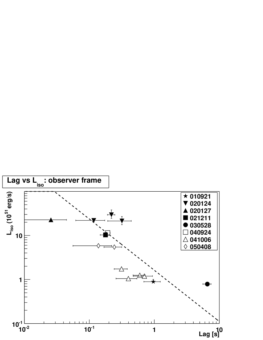
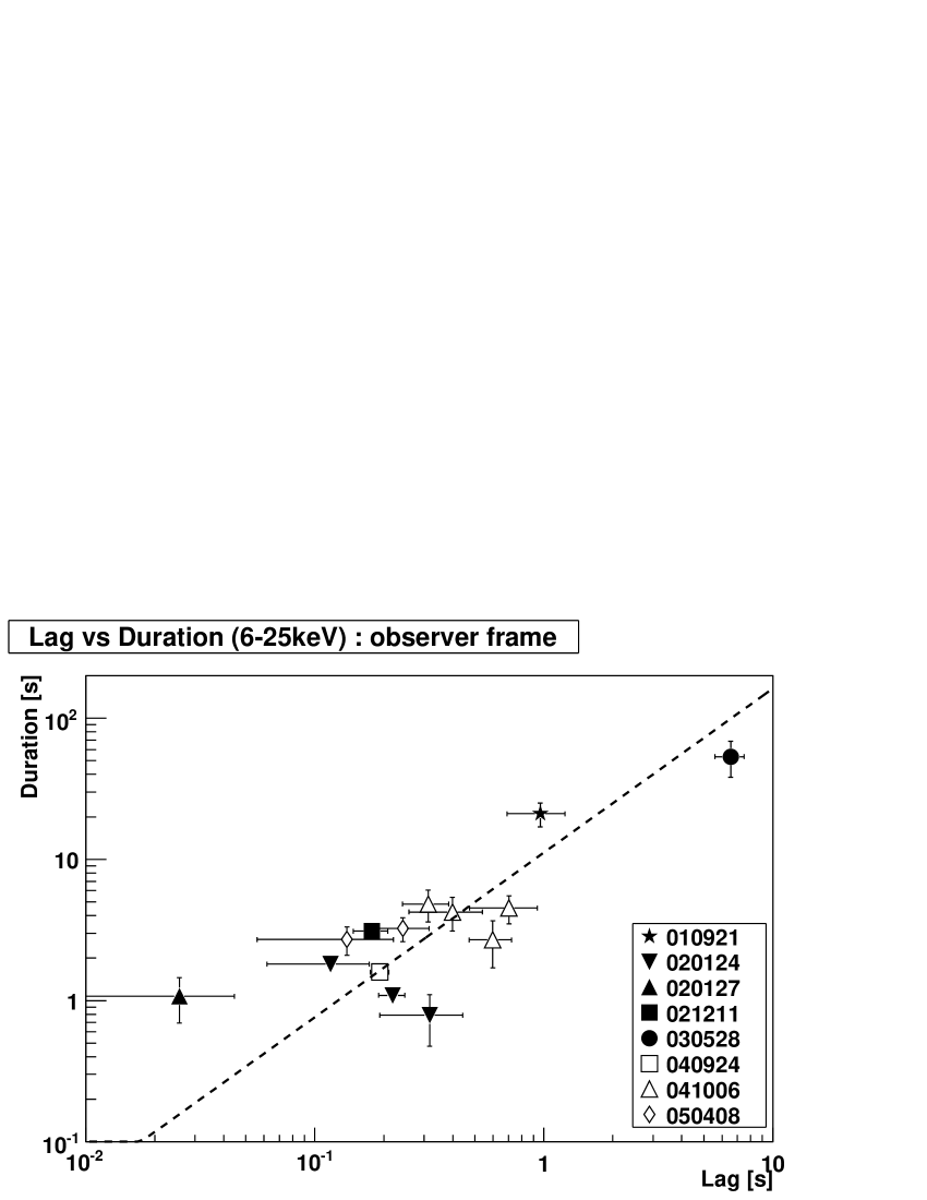
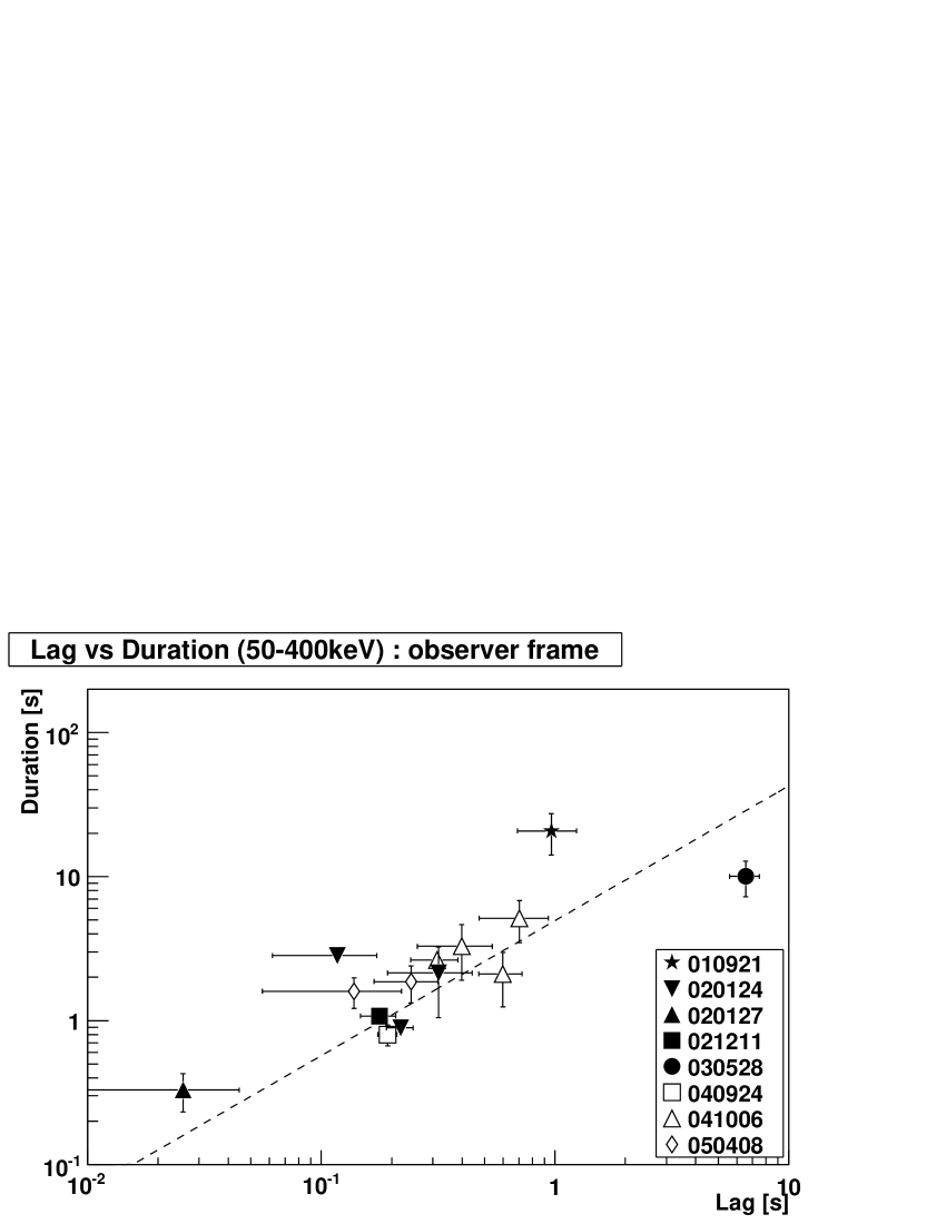
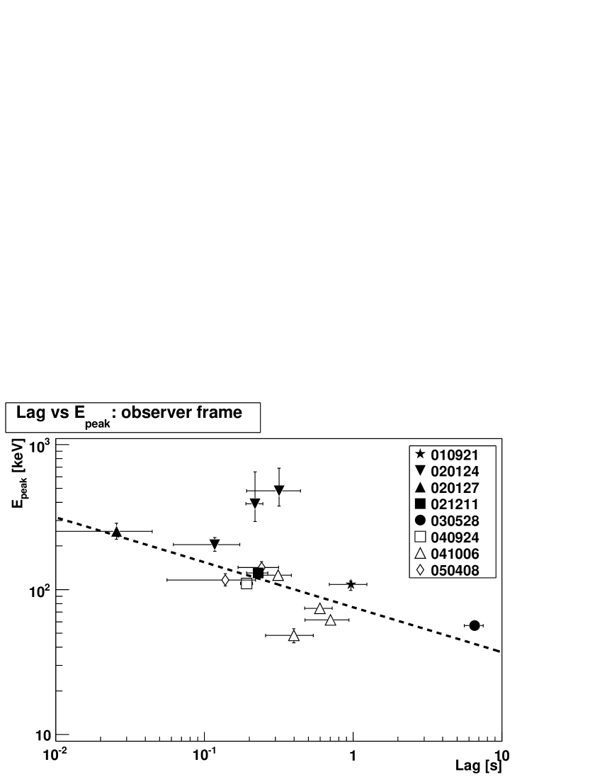
Figure 3: Scatter plot (observer’s frame) of spectral lag vs. luminosity (top left), duration for the low-energy band (top right), duration for the high-energy band (bottom left), and $E_{\rm peak}$ (bottom right). The dashed lines represent the best-fit functions.

As shown in this figure, we can see an anti-correlation between the spectral lag and the luminosity. Here, for the correlation coefficient, we adopt the Spearman rank-order correlation test. Furthermore, to estimate the correlation coefficient on the basis of the spectral lag’s confidence level, we perform a Monte Carlo simulation. Since we have already obtained $\tau_{\rm lag}$, $\sigma_{\rm lag}$, the luminosity and its uncertainty, we can generate a pseudo plot based on the specific probability distributions, that is, make a plot similar to the top left panel of Fig. 3 with random number seeds. Then we calculate the value of the correlation coefficient $R$ for the generated pseudo plot using the Spearman rank-order correlation test. Finally we repeat the same procedure 10000 times with different random number seeds. As we obtain the histogram of the correlation coefficient, we regard the 1-$\sigma$ width as the 1-$\sigma$ confidence level. We adopt this method in the following analysis.

For the lag-luminosity relation in the observer’s frame, we obtain the correlation coefficients as $R$ = -0.79${}^{+0.16}_{-0.05}$ with a chance probability of 7.7 $\times$ 10^-4 at the most probable value. The best-fit functional form is $\log(L_{51})=A_{1}+B_{1}\log(\tau_{\rm lag})$ with $A_{1}=-0.79\pm 0.04,B_{1}=-1.16\pm 0.07$; the reduced chi-square is 133.2/12 in the observer’s frame. Although there are large scatters in the data from the best-fit line, the lag-luminosity relation holds even for the low energy band ($<$ 25 keV). While our results reconfirm the lag-luminosity relation previously reported, our spectral lag index (-1.2) is slightly smaller than that of Hakkila et al. (2008) (index $\sim$-0.6). The slight difference seems to come from the following: (1) the different timescales to estimate the luminosity (BATSE used 256 ms, while we adopt the pulse FWHM timescale), (2) the small numbers of GRB samples for both Hakkila et al. (2008) and HETE-2, and (3) the difference in the adopted energy band and/or the instrumental response between Hakkila et al. (2008) and ours. Thus, the slight difference in the power-law index of the correlations between Hakkila et al. (2008) and our results is not surprising.

We show the scatter plots of the spectral lags and the durations at low and high energies in the top right and bottom left panels of Fig. 3, respectively. We find correlations between the spectral lags and durations in both the 6$-$25 keV and 50$-$400 keV bands. The best-fit functional form of these relations is $\log(w_{\rm low})=A_{2}+B_{2}\log(\tau_{\rm lag})$ with $A_{2}=1.05\pm 0.06,B_{2}=1.16\pm 0.09$ and the reduced chi-square is 43.0/12 in the 6$-$25 keV band and $\log(w_{\rm high})=A_{3}+B_{3}\log(\tau_{\rm lag})$ with $A_{3}=0.69\pm 0.05,B_{3}=0.94\pm 0.08$, and 45.1/12 in the 50$-$400 keV band. The correlation coefficients are $R$ = 0.66${}^{+0.10}_{-0.14}$ and $R$ = 0.74${}^{+0.06}_{-0.14}$, and the corresponding chance probabilities at the most probable values are 1.0 $\times$ 10^-2 and 2.5 $\times$ 10^-3 in the 6$-$25 keV and 50$-$400 keV bands, respectively. The low chance probabilities assure the tight correlations. These results are almost consistent with those of Hakkila et al. (2008) (index 0.85).

Finally, the scatter plot of the spectral lag and peak-time $E_{\rm peak}$ is shown in the bottom right panel of Fig. 3 in the observer’s frame . The best-fit functional form is $\log(E_{\rm peak})=A_{4}+B_{4}\log(\tau_{\rm lag})$ with $A_{4}=1.88\pm 0.02,B_{4}=-0.31\pm 0.02$ and the reduced chi-square is 97.8/12. The correlation coefficient is $R$ = -0.66${}^{+0.15}_{-0.08}$ with chance probability 1.0 $\times$ 10^-2. Thus, we obtain a possible anti-correlation between $E_{\rm peak}$ and the spectral lag, though the dependence of the spectral lag on $E_{\rm peak}$ is relatively weak (index $\sim$ -0.3 ) compared with the other parameters.

4.2 Burst Rest frame

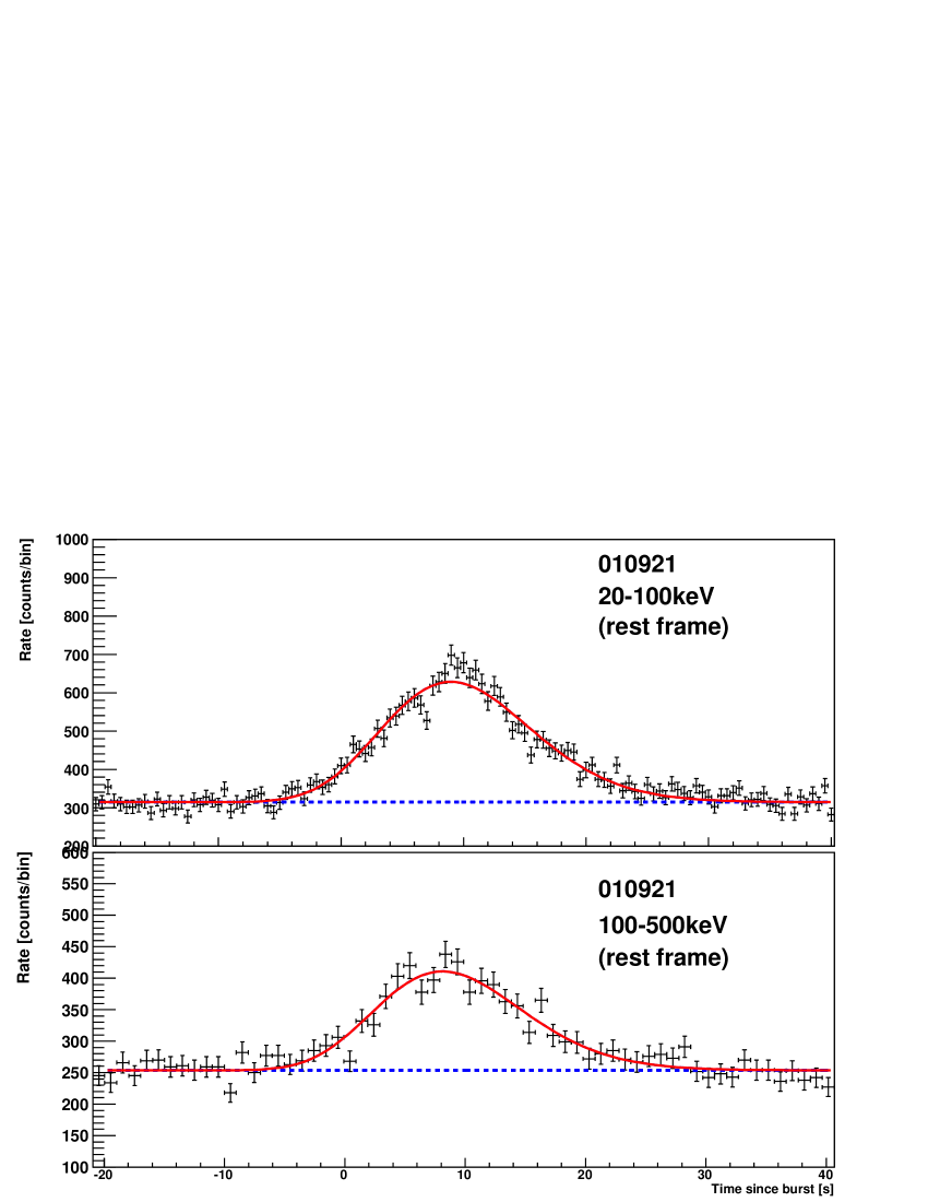
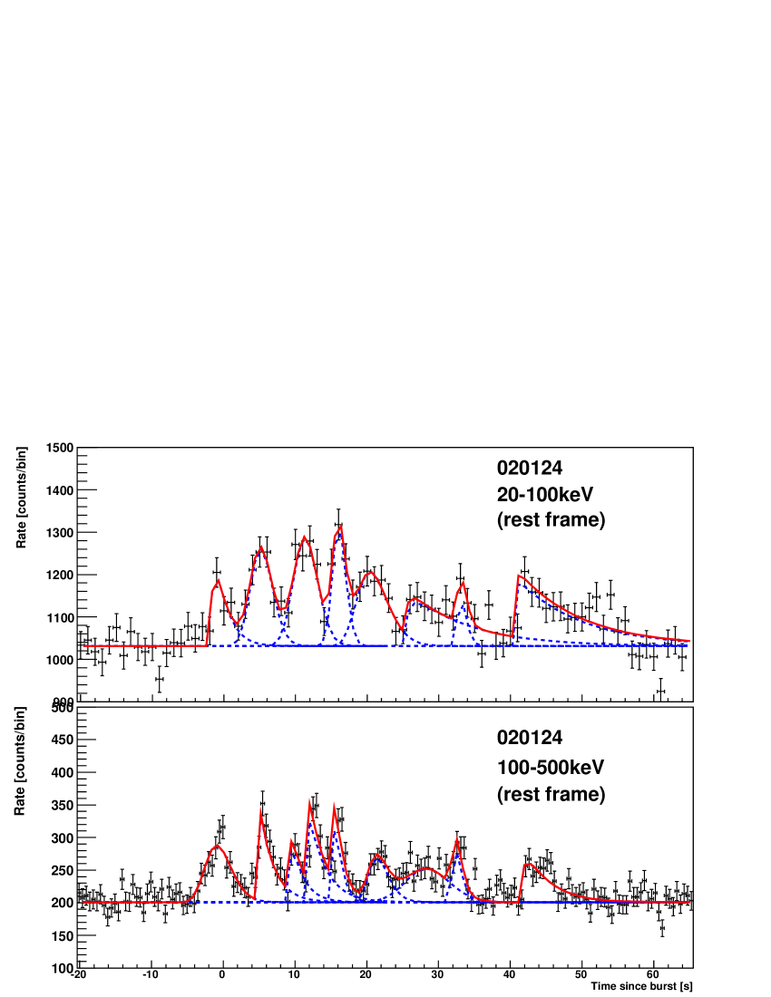
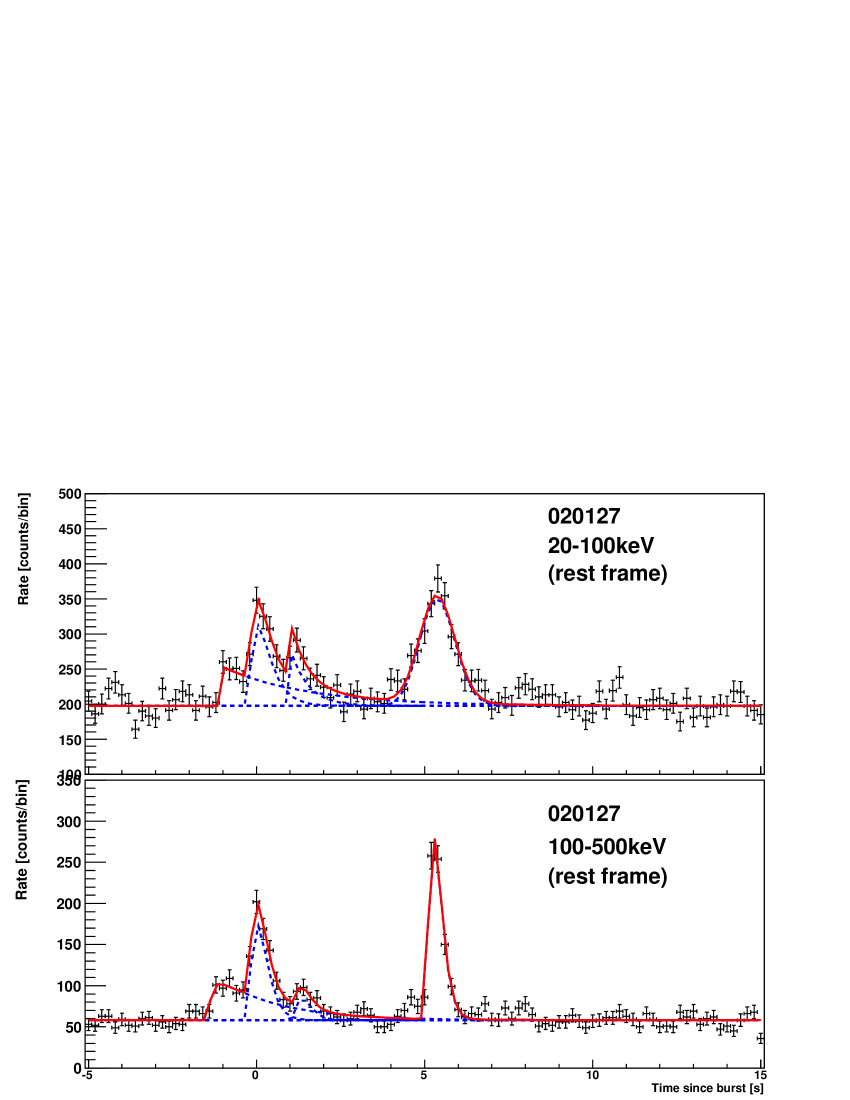
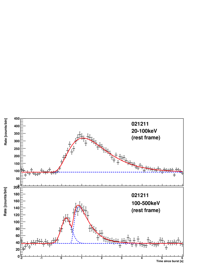
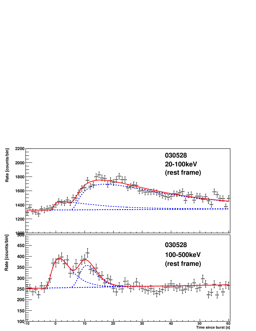
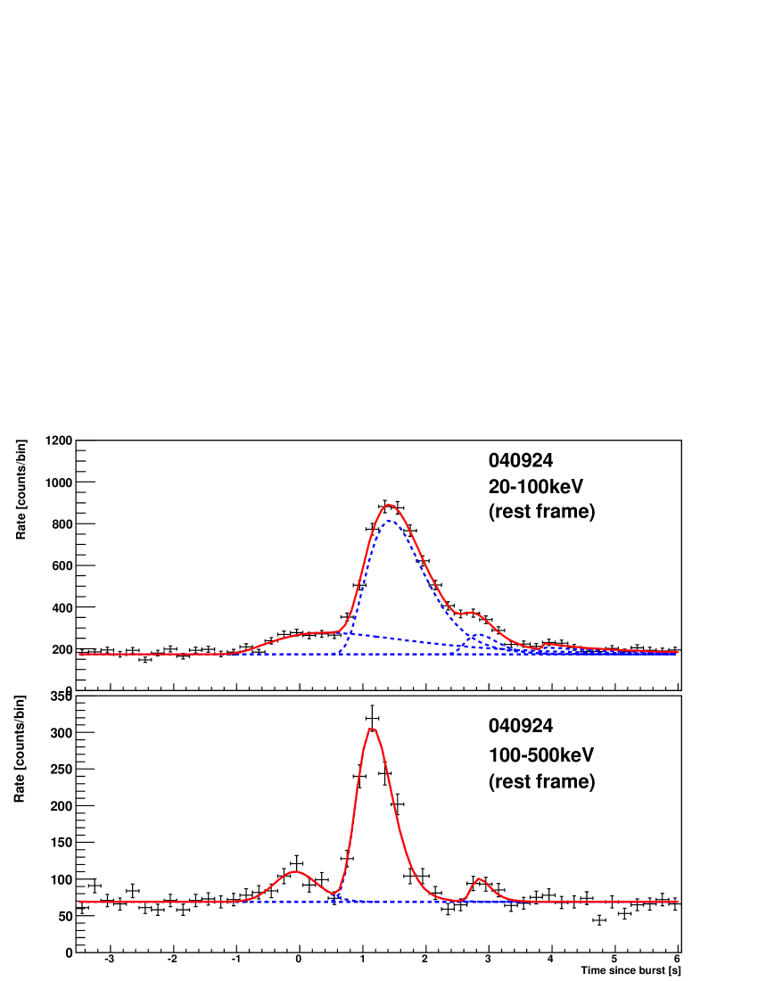
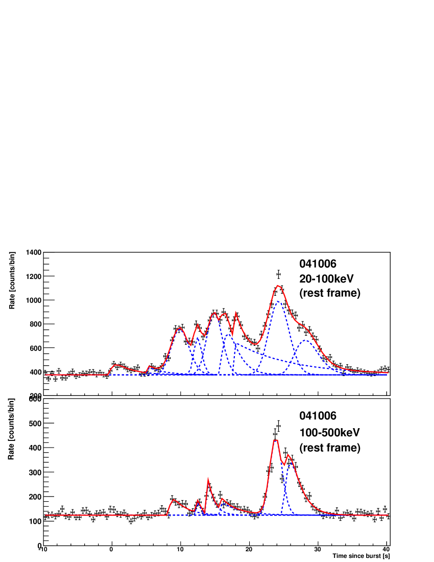
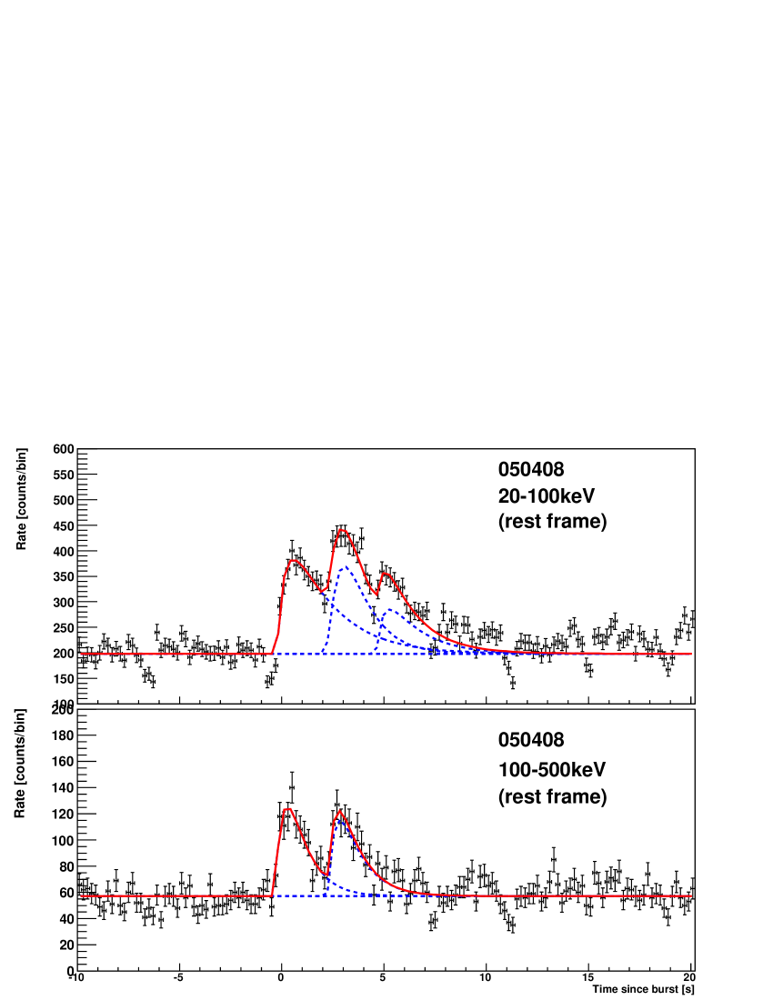
Figure 8: The result of the fitted pulses in the burst rest frame (20$-$100 keV and 100$-$500 keV).

We show the results of the relations between the spectral lag and other parameters in the burst rest frame in Fig. 4 (The result of the fitted pulses is shown in Fig. 8), and the adopted energy bands are determined to have the same energies in common (20$-$100 keV and 100$-$500 keV). As is the case for the observer’s frame, the best-fit parameters of each relation are summarized in Table 2. We find that there is no significant difference in results between the observer’s frame and the burst rest frame. The obtained results support the idea that the cosmological effects should not significantly change our measurement in the observer’s frame even though most GRBs are found at high redshifts. The intrinsic properties for GRB pulses predominate over the cosmological effects as suggested by Hakkila et al. (2008) and Hakkila & Cumbee (2009).

4.3 Discussion

We have obtained the correlation between the spectral lag and duration, $L_{\rm iso}$ and $E_{\rm peak}$ in the observer’s and the burst rest frames. In particular, our result extends the energy coverage to a lower energy band (6$-$25 keV). This indicates that the GRB emission in the wide X-ray band has the same origin.

As there is no significant difference between the results in the observer’s and burst rest frames, it is natural to adopt the burst rest frame to discuss the origin of the spectral lag. Thus, in the following discussion, we refer to the case of the burst rest frame.

4.3.1 Physical Origin of the Relations

To account for the relation between the spectral lag and $L_{\rm iso}$, let us consider the off-axis model suggested by Ioka & Nakamura (2001); the detector observes a GRB jet with different viewing angles $\theta_{v}$. The intrinsic physical parameters, bulk Lorentz factor $\Gamma$, opening half-angle $\Delta\theta\sim 1/\Gamma$, shell radius $r_{0}$ from the center, and $E_{\rm peak}^{\prime}$ in the comoving frame are assumed to be the same for all GRBs. In this paper, we adopt the same parameters as those of Ioka & Nakamura (2001); $\Gamma\Delta\theta$ = 1, $r_{0}/c\beta\Gamma^{2}$ = 1. This model assumes an intrinsic spectral shape in the comoving frame which is approximated by the Band function (Band et al., 1993) as

$$f(E^{\prime})=\left(\frac{E^{\prime}}{E_{0}}\right)^{1+\alpha_{B}}\left[1+\left(\frac{E^{\prime}}{E_{0}}\right)^{s}\right]^{\frac{\beta_{B}-\alpha_{B}}{s}}$$ (6)

where $\alpha_{B}$ and $\beta_{B}$ are the low- and high-energy indices, $s$ describes the smoothness of the transition between the high and low energies and $E_{0}$ is the break energy. Ioka & Nakamura (2001) showed that the observable values such as luminosity, the pulse duration (FWHM) $w$, and the peak energy $E_{\rm peak}$, change with the viewing angle $\theta_{v}$ and correlate with the spectral lag as,

$$L_{\rm iso} \propto \tau_{\rm lag}^{\frac{-2+\alpha_{B}}{s+1}},$$ (7)

$$w \propto 1+{\rm const}\times\tau_{\rm lag}^{\frac{1}{s+1}},$$ (8)

$$E_{\rm peak} \propto \left(1+{\rm const}\times\tau_{\rm lag}^{\frac{1}{s+1}}\right)^{-1}$$ (9)

We have obtained $\L_{\rm iso}\propto\tau_{\rm lag}^{-1.2}$ from the lag-luminosity relation in Fig. 4 so that the off-axis model with $s=1.5$ and the typical value for the low-energy photon index $\alpha_{B}=-1$ can reproduce the lag-luminosity relation.

The expected theoretical results are superimposed on Fig. 4. Here, we adopt arbitrary normalization values for the theoretical lines. For the lag-duration relation in the high-energy band (100$-$500 keV), the observational points are consistent with the theoretical curve. For the lag-duration relation in the low-energy band (20$-$100 keV), the observational points agree with the theoretical curve for small spectral lags, although there are some outliers for large spectral lags. For the lag-$E_{\rm peak}$ relation, we find a consistency between the observational points and the theoretical curve. Except for some outliers, we find that the off-axis model can explain the observational results well, even though the model seems to be oversimplified. (All intrinsic physical parameters are common for all GRBs in this model.) Furthermore, for the off-axis model the spectral lag is calculated using the difference between the peak times in the different energy bands just as we calculate the spectral lag, unlike Norris et al. (2000), in which the spectral lags are calculated using the CCF method.

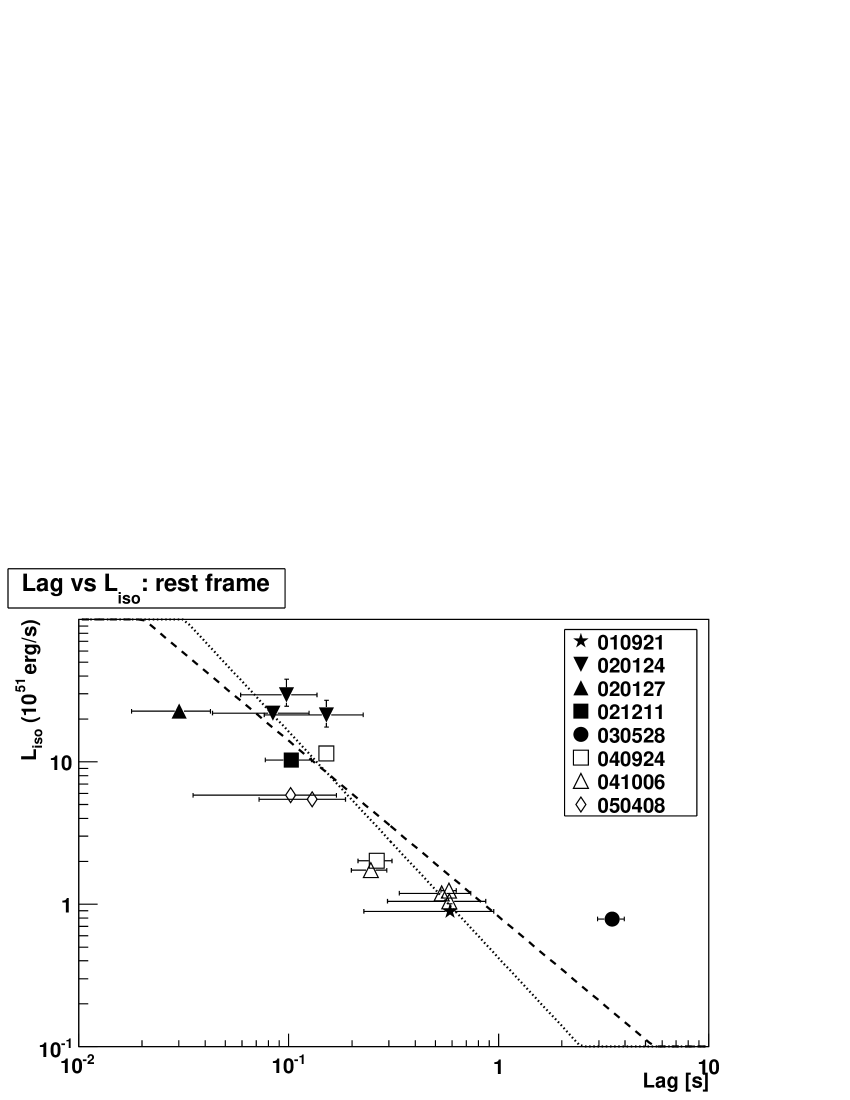
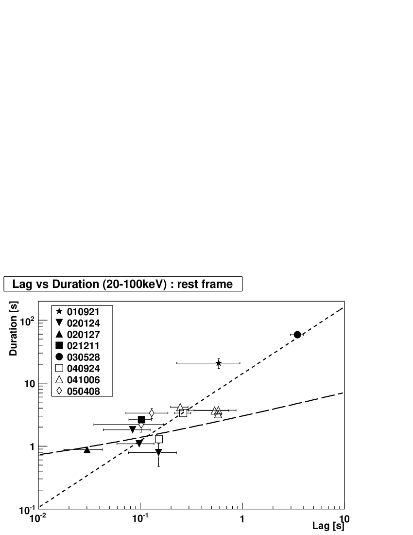
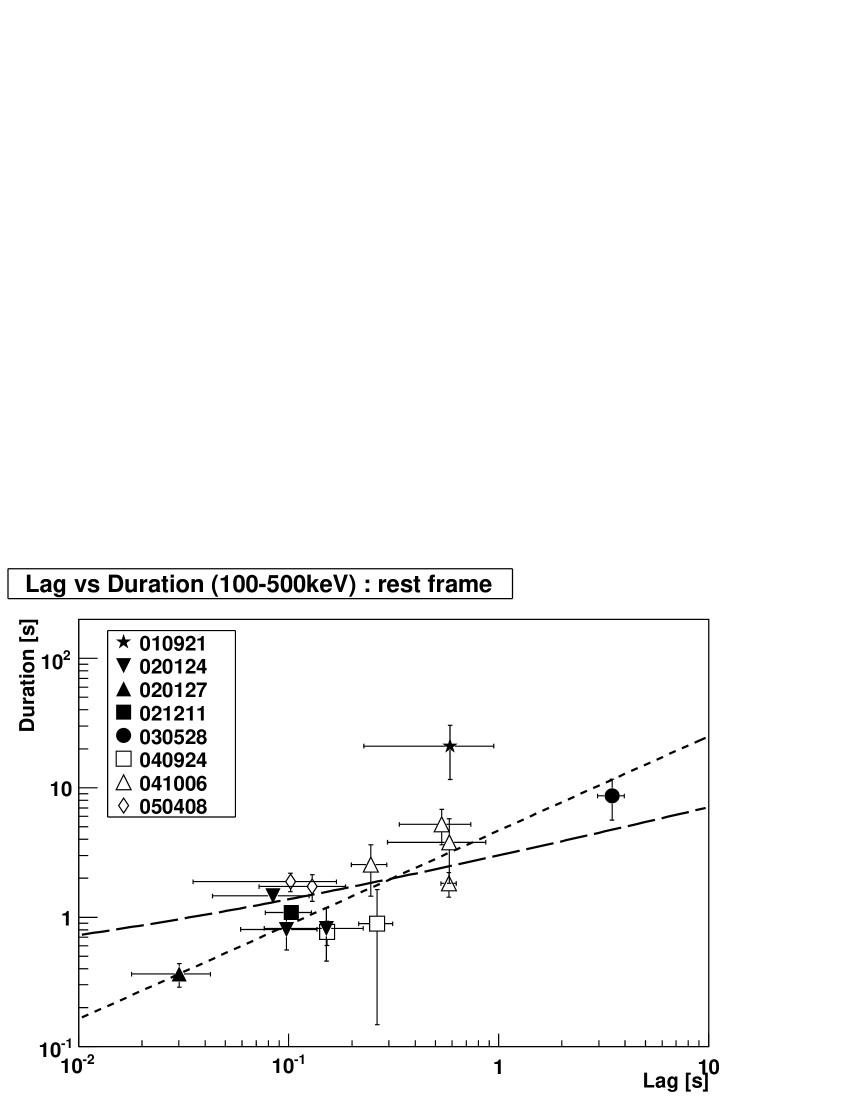
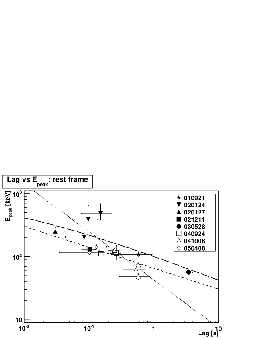
Figure 4: Scatter plots (burst rest frame) of spectral lag vs. luminosity (top left), duration for the low-energy band (top right), duration for the high-energy band (bottom left), and $E_{\rm peak}$ (bottom right). The dashed lines represent the best-fit functions. For the last three plots, the long dashed lines show the theoretical curve expected in the off-axis model (Ioka & Nakamura, 2001). The dotted lines represent the best-fit functions including the systematic uncertainty and excluding GRB 030528.

4.3.2 Yonetoku Relation

We now consider the consistency with the Yonetoku relation (Yonetoku et al., 2004) in this section. In the preceding section, we have found that the off-axis model reproduces the observational results and have not imposed any limitations such as the Yonetoku relation ($L_{\rm iso}\propto E_{\rm peak}^{2}$).

Assuming that the Yonetoku relation is valid, from our result on the lag-luminosity relation ( $L_{\rm iso}\propto\tau_{\rm lag}^{-1.23\pm 0.07}$), the lag-$E_{\rm peak}$ relation is expected to satisfy

$$E_{\rm peak,exp}\propto L_{\rm iso}^{1/2}\propto\tau_{\rm lag}^{-1.23/2}\propto\tau_{\rm lag}^{-0.62}$$ (10)

The index (-0.62) is small compared with the obtained result ($E_{\rm peak,obs}\propto\tau_{\rm lag}^{-0.33\pm 0.03})$. Note that the subscripts “exp” and “obs” represent the expected and observed values, respectively.

Let us assume that the determination of the spectral lag has a systematic uncertainty $\sigma_{\rm sys}$ of 0.05 s resulting from the overlaps of the GRB pulses or some calibration uncertainties. In addition we exclude the peculiar case of GRB 030528, which has a very long spectral lag that may be due to the overlaps of multiple pulses. Then, the best-fit functions become $\log(L_{51})=(-1.38\pm 0.13)-(1.59\pm 0.28)\log(\tau_{\rm lag})$ with reduced chi-square $\chi_{\nu}^{2}$ = 8.2/12, and $\log(E_{\rm peak})=(1.63\pm 0.08)-(0.76\pm 0.17)\log(\tau_{\rm lag})$ with reduced chi-square $\chi_{\nu}^{2}$ = 12.5/12. The Yonetoku relation and the revised lag-luminosity relation give us

$$E_{\rm peak,exp}\propto\tau_{\rm lag}^{-1.59/2}\propto\tau_{\rm lag}^{-0.80},$$ (11)

which agrees with the revised result (index $-0.76$). Therefore, considering the small sample and observational uncertainties, we cannot exclude the validity of the Yonetoku relation from our results.

5 Detailed Energy Dependence of Spectral Lag and Other Properties

Next we consider the detailed energy dependence of the spectral lag and other properties (the durations including the rise and decay times), besides the lag-luminosity relation described in the former sections.

5.1 Energy Dependence of Duration, Rise and Decay Phase

Zhang et al. (2007) studied the energy dependence of temporal properties represented by the formulae,

$$w \propto E^{\alpha_{\rm w}},$$ (12)

$$\tau_{\rm rise} \equiv \frac{1}{2}(w-\tau_{2})\propto E^{\alpha_{\rm rise}},$$ (13)

$$\tau_{\rm decay} \equiv \frac{1}{2}(w+\tau_{2})\propto E^{\alpha_{\rm dec}},$$ (14)

where $\tau_{\rm rise}$ and $\tau_{\rm decay}$ are the rise and decay timescales (Norris et al., 2005). They found that $\alpha_{\rm w}$ and $\alpha_{\rm dec}$ are highly correlated, while $\alpha_{\rm w}$ and $\alpha_{\rm rise}$ are not strongly correlated. Here, it may be reasonable to assume that the intrinsic pulse width is responsible for the rise phase timescale, while the decay phase timescale is determined by the geometrical effect in the relativistic expanding shell. Furthermore, the decay time interval dominates the duration because the typical pulse shape shows a fast rise and exponential decay (FRED). Thus, it is natural that the decay phase is highly dependent on the duration and the rise phase is not strongly related to the duration (or decay time).

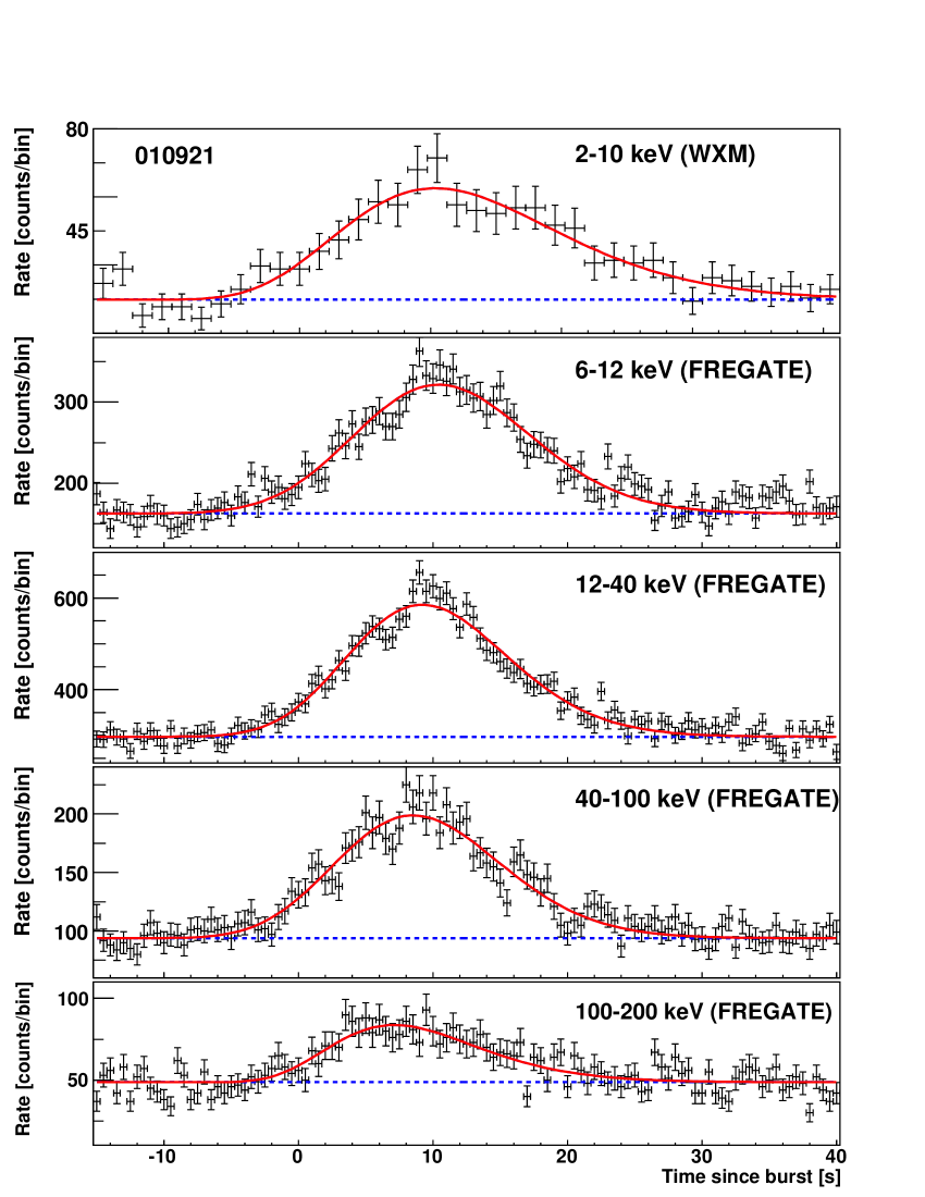
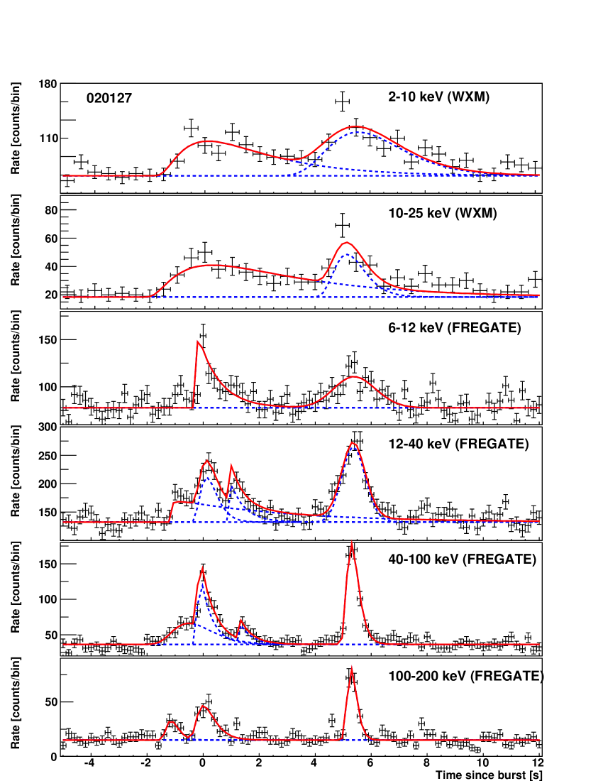
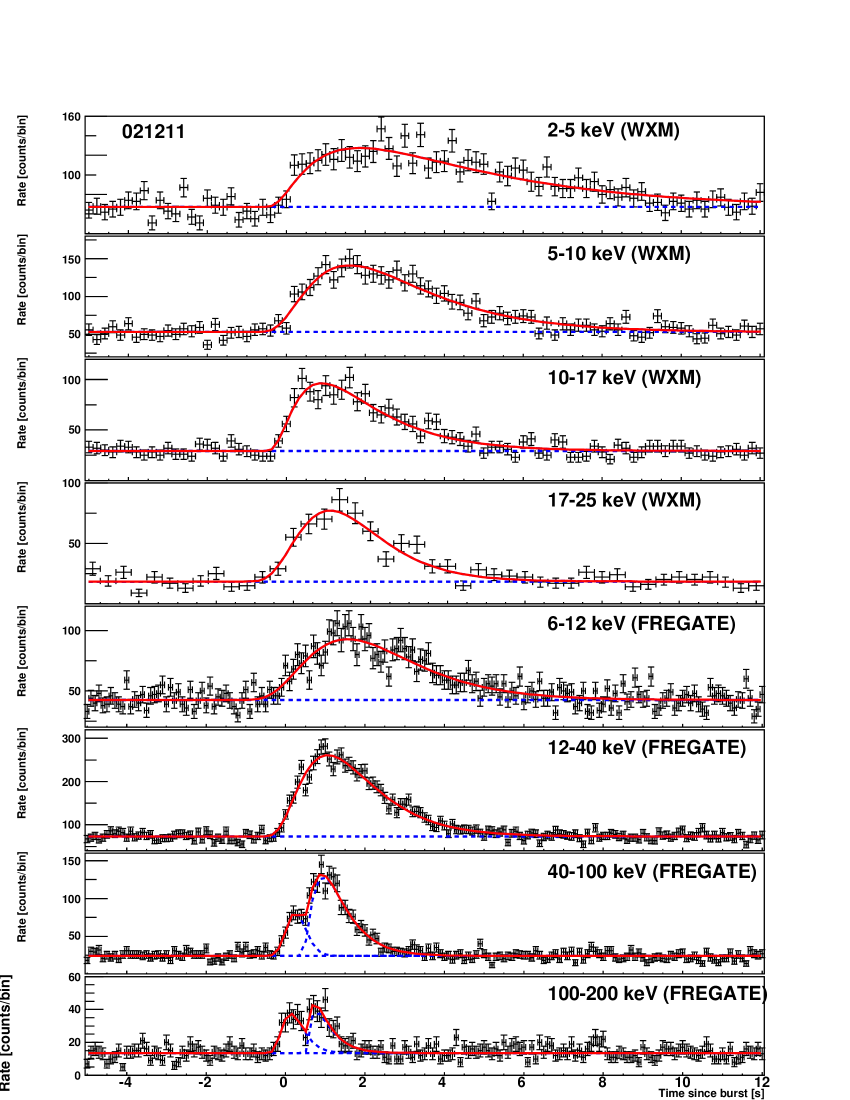
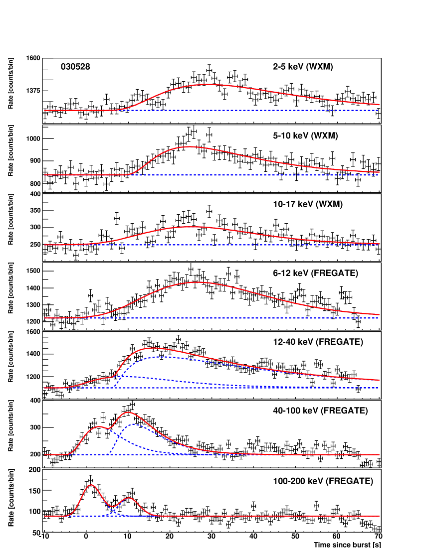
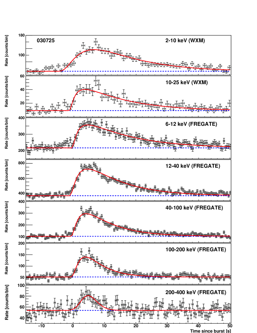
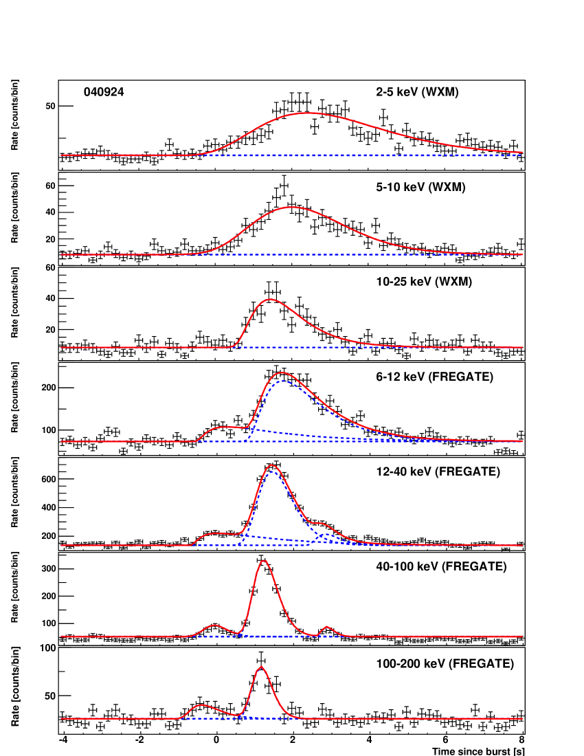
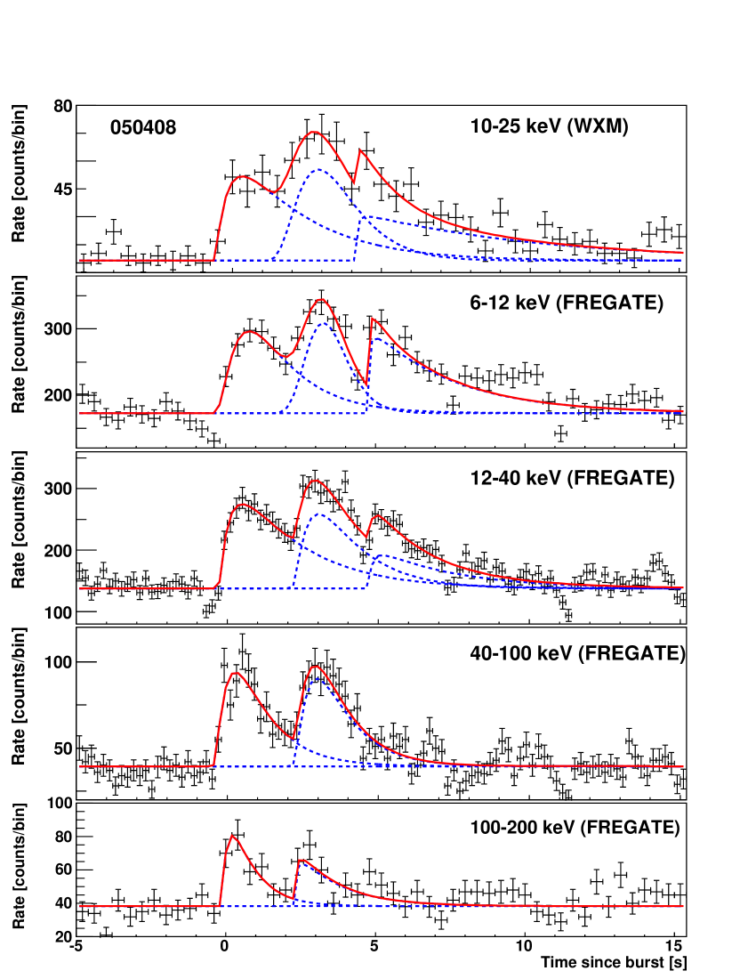
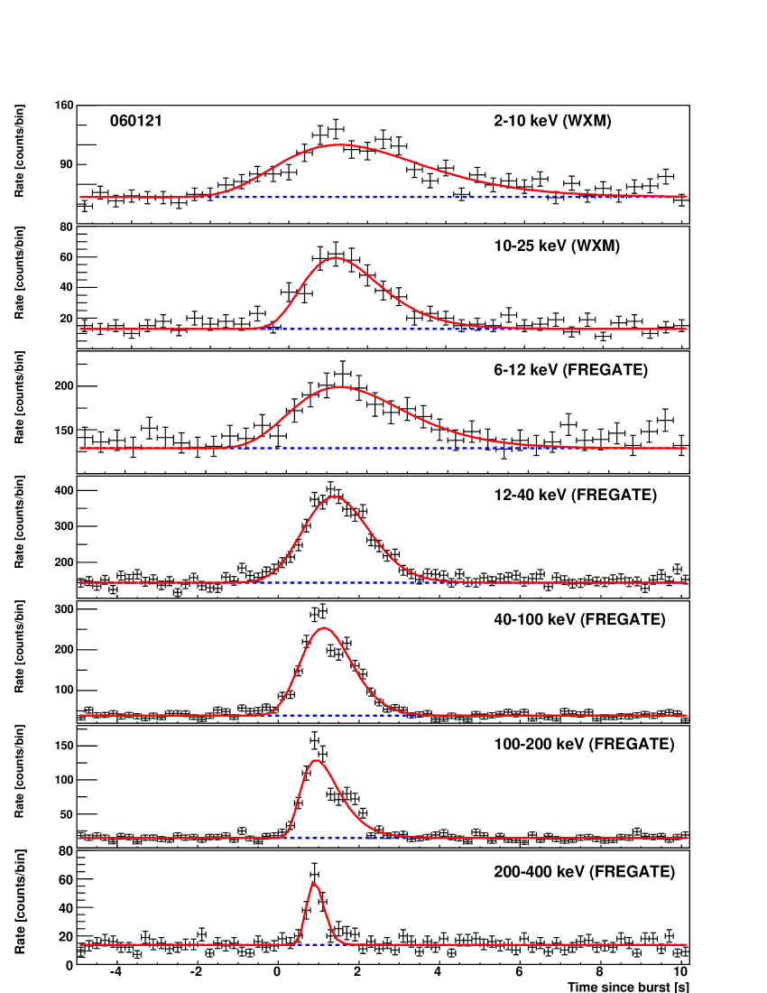
Figure 9: The result of fitted pulses in multiple energy bands.

We show the results of the plots among $\alpha_{\rm w}$, $\alpha_{\rm rise}$ and $\alpha_{\rm dec}$ in Fig. 5 (The result of the fitted pulses is shown in Fig. 9). The top panel of Fig. 5 shows the scatter plot of $\alpha_{\rm w}$ versus $\alpha_{\rm rise}$ in our HETE-2 sample. Although the uncertainty for each point is very large, we find a marginal linear relation with correlation coefficient $R=0.51^{+0.18}_{-0.38}$. The best-fit function is $\alpha_{\rm rise}=(0.04\pm 0.15)+(1.06\pm 0.41)\alpha_{\rm w}$. If the rise timescale is determined only by the intrinsic pulse width, the correlation between $\alpha_{\rm rise}$ and $\alpha_{\rm w}$ should be weak. However, from this result $\alpha_{\rm w}$ seems to be roughly proportional to $\alpha_{\rm rise}$. Therefore, the rise timescale depends not only on the the intrinsic pulse width but also somewhat on the geometrical (curvature) effect. Some previous studies may give us clues to understanding this behavior; Lu et al. (2007) and Peng et al. (2009) found that $E_{\rm peak}$ decays monotonically through long GRB pulses. This energy decay occurs even prior to the pulse peak, namely in the rise time phase. Therefore, the pulse rise phase is a part of the $E_{\rm peak}$-decay phase. Hakkila & Cumbee (2009) also demonstrated that the high-energy pulse intensity is starting to decline prior to the pulse peak in the low-energy band, as is the case for the HETE-2 results. Thus, these results indirectly indicate that the pulse rise timescale is affected by the pulse decay time.

The middle panel of Fig. 5 shows the scatter plot of $\alpha_{\rm w}$ versus $\alpha_{\rm dec}$. The best-fit function is $\alpha_{\rm dec}=(-0.01\pm 0.13)+(1.03\pm 0.37)\alpha_{\rm w}$ with correlation coefficient $R=0.67^{+0.13}_{-0.37}$. Since a relatively good proportionality between $\alpha_{\rm w}$ and $\alpha_{\rm dec}$ exists, this result supports the approximation $w\sim\tau_{\rm decay}$ and the assumption that the curvature effect determines the decay timescale.

The relations between $\alpha_{\rm rise}$ versus $\alpha_{\rm dec}$ are plotted in the bottom panel of Fig. 5, where the best-fit function is $\alpha_{\rm dec}=(-0.04\pm 0.13)+(0.99\pm 0.40)\alpha_{\rm rise}$ with correlation coefficient $R=0.46^{+0.20}_{-0.38}$. The result also seems to show that the rise timescale is slightly affected by the curvature effect. Although the uncertainties in the correlation coefficient and fitting parameters are large, the relationships between $\alpha_{\rm w}$, $\alpha_{\rm rise}$ and $\alpha_{\rm dec}$ are consistent with those of Zhang et al. (2007) (the three functional forms agree with ours).

Shen et al. (2005) computed the temporal profiles of the GRB pulse in the four BATSE energy bands, with the relativistic curvature effect of an expanding shell. They included an intrinsic “Band” shape spectrum and an intrinsic energy-independent emission profile, and estimated the dependence of the duration and other properties on energy as $w$ $\propto$ $E^{-0.2\sim-0.1}$ ($\alpha_{\rm w}\simeq\alpha_{\rm dec}=-0.2$ to $-0.1$). On the other hand, Daigne & Mochkovitch (1998) calculated the time-evolution of the internal shocks (hydrodynamical effect) assuming a highly non-uniform distribution of the Lorentz factor, and obtained the energy dependence as $w\propto$ $E^{-0.4}$.

In our result, shown in Fig. 5, $\alpha_{\rm w}$ and $\alpha_{\rm dec}$ range from -0.8 to 0 and the expected energy dependences for the models of Daigne & Mochkovitch (1998) and Shen et al. (2005) are represented as a long dashed line and a shaded portion, respectively. The data points are widely scattered so that the simple model of Daigne & Mochkovitch (1998) or Shen et al. (2005) alone cannot explain the results we obtained.

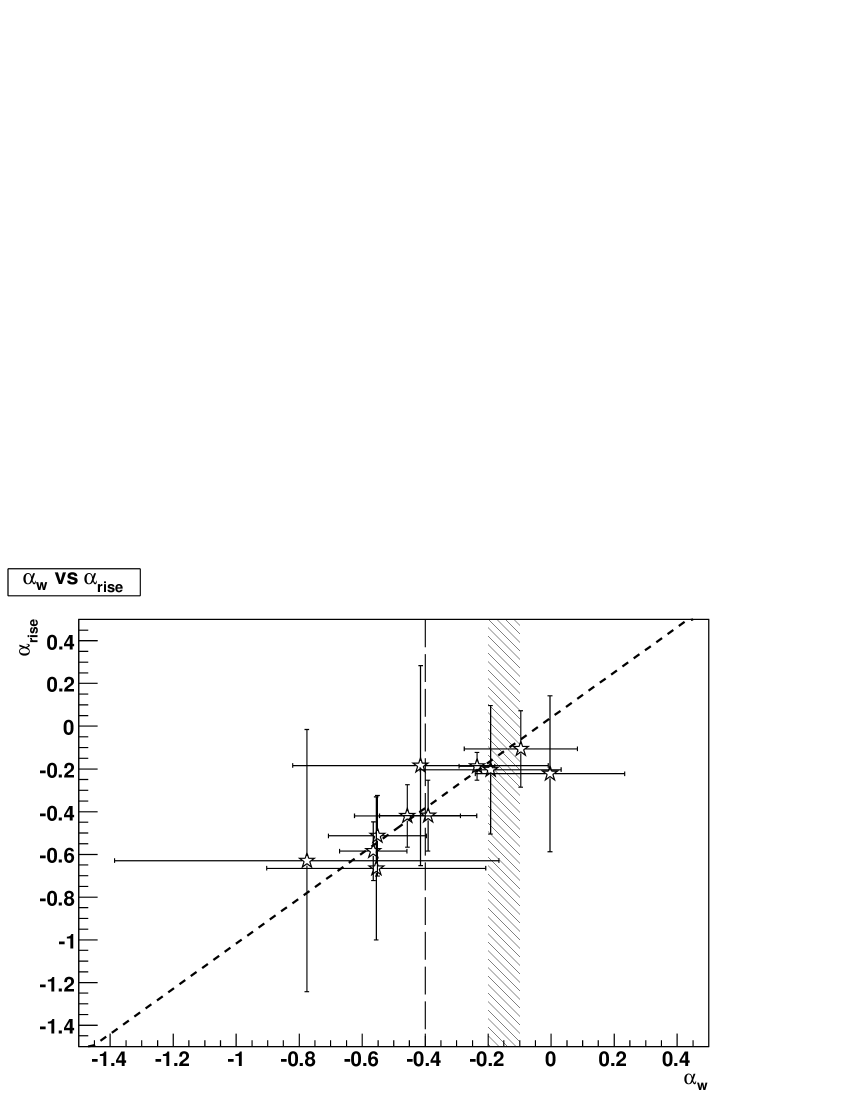
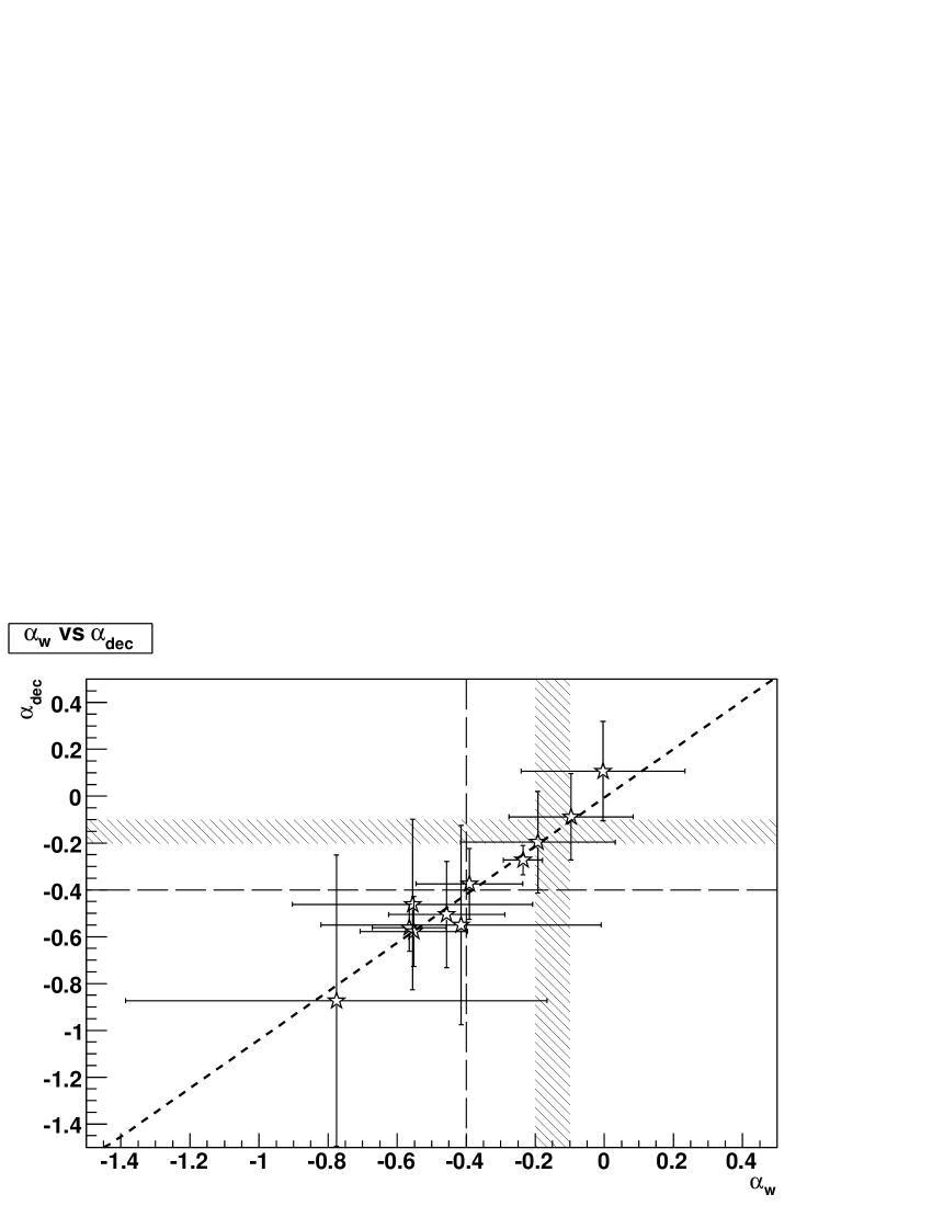
Figure 5: The scatter plots for indices of $\alpha_{\rm w}$, $\alpha_{\rm rise}$ and $\alpha_{\rm dec}$. (Top): $\alpha_{\rm w}$ vs. $\alpha_{\rm rise}$. (Middle): $\alpha_{\rm w}$ vs. $\alpha_{\rm dec}$. (Bottom): $\alpha_{\rm rise}$ vs. $\alpha_{\rm dec}$. The dashed line shows the best-fit linear function. The shaded area and long vertical and horizontal dashed lines represent the expected values from the simple curvature (Shen et al., 2005) and hydrodynamical effects (Daigne & Mochkovitch, 1998), respectively.

5.2 Physical Origin of the Spectral Lag for Individual Pulses

In this section, we try to clarify the origin of the spectral lag of our HETE-2 GRBs, apart from the lag-luminosity relation described in the preceding section. First we need to check whether only the simple curvature effect, which should be in any case included, can explain the energy dependence of the lag or not. Here we consider the curvature effect model described by Lu et al. (2006). They calculated the light curves from an isotropically expanding sphere with a constant bulk Lorentz factor and the Band function for a rest-frame radiation spectrum. A Gaussian pulse was assumed for the light curve in the source rest frame. While the generic formula for the spectral lag is complicated, they demonstrated that the spectral lag has a energy dependence with lag $\propto$ $E$ below a saturated energy, $E_{s}=1.67E_{\rm peak}$ for the typical parameter sets of the low-energy index $\alpha_{B}$ = -1, high-energy index $\beta_{B}$ = -2.25 and the shell radius $r_{0}$ = 3 $\times$ 10¹⁵ cm. Considering the beaming effect, photons of energy at $E>E_{s}$ would mainly come from the area of the surface around the line of sight, i.e., $\theta\lesssim\Gamma^{-1}$ (where $\theta$ is the angle to the line of sight). When $E>E_{s}$, the contribution to the corresponding light curve largely comes from the high-energy portion of the rest frame spectrum, which causes the peak time of the light curve to change less, and the lag would saturate. On the other hand, for $E<E_{\rm s}$, “off-axis” ($\theta>\Gamma^{-1}$) photons may contribute to the light curve so that the lag increases with the increasing energy difference in two energy bands.

We choose the peak time at the lowest energy ($\sim$ 1 keV) arbitrarily to match the observational value of $T_{\rm peak}$. Lu et al. (2006) showed that the lag does not depend strongly on the radius $r_{0}$. So based on their results, we write approximately

$$\tau_{\rm lag}=\left\{\begin{array}[]{ll}aE,&\mbox{if }E\leq E_{s}\\ aE_{s},&\mbox{if }E_{s}<E\\ \end{array}\right.$$ (17)

$$\mbox{where }a=10^{-2.4}\left(\frac{\Gamma}{100}\right)^{-2.8}\mbox{[s/keV]}.$$ (18)

Then $T_{\rm peak}$ is written as

$$T_{\rm peak}=t_{0}-\tau_{\rm lag}=\left\{\begin{array}[]{ll}t_{0}-aE,&\mbox{if }E\leq E_{s}\\ t_{0}-aE_{s},&\mbox{if }E_{s}<E\\ \end{array}\right.$$ (21)

where $t_{0}$ is the peak time at the lowest energy. Using Eq. 21, we try to reproduce the spectral lag for the examined pulses with the curvature effect by adjusting bulk Lorentz factor $\Gamma$ in Fig. 6 and 7. Here, the energy and $T_{\rm peak}$ are translated into the burst rest frame ones with known redshifts, and for GRB 030725 and GRB 060121 without known redshifts assuming that their redshifts are 1. Although our fits are based on an empirical formula with a particular parameter set ($\alpha_{B}$ = -1, $\beta_{B}$ = -2.25), the data points do not largely contradict the tendency predicted by the curvature effect at a particular bulk Lorentz factor $\Gamma$, as shown in Fig. 6. But for some pulses such as GRB 021211, the 2nd pulse of GRB 040924, the 2nd pulse of GRB 050408 and GRB 030725, the model we adopt cannot reproduce the spectral lag well as shown in Fig. 7. Even for such pulses changing the parameters that we have fixed here may soften the contradictions. Alternatively, the off-axis model or the temporal evolution of the internal shock propagation may play an important role in the spectral lag, or a pulse-overlap effect may be included.

To examine whether the pulse duration and spectral lag are explained synthetically by the curvature effect, we summarize the results of the estimated $\Gamma$, $\alpha_{\rm w}$ and other properties in Table 3. The empirical formula based on Lu et al. (2006) has been derived from the assumption for the intrinsic pulse duration $\Delta t_{\rm int}$ = 10⁵ s in the source frame. Although there is no reason to adopt this value, the resultant timescales estimated from the obtained $\Gamma$ are of the same order of magnitude as 10⁵ s. Even for the GRBs whose spectral lag can be explained by the curvature effect, it is hard to confirm the consistency between the prediction of the energy dependence of the pulse duration by the curvature effect ($\alpha_{\rm w}$ = -0.2$\sim$-0.1) and the experimental values because of the large uncertainties in $\alpha_{\rm w}$. However, we may say that the model based on the curvature effect does not contradict both the spectral lag and duration at a particular bulk Lorentz factor $\Gamma$. Thus, the spectral lag can be a tool to help estimate the bulk Lorentz factors.

Since in this analysis only a finite energy range (2$-$400 keV) is available, there are only a small number of points for the energy range, where the lag is saturated above $E_{s}$. For many GRBs, we could only plot one point above $E_{s}$, which leaves the possibility that a significant lag takes place above $E_{s}$ (no saturated energy). Even in the study by Liang et al. (2006), although the peak energy $E_{\rm peak}$ is $\sim$ 54 keV, they also could plot only one point for $T_{\rm peak}$ above $E_{\rm peak}$ due to the poor effective area for the higher energy ranges. To clarify the origin of the spectral lag further, we need to detect GRB photons in the higher energy ranges above $E_{\rm peak}$ to describe the light curve and determine $T_{\rm peak}$ with confidence.

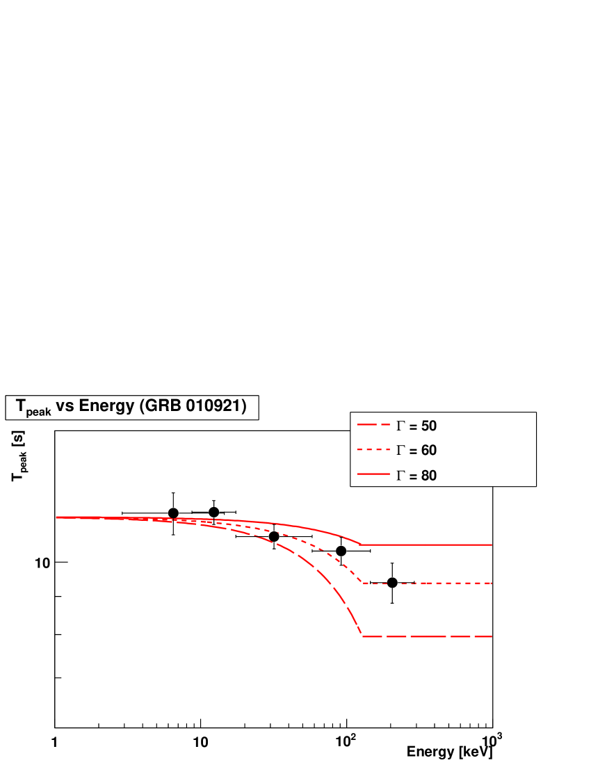
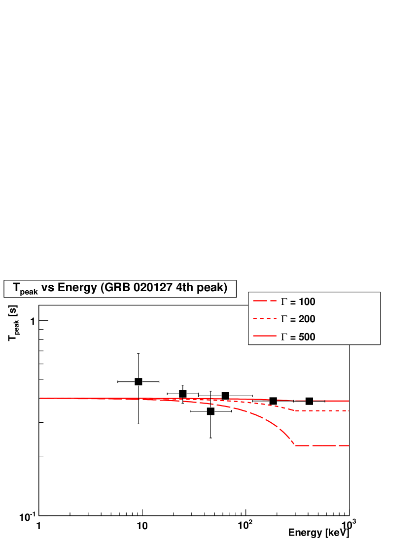
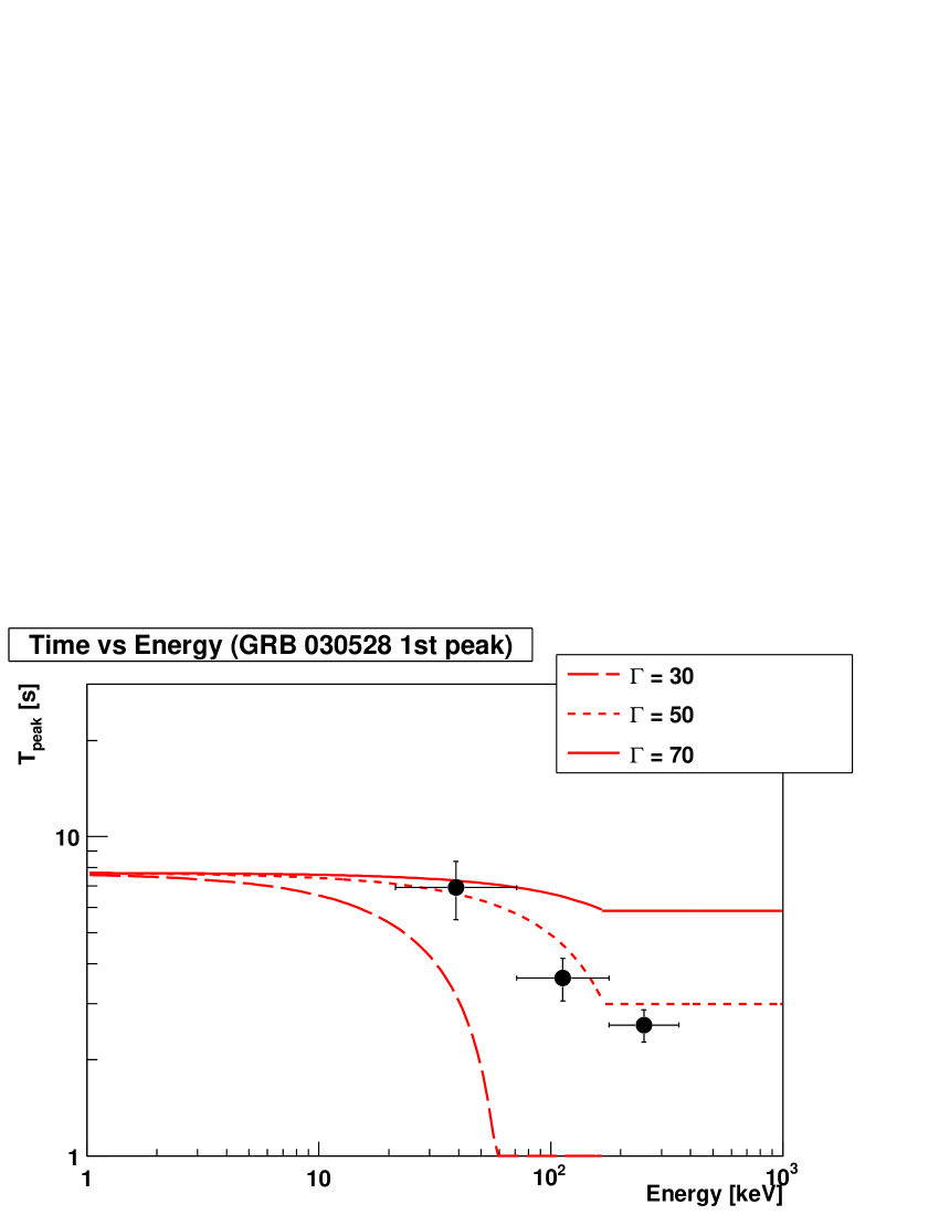
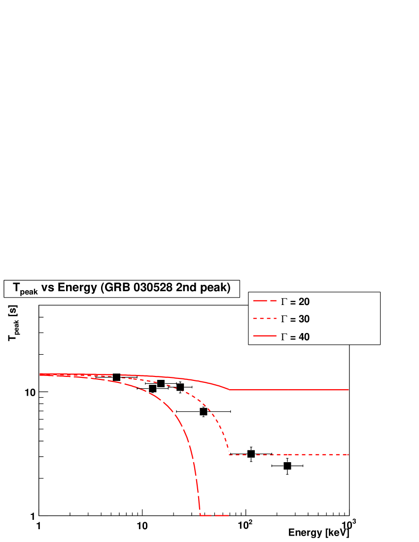
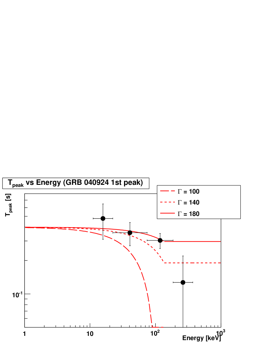
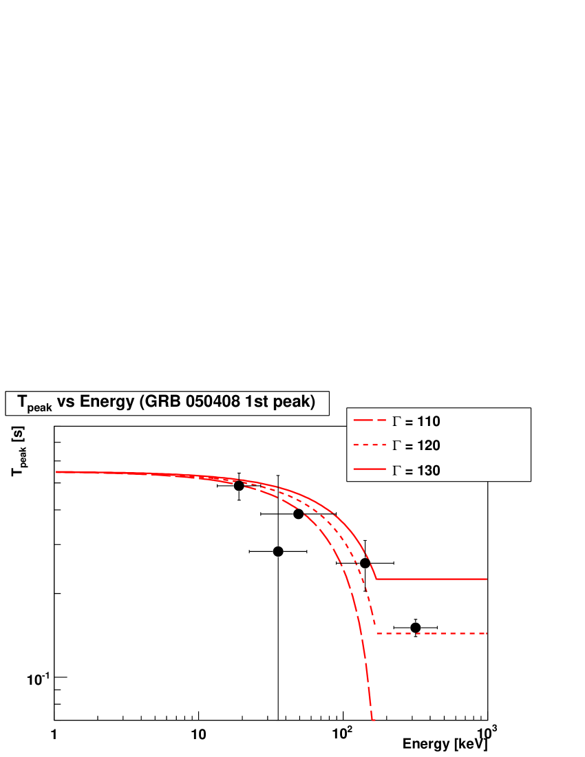
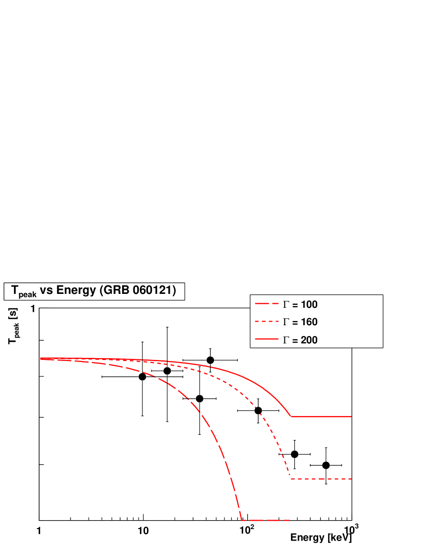
Figure 6: Energy vs. $T_{\rm peak}$ plots in the burst rest frame with the theoretical model lines, showing good agreement with the curvature case. Each line represents the curvature-effect line at the corresponding bulk Lorentz factor $\Gamma$.

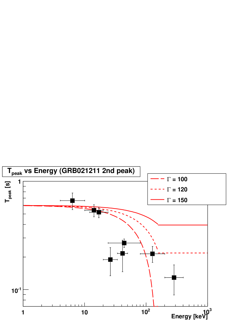
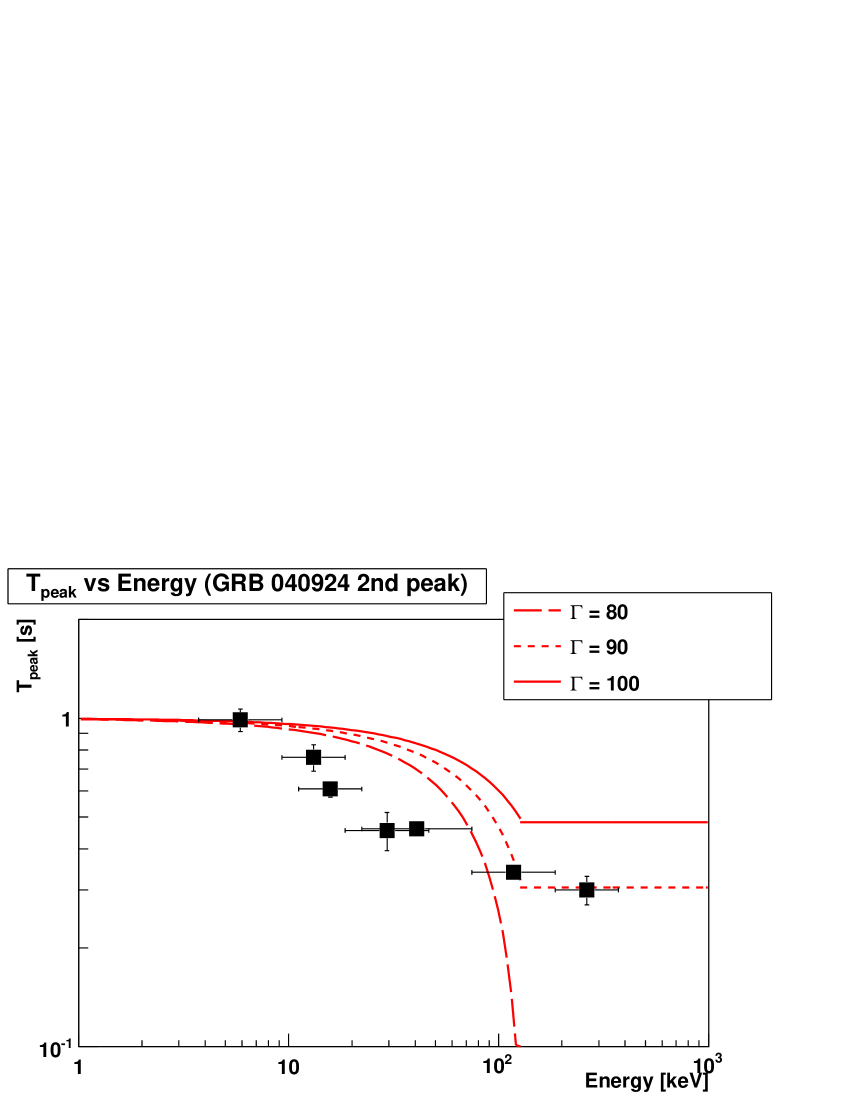
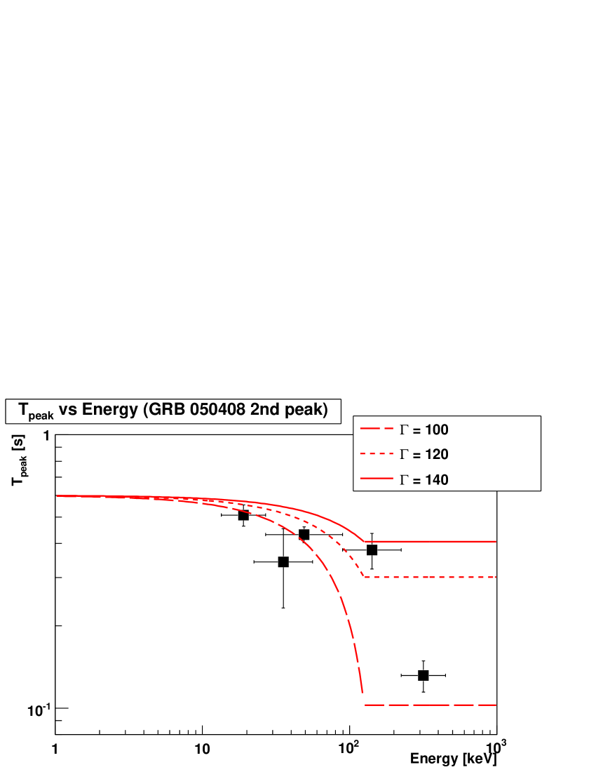
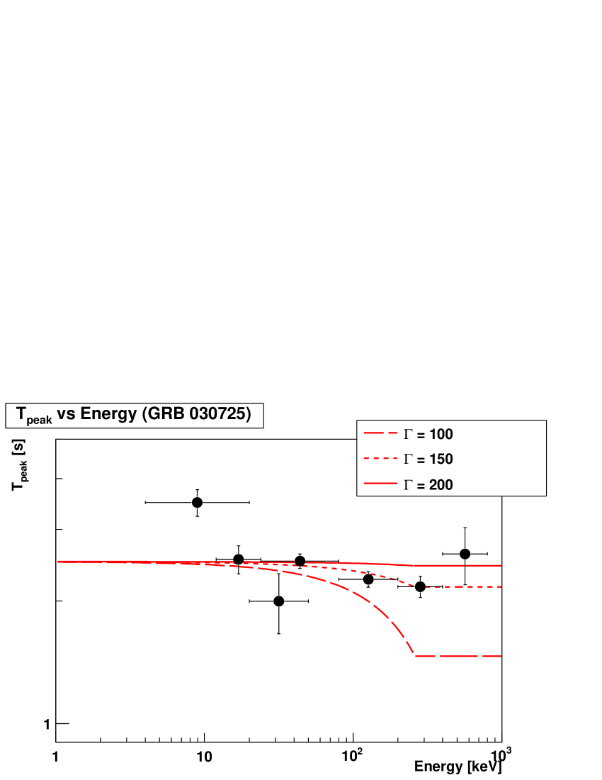
Figure 7: Energy vs. $T_{\rm peak}$ plots in the burst rest frame with the theoretical model lines, showing poor agreement with the curvature case. Each line represents the curvature-effect line at the corresponding bulk Lorentz factor $\Gamma$.

Table 2: Fitting parameters of the lag-luminosity -duration -$E_{\rm peak}$ relations

		$A$	$B$	reduced chi-square	correlation coefficient
luminosity†	obs	-0.79$\pm$0.04	-1.16$\pm$0.07	133.2/12	-0.79${}^{+0.16}_{-0.05}$
	rest	-1.09$\pm$0.04	-1.23$\pm$0.07	97.1/13	-0.90${}^{+0.12}_{-0.02}$
duration⋄	obs	1.05$\pm$0.06	1.16$\pm$0.09	43.0/12	0.66${}^{+0.10}_{-0.14}$
(low energy)	rest	1.06$\pm$0.04	1.15$\pm$0.06	72.5/13	0.74${}^{+0.06}_{-0.15}$
duration⋄	obs	0.69$\pm$0.05	0.94$\pm$0.08	45.1/12	0.74${}^{+0.06}_{-0.14}$
(high energy)	rest	0.67$\pm$0.06	0.73$\pm$0.09	26.6/13	0.72${}^{+0.07}_{-0.22}$
$E_{\rm peak}$∗	obs	1.88$\pm$0.02	-0.31$\pm$0.02	97.8/12	-0.66${}^{+0.15}_{-0.08}$
	rest	1.82$\pm$0.02	-0.33$\pm$0.03	33.9/13	-0.81${}^{+0.16}_{-0.05}$
†: $\log(L_{51})$ = $A+B\log(\tau_{\rm lag})$, ⋄: $\log(\omega)$ = $A+B\log(\tau_{\rm lag})$, ∗: $\log(E_{\rm peak})$ = $A+B\log(\tau_{\rm lag})$
Note that ”obs” represents the observer’s frame and ”rest” represents the rest frame.

Table 3: Summary of the obtained bulk Lorentz factor, the power-law index of the duration, the observed duration and the expected intrinsic pulse width

GRB	$\Gamma$	$\alpha_{\rm w}$	$w_{\rm obs}$ [s]	$\Delta t^{\rm exp}_{\rm int}$ [s]
010921	60	-0.11$\pm$0.18	21.4$\pm$2.9	0.77$\times$105
020127	500	-0.67$\pm$0.34	0.70$\pm$0.01	1.75$\times$105
030528 (1st pulse)	50	-0.63$\pm$0.61	26.1$\pm$14.7	0.65$\times$105
030528 (2nd pulse)	30	-0.42$\pm$0.15	58.8$\pm$6.8	0.53$\times$105
040924 (1st pulse)	140	-0.18$\pm$0.47	1.8$\pm$0.5	0.35$\times$105
050408 (1st pulse)	120	-0.20$\pm$0.30	2.8$\pm$0.2	0.40$\times$105
060121	160	-0.42$\pm$0.17	1.8$\pm$0.2	0.46$\times$105
021211	-	-0.58$\pm$0.14	2.4$\pm$0.1	-
030725	-	-0.18$\pm$0.07	19.7$\pm$0.5	-
040924 (2nd pulse)	-	-0.51$\pm$0.19	1.4$\pm$0.1	-
050408 (2nd pulse)	-	-0.22$\pm$0.36	2.0$\pm$0.2	-

Note that the bulk Lorentz factor $\Gamma$ is estimated by the lag analysis in Fig. 6 and $w_{\rm obs}$ is the observed duration in the burst rest frame and $\Delta t^{\rm exp}_{\rm int}$ is the expected intrinsic pulse width from the obtained bulk Lorentz factor $\Gamma$.

6 Towards a Unified Theory

Our results suggest that there are correlations between the spectral lag and other observational properties for each GRB pulse. The correlations we found and some additional pulse correlations such as spectral hardness or pulse asymmetry etc. reported by Hakkila & Cumbee (2009) are important hints to specify or constrain models of GRB prompt emission.

On the other hand, because of the large dispersions, the spectral lag relations are not so useful as tools to measure cosmological distances so far, compared with the Yonetoku relation. We should note that there may still be systematic uncertainties in the obtained lags, which may change the correlations as discussed in §4.3.2. While the obtained lag-luminosity, -$E_{\rm peak}$ and -duration relations can be consistent with a specific model, namely the off-axis model suggested by Ioka & Nakamura (2001), the energy dependences of the spectral lag seem to be consistent with the simple curvature effects for some GRB pulses. The assumptions inferred in Ioka & Nakamura (2001) and Lu et al. (2006) are different so that we have discussed the correlations and energy-dependences in the spectral lag with two independent models. Although such methods do not give us a consistent picture for the spectral lag so far, the discussion in this paper may help to determine which models are more appropriate.

For a unified theory to explain the spectral lag and other temporal spectral characteristics, the effect of the curvature, viewing with an offset angle to the jet, time-evolution of shock propagation, and other effects must be taken into account synthetically and theoretical investigations need to be done. To have further quantitative discussions, we need a sample which includes many GRBs having a good S/N ratio detected in a wide band (keV$-$GeV) with observationally known redshifts.

We appreciate the referee, Prof. Jon Hakkila, for his fruitful comments, which have improved our paper. M. A. acknowledges the financial support from the Global Center of Excellence Program by MEXT, Japan through the Nanoscience and Quantum Physics Project of the Tokyo Institute of Technology. This work has been supported by Japanese Grant-in-Aid for Young Scientists (B) 20740102. G. P. acknowledges financial support a part of ASI contract I/088/06/0.

References

- Band et al. (1993) Band, D., et al. 1993, ApJ, 413, 281
- Berger et al. (2005) Berger, E., Gladders, M., & Oemler, G. 2005, GRB Coordinates Network, 3201, 1
- Berger et al. (2007) Berger, E., Fox, D. B., Kulkarni, S. R., Frail, D. A., & Djorgovski, S. G. 2007, ApJ, 660, 504
- Bošnjak et al. (2009) Bošnjak, Ž., Daigne, F., & Dubus, G. 2009, A&A, 498, 677
- Daigne & Mochkovitch (1998) Daigne, F., & Mochkovitch, R. 1998, MNRAS, 296, 275
- Daigne & Mochkovitch (2003) Daigne, F., & Mochkovitch, R. 2003, MNRAS, 342, 587
- de Ugarte Postigo et al. (2006) de Ugarte Postigo, A., et al. 2006, ApJ, 648, L83
- Djorgovski et al. (2001) Djorgovski S. G. et al., 2001, GRB Coordinates Network, 1108, 1
- Hakkila et al. (2008) Hakkila, J., Giblin, T. W., Norris, J. P., Fragile, P. C., & Bonnell, J. T. 2008, ApJ, 677, L81
- Hakkila & Cumbee (2009) Hakkila, J., & Cumbee, R. S. 2009, American Institute of Physics Conference Series, 1133, 379
- Hakkila & Nemiroff (2009) Hakkila, J., & Nemiroff, R. J. 2009, ApJ, 705, 372
- Hjorth et al. (2003) Hjorth, J., et al. 2003, ApJ, 597, 699
- Ioka & Nakamura (2001) Ioka, K., & Nakamura, T. 2001, ApJ, 554, L163
- Liang et al. (2006) Liang, E.-W., Zhang, B.-B., Stamatikos, M., Zhang, B., Norris, J., Gehrels, N., Zhang, J., & Dai, Z. G. 2006, ApJ, 653, L81
- Lu et al. (2006) Lu, R.-J., Qin, Y.-P., Zhang, Z.-B., & Yi, T.-F. 2006, MNRAS, 367, 275
- Lu et al. (2007) Lu, R.-J., Peng, Z.-Y., & Dong, W. 2007, ApJ, 663, 1110
- Norris et al. (2000) Norris, J. P., Marani, G. F., & Bonnell, J. T. 2000, ApJ, 534, 248
- Norris et al. (2005) Norris, J. P., Bonnell, J. T., Kazanas, D., Scargle, J. D., Hakkila, J., & Giblin, T. W. 2005, ApJ, 627, 324
- Peng et al. (2009) Peng, Z. Y., Ma, L., Zhao, X. H., Yin, Y., Fang, L. M., & Bao, Y. Y. 2009, ApJ, 698, 417
- Pugliese et al. (2005) Pugliese, G., et al. 2005, A&A, 439, 527
- Qin (2002) Qin, Y.-P. 2002, A&A, 396, 705
- Qin et al. (2004) Qin, Y.-P., Zhang, Z.-B., Zhang, F.-W., & Cui, X.-H. 2004, ApJ, 617, 439
- Qin & Lu, (2005) Qin, Y.-P., & Lu, R.-J. 2005, MNRAS, 362, 1085
- Rau et al. (2005) Rau, A., Salvato, M., & Greiner, J. 2005, A&A, 444, 425
- Shen et al. (2005) Shen, R.-F. , Song, L.-M., & Li, Z. 2005, MNRAS, 362, 59
- Stanek et al. (2005) Stanek, K. Z., et al. 2005, ApJ, 626, L5
- Yonetoku et al. (2004) Yonetoku, D., Murakami, T., Nakamura, T., Yamazaki, R., Inoue, A. K., & Ioka, K. 2004, ApJ, 609, 935
- Vreeswijk et al. (2003) Vreeswijk, P., Fruchter, A., Hjorth, J., & Kouveliotou, C. 2003, GRB Coordinates Network, 1785, 1
- Wiersema et al. (2004) Wiersema, K., Starling, R. L. C., Rol, E., Vreeswijk, P., & Wijers, R. A. M. J. 2004, GRB Coordinates Network, 2800, 1
- Zhang et al. (2007) Zhang, F.-W., Qin, Y.-P., & Zhang, B.-B. 2007, PASJ, 59, 857