Ground state energy of the interacting Bose gas
in two dimensions: an explicit construction

Abstract

The isotropic scattering phase shift is calculated for non-relativistic bosons interacting at low energies via an arbitrary finite-range potential in $d$ spacetime dimensions. Scattering on a $(d-1)$-dimensional torus is then considered, and the eigenvalue equation relating the energy levels on the torus to the scattering phase shift is derived. With this technology in hand, and focusing on the case of two spatial dimensions, a perturbative expansion is developed for the ground-state energy of ${\bf N}$ identical bosons which interact via an arbitrary finite-range potential in a finite area. The leading non-universal effects due to range corrections and three-body forces are included. It is then shown that the thermodynamic limit of the ground-state energy in a finite area can be taken in closed form to obtain the energy-per-particle in the low-density expansion, by explicitly summing the parts of the finite-area energy that diverge with powers of ${\bf N}$. The leading and subleading finite-size corrections to the thermodynamic limit equation-of-state are also computed. Closed-form results –some well-known, others perhaps not– for two-dimensional lattice sums are included in an appendix.

I Introduction

The study of quantum mechanical scattering in a confined geometry is topical in several distinct ways. Recently developed experimental techniques involving trapped ultracold atoms are able to alter spatial dimensionality Hadz ; clade ; posa ; Bloch:2008zz , thus motivating an understanding of the quantum mechanical interactions among atoms as the number of spatial dimensions are continuously varied. Bose gases in two spatial dimensions are of particular interest as they are expected to have a complex phase structure which is quite distinct from their counterparts in three spatial dimensions Mermin:1966fe ; Hohenberg:1967zz ; Kosterlitz:1973xp ; fishe . On the other hand, from the perspective of numerical simulation, scattering in a confined geometry is often a practical necessity. For instance, in lattice studies of quantum field theories, calculations are done in a four-dimensional Euclidean space time volume. For reasons of cost, the finite spatial and temporal extent of these volumes is currently not enormous as compared to the physical length scales that are characteristic of the particles and interactions that are simulated. Moreover, there are no-go theorems Maiani:ca for Euclidean quantum field theory that require a finite volume in order to extract information about hadronic interactions away from kinematic thresholds. The technology required to relate hadronic interactions to the finite-volume singularities that are measured on the lattice has been developed in Refs. Luscher:1986pf ; Luscher:1990ux ; Beane:2003da ; Beane:2007qr ; Tan:2007bg ; Detmold:2008gh and state-of-the-art Lattice QCD calculations have now measured the energy levels of up to twelve interacting pions and allowed a determination of the three-pion interaction Beane:2007es . Similarly, quantum Monte Carlo studies of many-body systems in nuclear and condensed matter physics are carried out in a finite volume or a finite area, and thus a detailed understanding of how the energy levels in the confined geometry map onto continuum physics is essential to controlled predictive power.

The purpose of the present study is several-fold. First, we aim to present a general study of the ground-state energy of a system of ${\bf N}$ bosons interacting via the most general finite-range potential, confined to a finite area. This energy admits a perturbative expansion in the two-body coupling strength for the case of a weak repulsive interaction. As a necessary prelude to considering a confined geometry, we first review the subject of isotropic scattering of identical bosons in $d$ spacetime dimensions using effective field theory (EFT). It is assumed that the reader is aware of the advantages of EFT technology. We then present a general study of the relation between eigenenergies on a torus and continuum-limit isotropic scattering parameters, for any spacetime dimension. While the eigenvalue equation that we obtain is derived in the non-relativistic EFT, it is expected to be generally valid in an arbitrary quantum field theory up to corrections that are exponentially suppressed in the size of the geometric boundary. A general study along these lines in quantum field theory is quite involved and has been carried out only in four spacetime dimensions Luscher:1990ux . The results of that study demonstrated that boundary effects due to polarization are suppressed exponentially with spatial size and therefore the leading power law behavior can be found directly in the non-relativistic theory. Hence the leading effects are captured by the non-relativistic EFT, with relativistic effects appearing perturbatively Beane:2007qr ; Detmold:2008gh . In the case of two spatial dimensions, the exact two-body eigenvalue equation has been considered previously in the context of lattice QED simulations in three spacetime dimensions Fiebig:1994qi . However, there is little discussion in the literature about the consequences of scale invariance in the confined geometry, and about the ground-state energy of the many-body system in a finite area. Moreover, to our knowledge, the closed-form results that exist for the relevant lattice sums in even spatial dimensions, which render this case a particularly interesting theoretical playground, have not been noted previously.

Following our derivation of the ground-state energy of a system of ${\bf N}$ bosons confined to a finite area, we demonstrate that the thermodynamic limit of this system may be taken explicitly, by summing the parts of the expansion that diverge in the large ${\bf N}$ limit. In the thermodynamic limit, the energy-per-particle admits a double perturbative expansion in the two-body coupling and the density. As a byproduct of taking the thermodynamic limit, we are able to compute finite-size corrections to the thermodynamic-limit formula. In addition, we trivially include the leading non-universal corrections due to three-body forces. Study of the weakly interacting Bose gas at zero temperature has a long history, beginning with the mean-field result of Schick schic , with subleading corrections computed in Refs popo ; fishe ; chern ; Andersen . There are some claims in the literature regarding discrepancies among the various studies. We will comment on these claims below.

This paper is organized as follows. In section II we review low-energy non-relativistic scattering of bosons in the continuum. Using EFT we calculate the isotropic phase shift in an arbitrary number of spacetime dimensions. Section III considers low-energy non-relativistic scattering of bosons in a confined geometry, in particular on a $d-1$-dimensional torus. We obtain the exact eigenvalue equation which relates the energy levels on the torus to the two-body continuum-limit scattering parameters. In section IV we consider the ground-state energy of a system of Bosons confined to a finite area. We first develop perturbation theory on the $d-1$-dimensional torus and recover the perturbative expansions of the two-body results found previously. We then focus on ${\bf N}$ bosons interacting via weak repulsive interactions in a finite area and give a general expression for the ground-state energy. In section V we demonstrate how to take the thermodynamic limit in order to recover the well-known low-density expansion, and we compare our results with other calculations. We also compute the leading and subleading finite-size corrections to the thermodynamic-limit energy density. Finally, in section VI we conclude. In two Appendices, we make use of some well-known exact results for even-dimensional lattice sums to derive some closed-form expressions that are useful for the case of two spatial dimensions, and we evaluate several sums involving the Catalan numbers, which are relevant for deriving the thermodynamic-limit equation-of-state.

II Scattering in the continuum

II.1 Generalities

Here we will review some basic EFT technology which will allow us to obtain a general expression for the isotropic scattering phase shift in any number of dimensions. If one is interested in low-energy scattering, an arbitrary interaction potential of finite range may be replaced by an infinite tower of contact operators, with coefficients to be determined either by matching to the full theory or by experiment. At low energies only a few of the contact operators will be important. The EFT of bosons , destroyed by the field operator $\psi$, which interact through contact interactions, has the following Lagrangian:

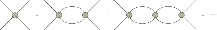
Figure 1: Feynman diagrams that give the exact two-body scattering amplitude. The oval blob represents the all-orders interaction derived from the Lagrangian.

$${\cal L}={{\psi}^{\dagger}}\left(i\partial_{t}+\frac{\nabla^{2}}{2M}\right)\psi-\frac{C_{0}}{4}({{\psi}^{\dagger}}\psi)^{2}-\frac{C_{2}}{8}\nabla({{\psi}^{\dagger}}\psi)\nabla({{\psi}^{\dagger}}\psi)-\frac{D_{0}}{36}({{\psi}^{\dagger}}\psi)^{3}\ +\ \ldots$$ (1)

This Lagrangian, constrained by Galilean invariance, parity and time-reversal invariance, describes Bosons interacting at low-energies via an arbitrary finite-range potential. In principle, it is valid in any number of spacetime dimensions, $d$. The mass dimensions of the boson field and of the operator coefficients change with spacetime dimensions: i.e. $[\psi]=(d-1)/2$, $[C_{2n}]=2-d-2n$ and $[D_{0}]=3-2d$. While our focus in this paper is on $d=3$, in our general discussion of two- and three-body interactions, we will keep $d$ arbitrary as this will allow the reader to check our results against the well-known cases with $d=2$ and $d=4$. Throughout we use units with $\hbar=1$, however we will keep the boson mass, $M$, explicit.

Consider $2\rightarrow 2$ scattering, with incoming momenta labeled ${\bf p}_{1},{\bf p}_{2}$ and outgoing momenta labeled ${\bf p}^{\prime}_{1},{\bf p}^{\prime}_{2}$. In the center-of-mass frame, ${\bf p}={\bf p}_{1}=-{\bf p}_{2}$ , and the sum of Feynman diagrams, shown in fig. 1, computed in the EFT gives the two-body scattering amplitude Braaten:2000eh ; Kaplan:1998we ; vanKolck:1998bw

$${\cal A}_{2}(p) = -{\sum C_{2n}\ p^{2n}\over 1-I_{0}(p)\sum C_{2n}\ p^{2n}}\ ,$$ (2)

where

$$I_{0}(p)\ =\ \frac{M}{2}\left({\mu\over 2}\right)^{\epsilon}\int{d^{D-1}{\bf q}\over(2\pi)^{D-1}}{1\over p^{2}-{{\bf q}^{2}}+i\delta}\ ,$$ (3)

and it is understood that the ultraviolet divergences in the EFT are regulated using dimensional regularization (DR). In eq. (3), $\mu$ and $D$ are the DR scale and dimensionality, respectively, and $\epsilon\equiv d-D$. A useful integral is:

$$\openup 9.0ptI_{n}(p) = \frac{M}{2}\left({\mu\over 2}\right)^{\epsilon}\int{{{\rm d}}^{D-1}{\bf q}\over(2\pi)^{D-1}}\,{\bf q}^{2n}\left({1\over p^{2}-{\bf q}^{2}+i\delta}\right)\ ;$$ (4)

$$= -\frac{M}{2}p^{2n}(-p^{2}-i\delta)^{(D-3)/2}\Gamma\left({3-D\over 2}\right){(\mu/2)^{\epsilon}\over(4\pi)^{(D-1)/2}}\ .$$

In what follows we will define the EFT coefficients in DR with $\overline{MS}$. This choice is by no means generally appropriate Kaplan:1998we ; vanKolck:1998bw . However it is a convenient choice if no assumption is made about the relative size of the renormalized EFT coefficients.

Now we should relate the scattering amplitude in the EFT, $A_{2}(p)$, whose normalization is conventional and fixed to the Feynman diagram expansion, to the S-matrix. We will simply assume that the S-matrix element for isotropic (s-wave) scattering exists in an arbitrary number of spacetime dimensions. We then have generally

$$e^{2i\delta(p)}\ =\ 1\ +\ i\;{\cal N}(p)\;A_{2}(p)\ ,$$ (5)

where ${\cal N}(p)$ is a normalization factor that depends on $d$ and is fixed by unitarity. Indeed combining eq. (2) and eq. (5) gives ${\cal N}(p)=-2{\rm Im}(I_{0}(p))$ and one can parametrize the scattering amplitude by

$${\cal A}_{2}(p)\ =\ \frac{-1}{{\rm Im}(I_{0}(p))\big{[}\cot\delta(p)-i\big{]}}\ ,$$ (6)

with

$$\cot\delta(p)\ =\ \frac{1}{{\rm Im}(I_{0}(p))}\Bigg{[}\frac{1}{\sum C_{2n}\ p^{2n}}\ -\ {\rm Re}(I_{0}(p))\Bigg{]}\ .$$ (7)

Bound states are present if there are poles on the positive imaginary momentum axis. That is if $\cot\delta(i\gamma)=i$ with binding momentum $\gamma>0$. These expressions are valid for any $d$. In order to evaluate $I_{0}(p)$ it is convenient to consider even and odd spacetime dimensions separately. For $d$ even the Gamma function has no poles and one finds

$$I_{0}(p) = -\frac{M}{2(4\pi)^{(d-1)/2}}\frac{\pi i\;p^{d-3}}{\Gamma\left({d-1\over 2}\right)}\ .$$ (8)

As there is no divergence, the $\overline{MS}$ EFT coefficients do not run with $\mu$ in even spacetime dimensions. Hence the bare parameters are the renormalized parameters. For $d$ odd, one finds

$$I_{0}(p)=\frac{M}{2(4\pi)^{(d-1)/2}}\frac{p^{d-3}}{\Gamma\left({d-1\over 2}\right)}\Bigg{[}\log{\left(-\frac{p^{2}}{\mu^{2}}\right)}\ -\ \psi_{0}\left({d-1\over 2}\right)\ -\log\pi\ -\ \frac{2}{\epsilon}\Bigg{]}\ ,$$ (9)

where $\psi_{0}(n)$ is the digamma function. Here there is a single logarithmic divergence, hidden in the $1/\epsilon$ pole. Hence in our scheme, at least one EFT coefficient runs with the scale $\mu$. With these results in hand it is now straightforward to give the general expression for the isotropic phase shift in $d$ spacetime dimensions:

$$p^{d-3}\cot\delta(p)\ =\ -\frac{(4\pi)^{(d-1)/2}}{\pi M}\Gamma\left({d-1\over 2}\right)\frac{2}{\sum C_{2n}\ p^{2n}}\ +\ (1-(-1)^{d})\frac{p^{d-3}}{2\pi}\log{\left(\frac{p^{2}}{\overline{\mu}^{2}}\right)}\ ,$$ (10)

where $\overline{\mu}$ is defined by equating the logarithm in eq. (10) with the content of the square brackets in eq. (9). Note that this is an unrenormalized equation; the $C_{2n}$ coefficients are bare parameters and there is a logarithmic divergence for odd spacetime dimensions. One must expand the right hand side of this equation for small momenta in order to renormalize . It is noteworthy that the effective field theory seems not to exist for $d>3$ and odd as the divergence is generated at leading order and yet requires a nominally suppressed operator for renormalization.

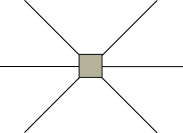
Figure 2: Feynman diagram that gives the leading contribution to the three-body scattering amplitude.

The leading three-body diagram in the momentum expansion is shown in fig. 2, and the three-body scattering amplitude is given by

$${\cal A}_{3}\ =\ -\ D_{0}\ .$$ (12)

II.2 Two spatial dimensions

In this section we consider the case $d=3$ in some detail. This case is particularly interesting because of its analogy with renormalizable quantum field theories, and QCD in particular Kaplan:2005es ; Jackiw:1991je . From our general formula, eq. (10), we find

$$\cot\delta(p)\ =\ \frac{1}{\pi}\log{\left(\frac{p^{2}}{\mu^{2}}\right)}\ -\ \frac{1}{\alpha_{2}(\mu)}\ +\ \sigma_{2}\,p^{2}\ +\ {\mathcal{O}}(p^{4})$$ (13)

where

$$\alpha_{2}(\mu)\ =\ \frac{MC_{0}(\mu)}{8}\ ;\qquad\sigma_{2}\ =\ \frac{8C_{2}(\mu)}{MC_{0}^{2}(\mu)}\ .$$ (14)

Note that $\alpha_{2}$ is a dimensionless coupling, and $\sqrt{|\sigma_{2}|}$ is the effective range. Neglecting range corrections, for $\alpha_{2}(\mu)$ of either sign, there is a bound state with binding momentum $\gamma=\mu\exp(\pi/2\alpha_{2}(\mu))$. In essence, this occurs because, regardless of the sign of the delta-function interaction, quantum effects generate an attractive logarithmic contribution to the effective potential which dominates at long distances. However, as we will see below, in the repulsive case, this pole is not physical.

Many interesting properties in two spatial dimensions may be traced to scale invariance. Keeping only the leading EFT operator, the Hamiltonian may be written as

$${H}\ =\ \int d^{2}{\bf x}\Bigg{[}{\textstyle\frac{1}{2}}\nabla{{\psi}^{\dagger}}\nabla\psi\ +\ 2\alpha_{2}({{\psi}^{\dagger}}\psi)^{2}\Bigg{]}\ ,$$ (15)

where the field and spatial coordinates have been rescaled by $\psi\rightarrow M^{1/2}\psi$; ${\vec{x}}\rightarrow M^{-1/2}{\vec{x}}$. It is clear that classically there is no dimensionful parameter and indeed this Hamiltonian has a non-relativistic conformal invariance (Schrödinger invariance) Jackiw:1991je . This conformal invariance is broken logarithmically by quantum effects. Perhaps the most dramatic signature of this breaking of scale invariance is the vanishing of the scattering amplitude at zero energy, which follows from eqs. 6 and 13.

The leading beta function in the EFT is

$$\mu\frac{d}{d\mu}C_{0}(\mu)\ =\ \frac{M}{4\pi}{C_{0}^{2}}(\mu)\ ,$$ (16)

which may be integrated to give the familiar renormalization group evolution equation

$$\alpha_{2}(\mu)\ =\ \frac{\alpha_{2}(\nu)}{1-\frac{2}{\pi}\alpha_{2}(\nu)\log\left(\frac{\mu}{\nu}\right)}\ .$$ (17)

It is clear from eq. (17) that the attractive case, $\alpha_{2}(\mu)=-|\alpha_{2}(\mu)|$, corresponds to an asymptotically free coupling, while the repulsive case, $\alpha_{2}(\mu)=+|\alpha_{2}(\mu)|$, has a Landau pole and the coupling grows weaker in the infrared. We will focus largely on the latter case in what follows . Note that the position of the “bound state” in the repulsive case coincides with the position of the Landau pole, which sets the cutoff scale of the EFT. This state is therefore unphysical.

Below we will also make use of a more conventional parametrization of the phase shift:

$$\cot\delta(p)\ =\ \frac{1}{\pi}\log{\left({p^{2}}{a_{2}^{2}}\right)}\ +\ \sigma_{2}\,p^{2}\ +\ {\mathcal{O}}(p^{4})\ .$$ (18)

Here $a_{2}$ is the scattering length in two spatial dimensions. By matching with eq. 13, one finds $a_{2}^{-1}=\mu\exp(\pi/2\alpha_{2}(\mu))$, which in the repulsive case is the position of the Landau pole. Hence, in the repulsive case, $a_{2}^{-1}$ is the momentum cutoff scale. Therefore, from the point of view of the EFT, $a_{2}$ is a most unsuitable parameter for describing low-energy physics. Of course, while the parameter $a_{2}$ is expected to be very small as compared to physical scales, its effect is enhanced as it appears in the argument of the logarithm.

III Scattering in a confined geometry

III.1 Eigenvalue equation

With the scattering theory that we have developed we may now find the eigenvalue equation in a confined geometry with periodic boundary conditions. Specifically, we will consider scattering on what is topologically the $(d-1)$-dimensional torus, ${\mathcal{T}}^{d-1}={\mathcal{S}}_{(1)}^{1}\times{\mathcal{S}}_{(2)}^{1}\times\cdots\times{\mathcal{S}}_{(d-1)}^{1}$. In the confined geometry, all bound and scattering states appear as poles of the S-matrix, or scattering amplitude, $A_{2}(p)$. Hence, from eq. (2) we have the eigenvalue equation $A_{2}(p)^{-1}=0$, or

$$\frac{1}{\sum C_{2n}\ p^{2n}}\ =\ I^{L}_{0}(p)\qquad,\qquad I^{L}_{0}(p)\ =\ \frac{M}{2}\frac{1}{L^{d-1}}\sum^{\Lambda}_{\bf k}{1\over p^{2}-{\bf k}^{2}}\ ,$$ (19)

where we have chosen to define the sum with a sharp cutoff ($d=2$ is ultraviolet finite). The sum is over ${\bf k}=2\pi{\bf n}/L$ where ${\bf n}\in\mathbb{Z}^{d-1}=(n_{1},n_{2},\ldots,n_{d-1})$ takes all integer values. It is therefore convenient to write

$$I^{L}_{0}(p)\ =\ \frac{M}{8\pi^{2}}{L^{3-d}}\sum^{\Lambda_{n}}_{{\bf n}\in\mathbb{Z}^{d-1}}{1\over q^{2}-{\bf n}^{2}}\ ,$$ (20)

where $q\equiv{pL}/{2\pi}$ and therefore $\Lambda=2\pi\Lambda_{n}/L$. As the EFT coefficients are defined in DR, we can write the eigenvalue equation as

$$\frac{1}{\sum C_{2n}\ p^{2n}}\ -\ {\rm Re}(I_{0}^{\{DR\}}(p))\ =\ I^{L}_{0}(p)\ -\ {\rm Re}(I_{0}^{\{\Lambda\}}(p))\ .$$ (21)

Here we have subtracted off the real part of the loop integral using different schemes on the two sides of the equation; the integral on the left is evaluated using DR and the one on the right is evaluated with a sharp cutoff $\Lambda$. The purpose of this procedure is to leave the renormalization of the EFT coefficients, which is of course an ultraviolet effect, unchanged while defining the integer sums using an integer cutoff. We then have via eq. (7) our general form for the eigenvalue equation

$$\cot\delta(p)\ =\ \frac{1}{{\rm Im}(I_{0}(p))}\Big{[}I^{L}_{0}(p)\ -\ {\rm Re}(I_{0}^{\{\Lambda\}}(p))\Big{]}\ .$$ (22)

It is straightforward to find

$$I_{0}^{\{\Lambda\}}(p)\ =\ \frac{M}{\left(4\pi\right)^{\frac{d-1}{2}}\Gamma\left(\frac{d-1}{2}\right)}\frac{\Lambda^{d-1}}{(d-1)p^{2}}\ {}_{2}{\cal F}_{1}\left(1,\frac{d-1}{2},\frac{d+1}{2};\frac{\Lambda^{2}}{p^{2}}\right)\ ,$$ (23)

where ${}_{2}{\cal F}_{1}$ is the hypergeometric function.

The exact eigenvalue equation in $d$ spacetime dimensions can be written as

$$q^{d-3}\cot\delta(p)=\Gamma\left(\frac{d-1}{2}\right)\pi^{-\frac{d+1}{2}}\sum^{\Lambda_{n}}_{{\bf n}\in\mathbb{Z}^{d-1}}\frac{1}{{\bf n}^{2}-q^{2}}+\frac{2\Lambda_{n}^{d-1}}{\pi(d-1)q^{2}}{\rm Re}\Bigg{[}{}_{2}{\cal F}_{1}\left(1,\frac{d-1}{2},\frac{d+1}{2};\frac{\Lambda_{n}^{2}}{q^{2}}\right)\Bigg{]}\hfill$$ (24)

where it is understood that $\Lambda_{n}\rightarrow\infty$ on the right hand side. This equation gives the location of all of the energy-eigenstates on the $(d-1)$-dimensional torus, including the bound states (with $p^{2}<0$). The binding momentum in the confined geometry reduces to $\gamma$ as $L\rightarrow\infty$. While the derivation given above is valid within the radius of convergence of the non-relativistic EFT, this eigenvalue equation is expected to be valid for an arbitrary quantum field theory in $d$ dimensions up to corrections that are exponentially suppressed in the boundary size, $L$. One readily checks that eq. 24 gives the familiar eigenvalue equations for $d=2$ Luscher:1990ck and $d=4$ Luscher:1986pf ; Luscher:1990ux ; Beane:2003da and is in agreement with Ref. Fiebig:1994qi for $d=3$.

III.2 Two spatial dimensions

In a finite area, the energy levels for the two-particle system follow from the eigenvalue equation, eq. (24),

$$\cot\delta(p)\ =\ \frac{1}{\pi^{2}}\Bigg{[}{\cal S}_{2}\,\left(\frac{pL}{2\pi}\right)\ +\ 2\pi\log{\left(\frac{pL}{2\pi}\right)}\Bigg{]}\ ,$$ (25)

where

$${\cal S}_{2}\left(\eta\right)\ \equiv\ \sum^{\Lambda_{n}}_{\bf n}\frac{1}{{\bf n}^{2}-\eta^{2}}\ -\ 2\pi\log\Lambda_{n}\ .$$ (26)

Using the results derived in Appendix II, this integer sum can be expressed as

$${\cal S}_{2}\left(\eta\right)\ =\ -\frac{1}{\eta^{2}}\ +{\cal P}_{2}\ -\pi\gamma-4\sum_{\ell=0}^{\infty}\frac{(-1)^{\ell}}{(2\ell+1)}\;\psi_{0}\left(1-\frac{\eta^{2}}{(2\ell+1)}\right)\ ,$$ (27)

where $\psi_{0}$ is the digamma function, and ${\cal P}_{2}$ is defined below.

We can now combine our low-energy expansion, eq. (13), with the eigenvalue equation, eq. (25), to find

$$-\frac{1}{\alpha_{2}(\mu)}\ -\ \frac{2}{\pi}\log{\left(\frac{\mu L}{2\pi}\right)}\ +\ \sigma_{2}\,p^{2}\ +\ {\mathcal{O}}(p^{4})\ =\ \frac{1}{\pi^{2}}{\cal S}_{2}\,\left(\frac{pL}{2\pi}\right)\ .$$ (28)

Using the renormalization group equation, eq. 17, we then have

$$\cot\delta^{\prime}(p)\ =\ \frac{1}{\pi^{2}}{\cal S}_{2}\,\left(\frac{pL}{2\pi}\right)\ ,$$ (29)

where

$$\cot\delta^{\prime}(p) \equiv -\frac{1}{\alpha_{2}}\ +\ \sigma_{2}\,p^{2}\ +\ {\mathcal{O}}(p^{4})\ .$$ (30)

and $\alpha_{2}\equiv\alpha_{2}({2\pi}/{L})$. We see that in the eigenvalue equation, the logarithms of the energy cancel, and the scale of the coupling is fixed to $2\pi/L$, the most infrared scale in the EFT . Therefore as one approaches the continuum limit, the repulsive theory is at weak coupling and the attractive theory is at strong coupling.

III.3 Weak coupling expansion

When the two-body interaction is repulsive, the eigenvalue equation, eq. 30, allows a weak coupling expansion of the energy eigenvalues in the coupling $\alpha_{2}$. For the purpose of obtaining this expansion, it is convenient to rewrite the eigenvalue equation in terms of the scale-invariant momentum ${\bf q}={\bf p}L/(2\pi)$. If one expands the energy in terms of the coupling one can write $q^{2}=q_{0}^{2}+\epsilon q_{1}^{2}+\epsilon^{2}q_{2}^{2}+\ldots$, and the eigenvalue equation becomes

$$-\frac{1}{\alpha_{2}}\ +\ \frac{\sigma_{2}\,(2\pi)^{2}}{L^{2}}\left(q_{0}^{2}+\epsilon q_{1}^{2}\ +\ \ldots\right)\ +\ \ldots = \epsilon\,\frac{1}{\pi^{2}}{\cal S}_{2}\,\left(q\right)\ .$$ (31)

Note that in this expression, the range corrections break the scale invariance with power law dependence on $L$. Indeed, in the presence of the range corrections, one has a double expansion in $\alpha_{2}$ and in $1/L^{2}$. It is now straightforward to compute the energy perturbatively by expanding eq. 31 in powers of $\epsilon$ and matching.

With ${\bf q}_{0}=(0,0)$ one finds the ground-state energy

$$E_{0}\ = \ \frac{4\alpha_{2}}{ML^{2}}\Bigg{[}\ 1\ -\ \left(\frac{\alpha_{2}}{\pi^{2}}\right){\cal P}_{2}\ +\ \left(\frac{\alpha_{2}}{\pi^{2}}\right)^{2}\left({\cal P}_{2}^{2}\ -\ {\cal P}_{4}\right)\ -\ \left(\frac{\alpha_{2}}{\pi^{2}}\right)^{3}\left({\cal P}_{2}^{3}\ -\ 3{\cal P}_{2}{\cal P}_{4}\ +\ {\cal P}_{6}\right)$$ (32)

$$\qquad\qquad\qquad\ +\ {\cal O}(\alpha_{2}^{4})\ \Bigg{]}\ +\ \frac{16\,\alpha_{2}^{3}\,\sigma_{2}}{ML^{4}}\left(1\ +\ {\cal O}(\alpha_{2})\right)\ +\ {\cal O}(L^{-6})\ ,$$

where we have included the leading range corrections and

$${\cal P}_{2}\ \equiv \ \sum^{\Lambda_{n}}_{{\bf n}\neq 0}\frac{1}{{\bf n}^{2}}\ -\ 2\pi\log\Lambda_{n}\ =\ 4\pi\log\left(e^{\frac{\gamma}{2}}\pi^{-\frac{1}{4}}\Gamma\left(\textstyle{\frac{3}{4}}\right)\right)\ =\ 2.5850\ ;\$$

$${\cal P}_{4}\ \equiv \ \sum^{\infty}_{{\bf n}\neq 0}\frac{1}{{\bf n}^{4}}\ =\ \frac{2\pi^{2}}{3}{\cal C}\ =\ 6.0268\ \ \ ;\ \ \ {\cal P}_{6}\ \equiv\ \sum^{\infty}_{{\bf n}\neq 0}\frac{1}{{\bf n}^{6}}\ =\ \frac{\pi^{3}}{8}\zeta(3)\ =\ 4.6589\ ,\$$ (33)

where $\gamma$ is Euler’s constant, ${\cal C}$ is Catalan’s constant and $\zeta(n)$ is the Riemann zeta function. Note that one can use the renormalization group to sum the terms of the form ${\cal O}({\alpha_{2}}^{n}{\cal P}_{2n})$. One finds, for instance, for the universal part,

$$E_{0} = \frac{4\alpha_{2}^{\prime}}{ML^{2}}\Bigg{[}\ 1\ -\ \left(\frac{\alpha_{2}^{\prime}}{\pi^{2}}\right)^{2}{\cal P}_{4}\ -\ \left(\frac{\alpha_{2}^{\prime}}{\pi^{2}}\right)^{3}{\cal P}_{6}\ +\ {\cal O}({\alpha_{2}^{\prime}}^{4})\ \Bigg{]}\ ,$$ (34)

where $\alpha_{2}^{\prime}\equiv\alpha_{2}({2\pi}/{Lg})$ with $g\equiv e^{{\cal P}_{2}/(2\pi)}=1.5089$. In this expression, the corrections to leading order begin at ${\cal O}({\alpha_{2}^{\prime}}^{3})$. This freedom to change the scale at which the coupling constant is evaluated will be essential when we consider the many-body problem below.

IV ${\bf N}$ boson energy levels in a finite area

IV.1 Perturbation theory for two identical bosons

Exact eigenvalue equations for energy levels of ${\bf N}$ bosons (with ${\bf N}>2$) in a confined geometry are not available in the EFT of contact operators in closed analytic form. Hence it is worth asking whether the energy eigenvalues of the ${\bf N}$-body problem admit sensible perturbative expansions about the free particle energy. It is straightforward to approach this problem using time-independent (Rayleigh-Schrödinger) perturbation theory. We will first consider the two-body case. Consider the two-body coordinate-space potential,

$$V\left({\bf r}_{1},{\bf r}_{2}\right)\ =\ \eta_{2}\;\delta^{d-1}\left({\bf r}_{1}-{\bf r}_{2}\right)\ ,$$ (35)

where $\eta_{2}$ is the two-body pseudopotential, an energy-dependent function, which is determined by requiring that the potential given by eq. 35 reproduce the two-body scattering amplitude, eq. 6. The single-particle eigenfunctions in the confined geometry are

$$\langle{\bf r}|{\bf p}\rangle\ =\ \frac{1}{L^{(d-1)/2}}\,e^{i{\bf p}\cdot{\bf r}}\ .$$ (36)

The momentum-space two-body potential in the center-of-mass system is then,

$$V_{{\bf p},{\bf p}^{\prime}}\ \equiv\ \langle{-{\bf p},{\bf p}}|V|{-{\bf p}^{\prime},{\bf p}^{\prime}}\rangle\ =\ \frac{\eta_{2}}{L^{d-1}}\ ,$$ (37)

where $|{-{\bf p},{\bf p}}\rangle$ are the two-body unperturbed eigenstates with energy $E_{\bf p}^{0}={\bf p}^{2}/M=(2\pi{\bf n}/L)^{2}/M$. The perturbative expansion of the energy for momentum level ${\bf n}$ is given by:

$$E_{\bf n}=\frac{4\pi^{2}{\bf n}^{2}}{ML^{2}}\ +\frac{\eta_{2}}{L^{d-1}}\ \Bigg{[}\ 1\ +\ \frac{\eta_{2}M}{(2\pi)^{2}L^{d-3}}\sum_{{\bf m}\in\mathbb{Z}^{d-1}\neq{\bf n}}^{\Lambda_{n}}\frac{1}{{\bf n}^{2}-{\bf m}^{2}}$$

$$+\left(\frac{\eta_{2}M}{(2\pi)^{2}L^{d-3}}\right)^{2}\bigg{[}{\Bigl{(}\sum_{{\bf m}\in\mathbb{Z}^{d-1}\neq{\bf n}}^{\Lambda_{n}}\frac{1}{{\bf n}^{2}-{\bf m}^{2}}\Bigr{)}^{2}}-\sum_{{\bf m}\in\mathbb{Z}^{d-1}\neq{\bf n}}\frac{1}{\left({\bf n}^{2}-{\bf m}^{2}\right)^{2}}\bigg{]}+{\cal O}\Bigl{(}\Bigl{(}\frac{\eta_{2}}{L^{d-3}}\Bigr{)}^{3}\Bigr{)}\Bigg{]}.$$ (38)

Hence for three spatial dimensions we have the nice perturbative sequence $\{1/L^{2},1/L^{3},1/L^{4},\ldots\}$. However, in two spatial dimensions we have $\{1/L^{2},1/L^{2},1/L^{2},\ldots\}$ with an energy independent two-body pseudopotential, and therefore there is no perturbative expansion in $1/L$ about the free energy, as expected on the basis of scale invariance. However, there is, of course, an expansion in $\eta_{2}$ itself.

It is now straightforward to recover the perturbative expansion of the two-body ground state energy in the case of two spatial dimensions. Here one finds

$$\eta_{2}\ =\ -{\frac{1}{2!}}\,{\cal A}^{\it tree}_{2}(p)\ =\ \frac{4\alpha_{2}}{M}\Bigl{(}1\ +\ {\textstyle\frac{1}{2}}\,\sigma_{2}\alpha_{2}\left({p^{\leftarrow}}^{2}\ +\ {p^{\rightarrow}}^{2}\right)\Bigr{)}\ ,$$ (39)

where the momenta have been written as arising from a Hermitian operator. In the relation between the pseudopotential and the amplitude, the minus sign is from moving from the Lagrangian to the Hamiltonian and $1/{\bf N}!$ is a combinatoric factor for ${\bf N}$ identical bosons. In order to deal with the divergent sums in eq. 38, we renormalize as in the exact case (eq. 21), and replace, for instance, the leading divergent sum with

$$\frac{M}{2(2\pi)^{2}L^{d-3}}\sum_{{\bf m}\in\mathbb{Z}^{d-1}\neq{\bf n}}^{\Lambda_{n}}\frac{1}{{\bf n}^{2}-{\bf m}^{2}}\ -\ {\rm Re}(I_{0}^{\{\Lambda\}}\left(p\right))\ +\ {\rm Re}(I_{0}^{\{DR\}}\left(p\right))\ .$$ (40)

With $d=3$ and ${\bf n}=0$, this expression becomes

$$-\frac{M}{2(2\pi)^{2}}\left({\cal P}_{2}\ +\ 2\pi\log{\left(\frac{\mu L}{2\pi}\right)}\right)\ .$$ (41)

The scheme dependent part of the DR integral then defines the running coupling $\alpha_{2}(\mu)$. Hence, inserting eq. 39 in eq. 38, and noting that the additional $\mu$-dependent piece in eq. 41 sets the scale of the coupling $\alpha_{2}$ to $2\pi/L$ as in the exact case considered above, one immediately recovers eq. 32, including the leading range corrections. We emphasize that the language of pseudopotentials used here provides convenient bookkeeping in developing perturbation theory, however it is not essential.

IV.2 Perturbation theory for ${\bf N}$ identical bosons

In this section, we generalize the perturbative expansion of the ground-state energy to a system with ${\bf N}$ identical bosons. The coordinate-space potential for the ${\bf N}$-body system is

$$V\left({\bf r}_{1},\ldots,{\bf r}_{\bf N}\right)\ =\ \eta_{2}\;\sum_{i<j}^{{\bf N}}\delta^{d-1}\left({\bf r}_{i}-{\bf r}_{j}\right)\ +\ \eta_{3}\sum_{i<j<k}^{\bf N}\delta^{d-1}({\bf r}_{i}-{\bf r}_{k})\delta^{d-1}({\bf r}_{j}-{\bf r}_{k})+\ldots\,,$$ (42)

where the dots denote higher-body operators. We have

$$\eta_{3}\ =\ -{\frac{1}{3!}}{\cal A}_{3}\ =\ {\frac{1}{6}}D_{0}\ ,$$ (43)

where we have used eq. 12. It is straightforward but unpleasant to find the ground-state energy of the ${\bf N}$ boson system in perturbation theory with this potential. In the case of three spatial dimensions, this has been worked out up to order $1/L^{7}$ Beane:2007qr ; Tan:2007bg ; Detmold:2008gh . The calculation in two spatial dimensions is essentially identical, as the combinatoric factors for the ground-state level are independent of spatial dimension, and therefore the dependence on spatial dimensionality resides entirely in the coupling constant and the geometric constants.

IV.3 The ground-state energy

In the case of two spatial dimensions one finds the ground-state energy

$$E_{0} = \frac{4\,\alpha_{2}}{ML^{2}}\Bigg{[}{\begin{pmatrix}{\bf N}\\ {2}\end{pmatrix}}-\left(\frac{\alpha_{2}}{\pi^{2}}\right){\begin{pmatrix}{\bf N}\\ {2}\end{pmatrix}}{\cal P}_{2}+\left(\frac{\alpha_{2}}{\pi^{2}}\right)^{2}\Bigg{(}{\begin{pmatrix}{\bf N}\\ {2}\end{pmatrix}}{\cal P}_{2}^{2}-\bigg{[}{\begin{pmatrix}{\bf N}\\ {2}\end{pmatrix}}^{2}-12{\begin{pmatrix}{\bf N}\\ {3}\end{pmatrix}}-6{\begin{pmatrix}{\bf N}\\ {4}\end{pmatrix}}\bigg{]}{\cal P}_{4}\Bigg{)}$$ (44)

$$+\ \left(\frac{\alpha_{2}}{\pi^{2}}\right)^{3}\Bigg{(}-{\begin{pmatrix}{\bf N}\\ {2}\end{pmatrix}}{\cal P}_{2}^{3}+3{\begin{pmatrix}{\bf N}\\ {2}\end{pmatrix}}^{2}{\cal P}_{2}{\cal P}_{4}-{\begin{pmatrix}{\bf N}\\ {2}\end{pmatrix}}^{3}{\cal P}_{6}-24{\begin{pmatrix}{\bf N}\\ {3}\end{pmatrix}}\left({\cal P}_{2}{\cal P}_{4}+2{\cal Q}_{0}+{\cal R}_{0}-{\cal P}_{6}{\begin{pmatrix}{\bf N}\\ {2}\end{pmatrix}}\right)$$

$$-6{\begin{pmatrix}{\bf N}\\ {4}\end{pmatrix}}\left(3{\cal P}_{2}{\cal P}_{4}+51{\cal P}_{6}-2{\begin{pmatrix}{\bf N}\\ {2}\end{pmatrix}}{\cal P}_{6}\right)-300{\begin{pmatrix}{\bf N}\\ {5}\end{pmatrix}}{\cal P}_{6}-90{\begin{pmatrix}{\bf N}\\ {6}\end{pmatrix}}{\cal P}_{6}\Bigg{)}\ +\ {\cal O}(\alpha_{2}^{4})\Bigg{]}$$

$$\ +\ \frac{16\,\alpha_{2}^{3}\,\sigma_{2}}{ML^{4}}{{\bf N}\choose 2}\ +\ \frac{1}{L^{4}}\frac{D_{0}}{6}{{\bf N}\choose 3}\ ,$$

where ${\tiny{\begin{pmatrix}{n}\\ {k}\end{pmatrix}}}$=$n!/(n-k)!/k!$, the ${\cal P}_{2s}$ are available in eq. 33, and

$${\cal Q}_{0} = \sum_{\bf n\neq 0}\sum_{\bf m\neq 0}\frac{1}{{\bf n}^{2}\ {\bf m}^{2}\ ({\bf n}^{2}+{\bf m}^{2}+({\bf n}+{\bf m})^{2})}\ =\ 16.3059\ ;\,$$ (45)

$${\cal R}_{0} = \sum_{\bf m\neq 0}\sum_{\bf n}^{\Lambda_{n}}\ {1\over{{\bf m}^{4}(\bf n}^{2}+{\bf m}^{2}+({\bf n}+{\bf m})^{2})}\ -\ \pi{\cal P}_{4}\,\log\Lambda_{n}\ =\ -1.8414\ .$$ (46)

These double lattice sums have been evaluated numerically. This expression for the ground-state energy is complete to ${\cal O}(\alpha_{2}^{4})$, and includes the leading non-universal effects due to range corrections and three-body forces. Expanding out the binomial coefficients gives, for the universal piece,

$$E_{0}\ =\ \frac{4\,\alpha_{2}}{ML^{2}}{{\bf N}\choose 2}\Bigg{[}\ 1\ -\ \left(\frac{\alpha_{2}}{\pi^{2}}\right){\cal P}_{2}\ +\ \left(\frac{\alpha_{2}}{\pi^{2}}\right)^{2}\Bigl{(}{\cal P}_{2}^{2}\ +\ (2{\bf N}-5){\cal P}_{4}\Bigr{)}$$

$$\ -\ \left(\frac{\alpha_{2}}{\pi^{2}}\right)^{3}\Bigl{(}{\cal P}_{2}^{3}\ +\ (2{\bf N}-7){\cal P}_{2}{\cal P}_{4}\ +\ (5{\bf N}^{2}-41{\bf N}+63){\cal P}_{6}\ +\ 8({\bf N}-2)(2{\cal Q}_{0}\ +\ {\cal R}_{0})\Bigr{)}$$

$$\ +\ \left(\frac{\alpha_{2}}{\pi^{2}}\right)^{4}\Bigl{(}{\cal P}_{2}^{4}\ -\ 6{\cal P}^{2}_{2}{\cal P}_{4}\ +\ (4+{\bf N}-{\bf N}^{2}){\cal P}^{2}_{4}\ +\ 4(27-15{\bf N}+{\bf N}^{2}){\cal P}_{2}{\cal P}_{6}\Bigr{.}$$

$$\Bigl{.}\qquad\qquad\qquad\ +\ (14{\bf N}^{3}-227{\bf N}^{2}+919{\bf N}-1043){\cal P}_{8}\ +\ \ldots\ \Bigr{)}\ +\ {\cal O}(\alpha_{2}^{5})\Bigg{]}\ .$$ (47)

Here we have included a part of the ${\cal O}(\alpha_{2}^{5})$ contribution Detmold:2008gh for reasons that will become clear in the next section. The dots represent double and triple lattice sums that appear at ${\cal O}(\alpha_{2}^{5})$ Detmold:2008gh ; Detmold:UN and which we do not consider here.

As $\alpha_{2}\equiv\alpha_{2}({2\pi}/{L})$, it is clear that this expansion is valid only for repulsive coupling, which is small in the infrared. The expansion is expected to be valid for $|\alpha_{2}|{\bf N}\ll 1$ . The chemical potential and pressure are readily available from the ground-state energy via the formulas

$$\mu\ =\ \frac{dE_{0}}{d{\bf N}}\Big{|}_{L}\qquad;\qquad{\cal P}\ =\ -\frac{1}{2L}\frac{dE_{0}}{dL}\Big{|}_{\bf N}\ .$$ (48)

By inspection of the binomial coefficients in eq. 44 one sees that the leading effects from three-body forces enter at ${\cal O}(\alpha_{2}^{3})$ and ${\cal O}(\alpha_{2}^{4})$ through two-body interactions. Other three-body effects enter by way of the contact operator in the Lagrangian and appear at the same order as effective range corrections: that is, they are suppressed by $L^{-2}$ as compared to the leading two-body contributions, treated to all orders. This is of course a consequence of scale invariance. It is worth noting the contrast with the case of three spatial dimensions Beane:2007qr ; Tan:2007bg ; Detmold:2008gh . There, the two-body contributions to the three-body force are logarithmically divergent in the ultraviolet and are renormalized by the three-body force contact operator in the Lagrangian. Both effects appear at ${\cal O}(L^{-6})$ in the expansion of the ground-state energy. In two spatial dimensions, scale invariance ensures that the sums in eqs. 45 and 46 are convergent as there is no scale-invariant counterterm available. Moreover, this ultraviolet finiteness persists to arbitrary order in $\alpha_{2}$.

V The thermodynamic limit and the density expansion

V.1 The Lee-Huang-Yang strategy

The underlying scale invariance of the two-dimensional system allows a great deal to be learned about the thermodynamic limit directly from from the expression for the ${\bf N}$-body ground-state energy in a finite area. By thermodynamic limit we intend the limit where ${\bf N}$ and $L$ are taken to infinity with the density, $\rho\equiv{\bf N}/L^{2}$, held fixed. Our strategy will be as follows. First we will use the renormalization group equation for the coupling $\alpha_{2}$ to change the scale at which the coupling is evaluated to a quantity that is finite in the thermodynamic limit. We will then rearrange the expansion of the energy into series determined according to the degree of divergence with large ${\bf N}$ Lee:1957zzb . These series must sum to finite quantities in the thermodynamic limit. All quantities that are finite in this limit are kept. We will see that this strategy will enable us to constrain the form of the low-density expansion of the energy density of the two-dimensional Bose gas. Moreover, we will see that, unlike in the case of three spatial dimensions, the series that are most divergent with ${\bf N}$ can be explicitly evaluated.

V.2 Universality and broken scale invariance

As the coupling $\alpha_{2}$ in eq. 47 is evaluated at the far infrared scale $2\pi/L$, a change of scale is required before performing the thermodynamic limit. Consider a change of scale to $\nu=2\pi\sqrt{\lambda\rho}$, where $\lambda$ is a number which represents the inherent ambiguity in the choice of scale. With this choice, ${\alpha_{2}}$ is finite in the thermodynamic limit, and constitutes a small parameter in the low-density limit (assuming that $\lambda$ is a number of order unity.) Using eq. 17, we can then reexpress the energy as

$$E_{0}\ = \ \frac{4\alpha_{2}^{\prime}}{ML^{2}}{{\bf N}\choose 2}\Bigg{[}\ 1\ -\ \left(\frac{\alpha_{2}^{\prime}}{\pi^{2}}\right)\Bigl{(}{\cal P}_{2}\ +\ \pi\log\left({\bf N}\lambda\right)\Bigr{)}$$ (49)

$$\ +\ \left(\frac{\alpha_{2}^{\prime}}{\pi^{2}}\right)^{2}\Bigl{(}{\cal P}_{2}^{2}\ +\ (2{\bf N}-5){\cal P}_{4}\ +\ \pi\log\left({\bf N}\lambda\right)\Bigl{(}2{\cal P}_{2}\ +\ \pi\log\left({\bf N}\lambda\right)\Bigr{)}\Bigr{)}$$

$$\ -\ \left(\frac{\alpha_{2}^{\prime}}{\pi^{2}}\right)^{3}\Bigl{(}{\cal P}_{2}^{3}\ +\ (2{\bf N}-7){\cal P}_{2}{\cal P}_{4}\ +\ (5{\bf N}^{2}-41{\bf N}+63){\cal P}_{6}\ +\ 8({\bf N}-2)(2{\cal Q}_{0}\ +\ {\cal R}_{0})\Bigr{.}$$

$$\Bigl{.}\quad\qquad\ +\ \pi\log\left({\bf N}\lambda\right)\left(3\left({\cal P}_{2}^{2}\ +\ \left(2{\bf N}-5\right){\cal P}_{4}\right)\ +\ \pi\log\left({\bf N}\lambda\right)\Bigl{(}3{\cal P}_{2}\ +\ \pi\log\left({\bf N}\lambda\right)\Bigr{)}\right)\Bigr{)}$$

$$\ +\ \left(\frac{\alpha_{2}^{\prime}}{\pi^{2}}\right)^{4}\left({\cal P}_{2}^{4}\ -\ 6{\cal P}^{2}_{2}{\cal P}_{4}\ +\ (4+{\bf N}-{\bf N}^{2}){\cal P}^{2}_{4}\ +\ 4(27-15{\bf N}+{\bf N}^{2}){\cal P}_{2}{\cal P}_{6}\right.$$

$$\left.\quad\qquad\ +\ (14{\bf N}^{3}-227{\bf N}^{2}+919{\bf N}-1043){\cal P}_{8}\ +\ \ldots\ \right)\ +\ {\cal O}({\alpha_{2}^{\prime}}^{5})\Bigg{]}\ ,$$

where now $\alpha_{2}^{\prime}\equiv\alpha_{2}(\nu)$. This expression is independent of $\lambda$ up to ${\cal O}({\alpha_{2}^{\prime}}^{5})$ corrections. The strategy is to rearrange the expansion according to the maximum powers of ${\bf N}$ that appear at each order in ${\alpha_{2}^{\prime}}$. We can then re-write eq. 49 as the energy-per-particle:

$$\frac{E_{0}}{\bf N}\ = \ \frac{2\alpha_{2}^{\prime}}{M}\left(\rho\ +\ \frac{1}{L^{2}}\right)\Bigg{[}\ 1\ +\ \frac{1}{\bf N}\;{\cal G}\ +\ \frac{1}{{\bf N}^{2}}\;\Bigl{(}\pi\log\left({\bf N}\lambda\right){\cal H}+{\cal I}\Bigr{)}$$ (50)

$$\ -\ \left(\frac{\alpha_{2}^{\prime}}{\pi^{2}}\right)\Bigl{(}{\cal P}_{2}\ +\ \pi\log\left({\bf N}\lambda\right)\Bigr{)}$$

$$\ +\ \left(\frac{\alpha_{2}^{\prime}}{\pi^{2}}\right)^{2}\Bigl{(}{\cal P}_{2}^{2}\ -\ 5{\cal P}_{4}\ +\ \pi\log\left({\bf N}\lambda\right)\Bigl{(}2{\cal P}_{2}\ +\ \pi\log\left({\bf N}\lambda\right)\Bigr{)}\Bigr{)}\ +\ {\cal O}({\alpha_{2}^{\prime}}^{3})\Bigg{]}$$

where

$${\cal G}\left(z\right) = 2\,z^{2}\,{\cal P}_{4}\ -\ 5\,z^{3}\,{\cal P}_{6}\ +\ 14\,z^{4}\,{\cal P}_{8}\ +\ {\cal O}(z^{5})$$ (51)

$${\cal H}\left(z\right) = -6\,z^{3}\,{\cal P}_{4}\ +\ 20\,z^{4}\,{\cal P}_{6}\ -\ 70\,z^{5}\,{\cal P}_{8}\ +\ {\cal O}(z^{6})$$ (52)

$${\cal I}\left(z\right) = \,-z^{3}\Bigl{(}\ 2{\cal P}_{2}{\cal P}_{4}\ -\ 41{\cal P}_{6}\ +\ 8(2{\cal Q}_{0}\ +\ {\cal R}_{0})\ \Bigr{)}$$ (54)

$$\qquad\qquad\qquad+\ z^{4}\left(4{\cal P}_{4}{\cal P}_{6}\ -\ {\cal P}_{4}^{2}\ +\ 227{\cal P}_{8}\ +\ \ldots\right)\ +\ {\cal O}(z^{5})\ ,$$

with $z\equiv{\bf N}\alpha_{2}^{\prime}/{\pi^{2}}$. The mathematically-inclined reader will immediately notice that the coefficients of the first two sums are related to the Catalan numbers. We will postpone till later discussion of the evaluation of these sums, in order to focus on obtaining the form of the low-density expansion which is based purely on general considerations. It is clear from eq. 50 that in order to have a finite thermodynamic limit, ${\cal G}(z)$ must scale as $z$ and ${\cal H}(z)$ and ${\cal I}(z)$ must scale as $z^{2}$ for large $z$. Hence we may define

$$\lim_{z\to\infty}\frac{1}{z}\,{\cal G}(z)\ \equiv\ {\mathfrak{g}}(z)\ ;\ \ \lim_{z\to\infty}\frac{1}{z^{2}}\,{\cal H}(z)\ \equiv\ {\mathfrak{h}}(z)\ ;\ \ \lim_{z\to\infty}\frac{1}{z^{2}}\,{\cal I}(z)\ \equiv\ {\mathfrak{i}}(z)\ ,$$ (55)

where ${\mathfrak{g}}(z)$, ${\mathfrak{h}}(z)$ and ${\mathfrak{i}}(z)$ have, at most, logarithmic dependence on $z$. In the limit that ${\bf N}$ and $L$ are large but finite we then have:

$$\frac{E_{0}}{\bf N} =\ \frac{2\alpha_{2}^{\prime}\rho}{M}\Bigg{[}\ 1\ +\ \left(\frac{\alpha_{2}^{\prime}}{\pi^{2}}\right)\Bigl{(}{\mathfrak{g}}\ -\ {\cal P}_{2}\ -\ \pi\log\left({\bf N}\lambda\right)\Bigr{)}$$ (56)

$$+\left(\frac{\alpha_{2}^{\prime}}{\pi^{2}}\right)^{2}\Bigl{(}{\mathfrak{i}}\ +\ {\cal P}_{2}^{2}\ -\ 5{\cal P}_{4}\ +\ \pi\log\left({\bf N}\lambda\right)\Bigl{(}{\mathfrak{h}}\ +\ 2{\cal P}_{2}\ +\ \pi\log\left({\bf N}\lambda\right)\Bigr{)}\Bigr{)}\ +\ {\cal O}({\alpha_{2}^{\prime}}^{3})\Bigg{]}.$$

This form makes clear that the logarithmic dependence on ${\bf N}$ must be canceled by ${\mathfrak{g}}(z)$, ${\mathfrak{h}}(z)$ and ${\mathfrak{i}}(z)$ in order to be left with an energy-per-particle that is finite in the thermodynamic limit. That is, we have the differential equations,

$$\frac{d}{d{\bf N}}\Bigl{(}{\mathfrak{g}}\ -\ {\cal P}_{2}\ -\ \pi\log\left({\bf N}\lambda\right)\Bigr{)}\ =\ 0\ ;$$

$$\frac{d}{d{\bf N}}\Bigl{(}{\mathfrak{i}}\ +\ {\cal P}_{2}^{2}\ -\ 5{\cal P}_{4}\ +\ \pi\log\left({\bf N}\lambda\right)\Bigl{(}{\mathfrak{h}}\ +\ 2{\cal P}_{2}\ +\ \pi\log\left({\bf N}\lambda\right)\Bigr{)}\Bigr{)}\ =\ 0\ ,$$ (57)

which are readily integrated to give:

$${\mathfrak{g}}(z) = \pi\log z\ +\ {\bar{g}}\ ;$$ (58)

$${\mathfrak{h}}(z) = -2\pi\log z\ +\ {\bar{h}}\ ;$$ (59)

$${\mathfrak{i}}(z) = \pi^{2}\log^{2}z\ -\ \pi\left({\bar{h}}\ +\ 2{\cal P}_{2}\right)\,\log z\ +\ {\bar{i}}\ ,$$ (60)

where ${\bar{g}}$, ${\bar{h}}$ and ${\bar{i}}$ are integration constants. Plugging these functions into eq. 56 we may take the thermodynamic limit and we find to ${\cal O}({\alpha_{2}^{\prime}}^{3})$:

$$\frac{E_{0}}{\bf N} = \frac{2\alpha_{2}^{\prime}\rho}{M}\Bigg{[}\ 1\ +\ \left(\frac{\alpha_{2}^{\prime}}{\pi}\right)\Bigl{(}\log\alpha_{2}^{\prime}\ -\ \log\lambda\pi^{2}\ -\ \textstyle{\frac{1}{\pi}}\left({\cal P}_{2}\ -\ {\bar{g}}\right)\Bigr{)}$$ (61)

$$+\ \left(\frac{\alpha_{2}^{\prime}}{\pi}\right)^{2}\Bigl{(}\log^{2}\alpha_{2}^{\prime}\ -\ \left(2\log\lambda\pi^{2}\ +\ \textstyle{\frac{1}{\pi}}\left(2{\cal P}_{2}\ +\ {\bar{h}}\right)\right)\log\alpha_{2}^{\prime}\Bigr{.}$$

$$\Bigl{.}+\ \log\lambda\pi^{2}\,\textstyle{\frac{1}{\pi}}\left(2{\cal P}_{2}\ +\ {\bar{h}}\right)\ +\ \log^{2}\lambda\pi^{2}\ +\ \frac{1}{\pi^{2}}\left({\cal P}_{2}^{2}\ -\ 5{\cal P}_{4}\ +\ {\bar{i}}\right)\Bigr{)}$$

$$+\ {\cal O}\left({\alpha_{2}^{\prime}}^{3}\right)\Bigg{]}\ .$$

There is one further constraint: here we expect that the energy-per-particle should be independent of $\lambda$ up to ${\cal O}({\alpha_{2}^{\prime}}^{4})$ corrections. Using eq. 17, one finds

$$\lambda\frac{d}{d\lambda}\left(\frac{E_{0}}{\bf N}\right) = \frac{2{\alpha_{2}^{\prime}}^{3}\rho}{M\pi^{3}}\left(2{\bar{g}}\ +\ {\bar{h}}\ +\ \pi\right)\ +\ {\cal O}({\alpha_{2}^{\prime}}^{4})\ ,$$ (62)

and therefore there is a further relation between the integration constants,

$$2{\bar{g}}+{\bar{h}}+\pi=0\ .$$ (63)

Note that in eq. 61, the energy is completely determined to ${\cal O}({\alpha_{2}^{\prime}}^{2}\log\alpha_{2}^{\prime})$. Indeed we see that the coefficients of the leading logarithms of the form ${\cal O}({\alpha_{2}^{\prime}}^{n+1}\log^{n}\alpha_{2}^{\prime})$ are fixed. The change of renormalization scale to obtain a density-dependent coupling introduced terms of the form $\log{\bf N}$, and as the form of the density expansion had to be such as to cancel these divergent terms, it is not surprising that the leading logarithms in the expansion can be removed by a change of scale. (We will do this explicitly below.)

In order to go further, one must evaluate the sums, eqs. 51, 52 and 54. We evaluate ${\cal G}$ and ${\cal H}$ in Appendix II. We recover the form as expected in eq. 60 and find the integration constants to be:

$${\bar{g}} = \frac{\pi}{2}\ +\ {\cal P}_{2}\ ;$$ (64)

$${\bar{h}} = -2\pi\ -\ 2{\cal P}_{2}\ ,$$ (65)

which are of course consistent with eq. 63. We have been unable to determine ${\bar{i}}$ . The two integration constants ${\bar{g}}$ and ${\bar{h}}$ then fix the energy density to ${\cal O}({\alpha_{2}^{\prime}}^{3}\log\alpha_{2}^{\prime})$:

$${\cal E}\left(\rho\right)=\rho\times\frac{E_{0}}{\bf N}=\ \frac{2\alpha_{2}^{\prime}\rho^{2}}{M}\Bigg{[}\ 1\ +\ \left(\frac{\alpha_{2}^{\prime}}{\pi}\right)\Bigl{(}\log\alpha_{2}^{\prime}\ -\ \log\lambda\pi^{2}\ +\ \textstyle{\frac{1}{2}}\Bigr{)}$$

$$+\left(\frac{\alpha_{2}^{\prime}}{\pi}\right)^{2}\Bigl{(}\log^{2}\alpha_{2}^{\prime}+2(1-\log\lambda\pi^{2})\log\alpha_{2}^{\prime}+\log\lambda\pi^{2}\left(\log\lambda\pi^{2}\ -\ 2\right)+{\textstyle\frac{1}{\pi^{2}}}\left({\cal P}_{2}^{2}-5{\cal P}_{4}+{\bar{i}}\right)\Bigr{)}$$

$$\qquad\qquad\qquad+\ {\cal O}\left({\alpha_{2}^{\prime}}^{3}\right)\Bigg{]}\ .$$ (66)

It is straightforward to check that this result is in agreement with Refs. chern and Andersen to ${\cal O}({\alpha_{2}^{\prime}}^{3}\log\alpha_{2}^{\prime})$. As the energy density in the thermodynamic limit cannot depend on the geometric constants ${\cal P}_{2}$ and ${\cal P}_{4}$, we define

$$C\equiv-\frac{1}{2}\Bigl{(}1\ +\ \frac{1}{\pi^{2}}\left({\cal P}_{2}^{2}-5{\cal P}_{4}+{\bar{i}}\right)\Bigr{)}\ .$$ (67)

While we have been unable to calculate this constant, Ref. Andersen finds

$$C_{A} = 2.78\times 10^{-3}\ .$$ (68)

In the calculation of Ref. Andersen , which is based on a systematic EFT computation of quantum fluctuations around a mean field braa , $C$ arises as a two-loop effect. This is consistent with our expectations for the integration constant ${\bar{i}}$, as the leading term in the sum depends on the double lattice sums ${\cal Q}_{0}$ and ${\cal R}_{0}$ which are clearly related to two-loop vacuum integrals in the continuum limit.

V.3 Finite-size corrections

As we are able to evaluate the sums ${\cal G}$ and ${\cal H}$ explicitly, we are able to give the leading and next-to-leading finite-size corrections to the thermodynamic limit. Relaxing the thermodynamic limit in eq. 55 gives:

$$\frac{1}{z}\,{\cal G}(z)\ \equiv\ {\mathfrak{g}}(z)\ +\ \frac{{\mathfrak{g}}_{0}}{z}\ +\ {\cal O}(z^{-2})\ ;\ \ \frac{1}{z^{2}}\,{\cal H}(z)\ \equiv\ {\mathfrak{h}}(z)\ +\ \frac{{\mathfrak{h}}_{0}}{z}\ +\ {\cal O}(z^{-2})\ .$$ (69)

In Appendix II we find ${\mathfrak{g}}_{0}=1=-{\mathfrak{h}}_{0}$. Using eq. 50 we see that there are leading and subleading $1/{\bf N}$ corrections that arise from ${\mathfrak{g}}_{0},{\mathfrak{h}}_{0}\neq 0$, and, in addition, there is a correction that arises from the binomial coefficient prefactor, as shown explicitly in eq. 50. Taking into account both of these contributions gives

$$\delta{\cal E}_{FS}\ =\ \frac{4\alpha_{2}^{\prime}\rho^{2}}{M{\bf N}}\Bigg{[}\ 1\ +\ \left(\frac{\alpha_{2}^{\prime}}{2\pi}\right)\Bigl{(}\log\alpha_{2}^{\prime}\ -\ \log{\bf N}\lambda^{2}\pi^{2}\ +\ \textstyle{\frac{1}{2}}\Bigr{)}\Bigg{]}\ .$$ (70)

One easily checks that this expression is independent of $\lambda$ up to ${\cal O}({\alpha_{2}^{\prime}}^{3})$ corrections. It follows that

$$\frac{\delta{\cal E}_{FS}}{\cal E}\ =\ \frac{2}{\bf N}\ +\ {\cal O}({\alpha_{2}^{\prime}})\ ,$$ (71)

which constitutes a ten-percent effect in a system with ${\bf N}=20$ bosons.

V.4 Non-universal corrections

It is straightforward to include the leading non-universal corrections in the energy density. By inspection of eq. 47, it is clear that the leading effective range corrections to the ground-state energy of ${\bf N}$ bosons in a finite area vanishes in the thermodynamic limit. Hence, the leading non-universal contribution to the energy density is from the three-body force,

$$\delta{\cal E}_{NU}\ =\ \rho^{3}\,\frac{D_{0}}{36}\ ,$$ (72)

as one expects on the basis of simple mean field theory considerations. An estimate of the leading range corrections to the energy density has been made in Ref. astrNU .

V.5 Summary and discussion

Our final form for the energy density in the thermodynamic limit may be written as

$${\cal E}\ +\ \delta{\cal E}_{NU}\ =\ \frac{2\alpha_{2}^{\prime}\rho^{2}}{M}\Bigg{[}\ 1\ +\ \left(\frac{\alpha_{2}^{\prime}}{\pi}\right)\Bigl{(}\log\alpha_{2}^{\prime}\ -\ \log\lambda\pi^{2}\ +\ \textstyle{\frac{1}{2}}\Bigr{)}$$

$$+\ \left(\frac{\alpha_{2}^{\prime}}{\pi}\right)^{2}\Bigl{(}\log^{2}\alpha_{2}^{\prime}\ +\ 2(1\ -\ \log\lambda\pi^{2})\log\alpha_{2}^{\prime}\ +\ \log\lambda\pi^{2}\left(\log\lambda\pi^{2}\ -\ 2\right)\ -\ 1\ -\ 2C\Bigr{)}$$

$$+\ {\cal O}\left({\alpha_{2}^{\prime}}^{3}\right)\Bigg{]}\ +\ \rho^{3}\,\frac{D_{0}}{36}\ ,$$ (73)

which is complete to ${\cal O}({\alpha_{2}^{\prime}}^{3})$ if one uses eq. 68 for the constant $C$ from Ref. Andersen , and is valid for $\alpha_{2}^{\prime}\log\alpha_{2}^{\prime}\ll 1$. We stress that this result is model independent; the critical assumption that we have made is that the potentials via which the bosons interact are of finite range. The chemical potential and pressure are readily available from the energy density via

$$\mu\ =\ \frac{d{\cal E}}{d{\rho}}\qquad;\qquad{\cal P}\ =\ -{\cal E}\ +\ \rho\mu\ .$$ (74)

The results found in this paper (and also in Ref. Andersen ) demonstrate that there is a scale ambiguity in the equation-of-state of the Bose gas in two spatial dimensions. While the energy density is independent of $\lambda$ and of the renormalization scheme that is used to define the coupling constants, in the perturbative expansion this holds only up to ${\cal O}({\alpha_{2}^{\prime}}^{4})$ corrections; that is, the inevitable truncation of the perturbative expansion implies that predictions do depend on $\lambda$. In principle, an ideal choice for $\lambda$ will optimize perturbation theory for the particular system in question . For instance, if one chooses $\lambda=\alpha_{2}^{\prime}/\pi^{2}$, then all logarithms of the coupling are absorbed into the coupling itself and one is left with a simple perturbative expansion in $\alpha_{2}^{\prime}$,

$${\cal E}\ =\ \frac{2\alpha_{2}^{\prime}\rho^{2}}{M}\Bigg{[}\ 1\ +\ \left(\frac{\alpha_{2}^{\prime}}{\pi}\right)\Bigl{(}{\frac{1}{2}}\Bigr{)}\ -\ \left(\frac{\alpha_{2}^{\prime}}{\pi}\right)^{2}\Bigl{(}1\ +\ 2C\Bigr{)}\ +\ {\cal O}\left({\alpha_{2}^{\prime}}^{3}\right)\Bigg{]}\ ,$$ (75)

where the coupling $\alpha_{2}^{\prime}$ is determined self-consistently from eq. 17 or from eq. 76 below.

The most natural way of expressing interactions in the EFT is in terms of the Lagrangian coefficients, which run with the renormalization group in two spatial dimensions. By contrast, the two-dimensional scattering length is not a natural quantity in the EFT; indeed it is the most unnatural quantity that it is possible to form, as it corresponds to the distance scale set by the Landau pole. Nevertheless, the energy density can be expressed in terms of the two-dimensional scattering length via the formula

$$\alpha_{2}^{\prime}\ = -\frac{\pi}{\log{(\rho\lambda(2\pi)^{2}a_{2}^{2})}}\ ,$$ (76)

which is obtained by comparing eq. 13 and eq. 18. This is the traditional way of expressing the two-body coupling constant schic . We see that the argument of the logarithm depends on $\lambda$, and is therefore not a physical quantity; any attempt to assign definite meaning to it is futile.

Finally, for facility in comparison, we will express the universal part of the energy density in terms of the scattering length. As pointed out in section II, there are various conventions used in the literature for the scattering length; one convention, $a_{2}$, is as given in eq. 18 and another identifies the scattering length with the radius of a hard disc, $a$ . In the first convention, we have, with $\lambda=1/(2\pi)^{2}$,

$${\cal E} = \frac{2\pi\rho^{2}}{M|\log\rho{a_{2}^{2}}|}\Bigg{[}\ 1\ -\ \frac{1}{|\log\rho{a_{2}^{2}}|}\Bigl{(}\log|\log\rho{a_{2}^{2}}|\ -\ \log 4\pi\ -\ {\textstyle\frac{1}{2}}\Bigr{)}$$ (77)

$$\qquad\qquad\qquad\qquad+\ \frac{1}{|\log\rho{a_{2}^{2}}|^{2}}\Bigl{(}\log^{2}|\log\rho{a_{2}^{2}}|\ -\ 2(1\ +\ \log 4\pi)\log|\log\rho{a_{2}^{2}}|\Bigr{.}$$

$$\qquad\qquad\qquad\qquad\Bigl{.}+\log^{2}4+\log 16(1+\log\pi)+\log\pi(2+\log\pi)-1-2C\Bigr{)}\Bigg{]}\ .$$

One readily finds the energy density in the second convention by choosing $a_{2}=ae^{\gamma}/2$ and $\lambda=e^{-2\gamma}/\pi^{2}$ in eq. 76.

VI Conclusion

In this paper we have computed the ground-state energy of ${\bf N}$ identical bosons which interact via the most general finite-range potential in a finite area. This energy is expressed as a double perturbative expansion in the two-body interaction strength, which is logarithmically dependent on the system size $L$, as well as in inverse powers of $L$ by way of operators that break scale invariance at the classical level. Effective range corrections and the leading effect of three-body forces enter at ${\cal O}(L^{-4})$. The structure of the expansion is largely dictated by scale invariance and its logarithmic breaking. Indeed, the EFT with the leading two-body interaction acts very much like a renormalizable field theory with a coupling constant that runs logarithmically. All other interactions beyond the leading two-body interaction generate power-law breaking of scale invariance. Using the finite-area ground-state energy as a starting point, we have also explicitly evaluated the sums that diverge with powers of ${\bf N}$ and recovered the well-known low density expansion of the ground-state energy density in the thermodynamic limit.

We have seen in this paper that the many-body boson system in two spatial dimensions is significantly simpler from a mathematical standpoint than its counterpart in three spatial dimensions. The tractability of the two-dimensional system is due both to the logarithmically broken scale invariance of the system at leading order in the momentum expansion in the two-body sector, as well as due to the expression of two-dimensional lattice sums as products of familiar one-dimensional sums. These two features allow one to move smoothly between two weakly-coupled quantum regimes that are related by infinite resummations. In particular, this tractability allows one to calculate the leading and sub-leading finite-size corrections to the thermodynamic limit equation-of-state. In principle, this will enable the quantification of finite-size effects in experimental results involving ultra-cold atoms interacting in two spatial dimensions. With the results found in this paper, it would be interesting to investigate the transition between the confined and thermodynamic-limit regimes using quantum Monte-Carlo methods.

It should be clear that the method presented here for computing the equation-of-state and low-density properties of the Bose gas in the thermodynamic limit is not particularly efficient. Indeed, the technology developed in Ref. braa and carried out in the two-dimensional case in Ref. Andersen provides the most efficient and sensible method for treating the low-density limit in a model-independent way. Nevertheless, it is interesting to see that the results of the low-density quantum loop expansion can be obtained in an explicit model-independent construction without any reference to mean field theory.

APPENDIX I: Two-dimensional lattice sums

In an even number of dimensions, it is possible to decompose multidimensional lattice sums into products of simple sums Hardy ; Glasser ; Zucker using methods pioneered by Jacobi Jacobi . For instance, of particular interest to this paper is the sum

$${\cal P}_{2s}\ \equiv\ \sum^{\infty}_{{\bf n}\in\mathbb{Z}^{2}\neq 0}\frac{1}{{(\bf n}^{2})^{s}}\ =\ 4{\bf\zeta}(s){\bf\beta}(s)\ ,$$ (A-1)

which is valid for $s>1$, where

$${\bf\zeta}(s)\ \equiv\ \sum_{m=0}^{\infty}\frac{1}{(m+1)^{s}}\ ,\qquad{\bf\beta}(s)\ \equiv\ \sum_{m=0}^{\infty}\frac{(-1)^{m}}{(2m+1)^{s}}\$$ (A-2)

are the Riemann zeta function and Dirichlet beta function, respectively. The case $s=1$ that we are interested in is singular as $\zeta(s)$ has a simple pole at $s=1$. In order to subtract this pole, we require the Laurent expansions of ${\bf\zeta}(s)$ and ${\bf\beta}(s)$ about $s=1$ Weisstein . We have

$${\bf\zeta}(s)\ = \ \frac{1}{s-1}\ +\ \gamma\ +\ {\mathcal{O}}\left(s-1\right)\ ;$$

$${\bf\beta}(s)\ = \ \frac{\pi}{4}\Big{[}1+(s-1)\left(\gamma+2\log 2+3\log\pi-4\log\Gamma\left(\textstyle{\frac{1}{4}}\right)\right)+\ {\mathcal{O}}\left((s-1)^{2}\right)\Big{]}\ ,$$ (A-3)

where $\gamma$ is Euler’s constant. One then easily finds

$${\cal P}_{2}\ \equiv\ \lim_{s\rightarrow 1}\left(\sum^{\infty}_{{\bf n}\neq 0}\frac{1}{({\bf n}^{2})^{s}}\ -\ \frac{\pi}{s-1}\right)\ =\ 4\pi\log\left(e^{\frac{\gamma}{2}}\pi^{-\frac{1}{4}}\Gamma\left(\textstyle{\frac{3}{4}}\right)\right)\ .$$ (A-4)

It is straightforward to generalize eq.A-1 to

$$\sum^{\infty}_{{\bf n}\neq 0}\frac{1}{{(\bf n}^{2}-\eta^{2})^{s}}\ =\ 4\sum_{\ell=0}^{\infty}\frac{(-1)^{\ell}}{(2\ell+1)^{s}}\;\zeta\left(s,1-\frac{\eta^{2}}{(2\ell+1)}\right)\ ,$$ (A-5)

which is valid for $s>1$. Here $\zeta(s,a)$ is the Hurwitz zeta function Weisstein . Using methods similar to those outlined above, one readily finds

$$\lim_{s\rightarrow 1}\left(\sum^{\infty}_{{\bf n}\neq 0}\frac{1}{{(\bf n}^{2}-\eta^{2})^{s}}\ -\ \frac{\pi}{s-1}\right) = {\cal P}_{2}-\pi\gamma-4\sum_{\ell=0}^{\infty}\frac{(-1)^{\ell}}{(2\ell+1)}\;\psi_{0}\left(1-\frac{\eta^{2}}{(2\ell+1)}\right),$$ (A-6)

where $\psi_{0}$ is the digamma function. Finally, one can write

$${\cal S}_{2}\left(\eta\right)\ =\ -\frac{1}{\eta^{2}}\ +{\cal P}_{2}\ -\pi\gamma-4\sum_{\ell=0}^{\infty}\frac{(-1)^{\ell}}{(2\ell+1)}\;\psi_{0}\left(1-\frac{\eta^{2}}{(2\ell+1)}\right)\ .$$ (A-7)

APPENDIX II: Catalan sums

In this appendix we evaluate the sums which diverge with powers of ${\bf N}$ in the thermodynamic limit. The first sum we wish to evaluate, eq. 51, may be expressed as

$${\cal G}\left(z\right) = \sum_{n=2}^{\infty}(-1)^{n}C(n)z^{n}{\cal P}_{2n}\ ,$$ (A-8)

where the $C(n)$ are the Catalan numbers, which have the integral representation sofo

$$C(n)\ =\ \frac{4}{\pi}\int_{0}^{\infty}\frac{\omega^{2}}{(1+\omega^{2})^{2}}\left(\frac{4}{(1+\omega^{2})}\right)^{n}d\omega\ .$$ (A-9)

Using eq. A-1 we can write

$${\cal G}\left(z\right) = \frac{16}{\pi}\int_{0}^{\infty}\frac{d\omega\,\omega^{2}}{(1+\omega^{2})^{2}}\sum_{n=2}^{\infty}{\bar{z}}^{n}\xi(n)\beta(n)\ ,$$ (A-10)

where ${\bar{z}}\equiv-4z/(1+\omega^{2})$. By expanding eq. A-6 and comparing with eq. A-1, it is straightforward to find

$$\sum_{n=2}^{\infty}{\bar{z}}^{n}\xi(n)\beta(n)\ =\ {\bar{z}}\left(-\frac{\pi\gamma}{4}\ -\ \sum_{\ell=0}^{\infty}\frac{(-1)^{\ell}}{(2\ell+1)}\;\psi_{0}\left(1-\frac{\bar{z}}{(2\ell+1)}\right)\right).$$ (A-11)

Using the asymptotic form of the digamma function for large argument as well as the Dirichlet sums Weisstein

$$\beta(0)\ =\ \frac{1}{2}\quad;\quad\beta^{\prime}(1)\ =\ -\sum_{\ell=0}^{\infty}\frac{(-1)^{\ell}}{\left(2\ell+1\right)}\log\left(2\ell+1\right)\ =\ -\frac{1}{4}\left(\pi\gamma\ -\ {\cal P}_{2}\right)\ ,$$ (A-12)

one finds

$${\cal G}\left(z\right) = \pi z\left(\log z+\frac{1}{2}+\frac{{\cal P}_{2}}{\pi}\right)\ +\ 1\ +\ {\cal O}(z^{-1})\ .$$ (A-13)

And finally, matching to eq. 69,

$${\mathfrak{g}}(z) = \pi\log z\ +\ \frac{\pi}{2}\ +\ {\cal P}_{2}\qquad;\qquad{\mathfrak{g}}_{0}\ =\ 1\ .$$ (A-14)

Similarly, eq. 54 may be written as

$${\cal H}\left(z\right) = \sum_{n=2}^{\infty}(-1)^{n+1}(n+1)C(n)z^{n+1}{\cal P}_{2n}\ .$$ (A-15)

Using the integral representation Weisstein

$$(n+1)C(n)\ =\ \frac{2}{\pi}\int_{0}^{\infty}\frac{1}{(1+\omega^{2})}\left(\frac{4}{(1+\omega^{2})}\right)^{n}d\omega\ ,$$ (A-16)

and proceeding as above one finds

$${\cal H}\left(z\right) = -2\pi z^{2}\left(\log z+1+\frac{{\cal P}_{2}}{\pi}\right)\ -\ z\ +\ {\cal O}(z^{0})\ .$$ (A-17)

And finally,

$${\mathfrak{h}}(z) = -2\pi\log z\ -\ 2\pi\ -\ 2{\cal P}_{2}\qquad;\qquad{\mathfrak{h}}_{0}\ =\ -1\ .$$ (A-18)

As the convergence properties of the Catalan sums determine the transition to the low density regime, we can get a more accurate measure of the expected region of validity of eq. 47 through a simple convergence test. According to D’Alembert’s ratio test, the sum, eq. A-8, is convergent when

$$\lim_{n\rightarrow\infty}\frac{C(n+1){\cal P}_{2n+2}}{C(n){\cal P}_{2n}}z\ <\ 1\ ,$$ (A-19)

from which one easily finds $z<1/4$, or ${\bf N}\alpha_{2}^{\prime}<\pi^{2}/4$. The same estimate follows from the other sum, eq. A-15.

References

- (1) Z. Hadzibabic et al., Nature 441, 1118 (2006).
- (2) P. Cladé et al., arXiv:0805.3519 (2008).
- (3) A. Posazhennikova, Rev. Mod. Phys. 78, 1111 (2006).
- (4) I. Bloch, J. Dalibard and W. Zwerger, Rev. Mod. Phys. 80, 885 (2008).
- (5) N. D. Mermin and H. Wagner, Phys. Rev. Lett. 17, 1133 (1966).
- (6) P. C. Hohenberg, Phys. Rev. 158, 383 (1967).
- (7) J. M. Kosterlitz and D. J. Thouless, J. Phys. C C 6, 1181 (1973).
- (8) D.S. Fisher and P.C. Hohenberg, Phys. Rev. B 37, 4936 (1988).
- (9) L. Maiani and M. Testa, Phys. Lett. B245, 585 (1990).
- (10) M. Lüscher, Commun. Math. Phys. 105, 153 (1986).
- (11) M. Lüscher, Nucl. Phys. B354, 531 (1991).
- (12) S. R. Beane, P. F. Bedaque, A. Parreño and M. J. Savage, Phys. Lett. B 585, 106 (2004).
- (13) S. R. Beane, W. Detmold and M. J. Savage, Phys. Rev. D 76, 074507 (2007).
- (14) S. Tan, Phys. Rev. A 78, 013636 (2008).
- (15) W. Detmold and M. J. Savage, Phys. Rev. D 77, 057502 (2008).
- (16) S. R. Beane et al., Phys. Rev. Lett. 100, 082004 (2008).
- (17) H. R. Fiebig, A. Dominguez and R. M. Woloshyn, Nucl. Phys. B 418, 649 (1994).
- (18) M. Schick, Phys. Rev. A 3, 1067 (1971).
- (19) V.N. Popov, Theor. Math. Phys. 11, 565 (1972).
- (20) A.Yu. Cherny and A.A. Shanenko, Phys. Rev. E 64, 027105 (2001).
- (21) J.O. Andersen Eur. Phys. J. B28, 389 (2002).
- (22) E. Braaten, H. W. Hammer and S. Hermans, Phys. Rev. A 63, 063609 (2001).
- (23) D. B. Kaplan, M. J. Savage and M. B. Wise, Nucl. Phys. B 534, 329 (1998).
- (24) U. van Kolck, Nucl. Phys. A645, 273 (1999).
- (25) D. B. Kaplan, arXiv:nucl-th/0510023; Unpublished Notes.
- (26) R. Jackiw, in *Jackiw, R.: Diverse topics in theoretical and mathematical physics*, 35-53.
- (27) H. W. Hammer and D. T. Son, Phys. Rev. Lett. 93, 250408 (2004).
- (28) M. Luscher and U. Wolff, Nucl. Phys. B 339, 222 (1990).
- (29) W. Detmold and M. J. Savage, Unpublished Notes.
- (30) T. D. Lee, K. Huang and C. N. Yang, Phys. Rev. 106, 1135 (1957).
- (31) E. Braaten and A. Nieto, Eur. J. Phys. B. 11, 143 (1999)
- (32) G.E. Astrakharchik et al., Phys. Rev. A 81, 013612 (2010).
- (33) S. J. Brodsky, G. P. Lepage and P. B. Mackenzie, Phys. Rev. D 28, 228 (1983).
- (34) S. J. Brodsky and H. J. Lu, Phys. Rev. D 51, 3652 (1995).
- (35) G.E. Astrakharchik et al., Phys. Rev. A 79, 051602(R) (2009).
- (36) C. Mora and Y. Castin, Phys. Rev. Lett. 102, 180404 (2009).
- (37) M.L. Glasser, J. Math. Phys. 14, 409 (1973).
- (38) I.J. Zucker, J. Math. Phys. A. 7, 1568 (1974).
- (39) G.H. Hardy, Mess. Math. 49, 85 (1919).
- (40) C.G.I. Jacobi, Fundamenta Nova Theoriae Functionum Ellipticarum, (Konigsberg).
- (41) E.W. Weisstein, http://mathworld.wolfram.com/
- (42) A. Sofo, JIPAM 10, 69 (2009).