Fermion condensation: a strange idea successfully explaining behavior of numerous objects in Nature

Abstract

Strongly correlated Fermi systems are among the most intriguing, best experimentally studied and fundamental systems in physics. These are, however, in defiance of theoretical understanding. The ideas based on the concepts like Kondo lattice and involving quantum and thermal fluctuations at a quantum critical point have been used to explain the unusual physics. Alas, being suggested to describe one property, these approaches fail to explain the others. This means a real crisis in theory suggesting that there is a hidden fundamental law of nature, which remains to be recognized. A theory of fermion condensation quantum phase transition, preserving the extended quasiparticles paradigm and intimately related to unlimited growth of the effective mass as a function of temperature, magnetic field etc, is capable to resolve the problem. We discuss the construction of the theory and show that it delivers theoretical explanations of vast majority of experimental results in strongly correlated systems such as heavy-fermion metals and quasi-two-dimensional Fermi systems. Our analysis is placed in the context of recent salient experimental results. Our calculations of the non-Fermi liquid behavior, of the scales and thermodynamic and transport properties are in good agreement with the heat capacity, magnetization, longitudinal magnetoresistance and magnetic entropy obtained in remarkable measurements on the heavy fermion metal $\rm YbRh_{2}Si_{2}$. Using two-dimensional $\rm{}^{3}He$ as an example, we demonstrate that the main universal features of its experimental temperature $T$ - density $x$ phase diagram resemble those of the heavy-fermion metals. We propose a simple expression for the effective mass, describing all diverse experimental facts on the $\rm{}^{3}He$ in unified manner and demonstrating that the universal behavior of the effective mass coincides with that observed in heavy fermion metals.

I Introduction

Strongly correlated Fermi systems represented by heavy fermion (HF) metals, high-temperature superconductors and quasi-two-dimensional ³He are among the most intriguing, best experimentally studied and fundamental systems in physics A1 . This is also a field never far from applications in synthesis of novel materials for cryogenics, rare earth magnets and applied superconductivity. Their behavior is so unusual that the traditional Landau quasiparticles paradigm does not apply to it. The paradigm states that the properties is determined by quasiparticles whose dispersion is characterized by the effective mass $M^{*}$ which is independent of temperature $T$, the number density $x$, magnetic field $B$ and other external parameters. The above systems are, however, in defiance of theoretical understanding. The ideas based on the concepts (like Kondo lattice, see e.g. Ref. loh ) involving quantum and thermal fluctuations at a quantum critical point (QCP) have been used to explain the unusual physics of these systems known as non-Fermi liquid (NFL) behavior A1 ; loh ; si ; sach . Alas, being suggested to describe one property, these approaches fail to explain the others. This means a real crisis in theory suggesting that there is a hidden fundamental law of nature, which remains to be recognized col . It is widely believed that utterly new concepts are required to describe the underlying physics. There is a fundamental question: how many concepts do we need to describe the above physical mechanisms? This cannot be answered on purely experimental or theoretical grounds. Rather, we have to use both of them.

Usual arguments that quasiparticles in strongly correlated Fermi liquids ”get heavy and die” at a quantum critical point commonly employ the well-known formula basing on assumptions that the $z$-factor (the quasiparticle weight in the single-particle state) vanishes at the points of second-order phase transitions col1 . However, it has been shown that this scenario is problematic khodz . A concept of fermion condensation quantum phase transition (FCQPT) preserving quasiparticles and intimately related to the unlimited growth of $M^{*}$, had been suggested khs ; ams ; zph ; volovik . Studies show that it is capable to deliver an adequate theoretical explanation of vast majority of experimental results in different HF metals obz ; khodb ; shag3 . In contrast to the Landau paradigm based on the assumption that $M^{*}$ is a constant, in FCQPT approach $M^{*}$ strongly depends on $T$, $x$, $B$ etc. Therefore, in accord with numerous experimental facts the extended quasiparticles paradigm is to be introduced. The main point here is that the well-defined quasiparticles determine as before the thermodynamic and transport properties of strongly correlated Fermi-systems, while $M^{*}$ becomes a function of $T$, $x$, $B$, and the dependence of the effective mass on $T$, $x$, $B$ gives rise to the non-Fermi liquid (NFL) behavior obz ; khodb ; shag3 ; zph ; ckz ; plaq ; jetpl .

In this review report we discuss the construction of a theory, based on the above FCQPT approach and its application to the analysis of wide variety of experimentally observed phenomena in microscopically different strongly correlated Fermi systems like heavy-fermion metals and quasi-two-dimensional ³He. We analyze the NFL behavior of strongly correlated Fermi systems and show that this is generated by the dependence of the effective mass on temperature, number density and magnetic field at FCQPT. We demonstrate that the NFL behavior observed in the transport and thermodynamic properties of HF metals can be described in terms of the scaling behavior of the normalized effective mass. This allows us to construct the scaled thermodynamic and transport properties extracted from experimental facts in wide range of the variation of scaled variable. We show that ”peculiar points” of the normalized effective mass give rise to the energy scales observed in the thermodynamic and transport properties of HF metals. Our calculations of the thermodynamic and transport properties are in good agreement with the heat capacity, magnetization, longitudinal magnetoresistance and magnetic entropy obtained in remarkable measurements on the heavy fermion metal $\rm YbRh_{2}Si_{2}$ steg1 ; oes ; steg ; geg .

II Fermion condensation quantum phase transition

We start with visualizing the main properties of FCQPT. To this end, consider the density functional theory for superconductors (SCDFT) gross . SCDFT states that at fixed temperature $T$ the thermodynamic potential $\Phi$ is a universal functional of the number density $n({\bf r})$ and the anomalous density (or the order parameter) $\kappa({\bf r},{\bf r}_{1})$ and provides a variational principle to determine the densities gross . At the superconducting transition temperature $T_{c}$ a superconducting state undergoes the second order phase transition. Our goal now is to construct a quantum phase transition which evolves from the superconducting one. In that case, the superconducting state takes place at $T=0$ while at finite temperatures there is a normal state. This means that in this state the anomalous density is finite while the superconducting gap vanishes. For the sake of simplicity, we consider a homogeneous Fermi (electron) system.

Let us assume that the coupling constant $\lambda$ of the pairing interaction vanishes, $\lambda\to 0$, making vanish the superconducting gap at any finite temperature. In that case, $T_{c}\to 0$ and the superconducting state takes place at $T=0$ while at finite temperatures there is a normal state. This means that at $T=0$ the anomalous density is finite while the superconducting gap is infinitely small zph ; obz ; shag1 . For the sake of simplicity, we consider a homogeneous Fermi (electron) system obz . Then, the thermodynamic potential reduces to the ground state energy $E$ which turns out to be a functional of the occupation number $n({\bf p})$ since $\kappa=\sqrt{n(1-n)}$ dft ; gross ; yakov ; plaq ; jetpl . Upon minimizing $E$ with respect to $n({\bf p})$, we obtain

$$\frac{\delta E}{\delta n({\bf p})}=\varepsilon({\bf p})=\mu,$$ (1)

where $\mu$ is the chemical potential. It is seen from Eq. (1) that instead of the Fermi step, we have $0<n(p)<1$ in certain range of momenta $p_{i}\leq p\leq p_{f}$ with $\kappa$ is finite in this range. Thus, the step-like Fermi filling inevitably undergoes restructuring and formes the fermion condensate (FC) as soon as Eq. (1) possesses not-trivial solutions at some point $x=x_{c}$ when $p_{i}=p_{f}=p_{F}$ khs ; obz ; khodb . Here $p_{F}$ is the Fermi momentum and $x=p_{F}^{3}/3\pi^{2}$.

At any small but finite temperature the anomalous density $\kappa$ (or the order parameter) decays and this state undergoes the first order phase transition and converts into a normal state characterized by the thermodynamic potential $\Phi_{0}$. At $T\to 0$, the entropy $S=-\partial\Phi_{0}/\partial T$ of the normal state is given by the well-known relation land

$$S_{0}=-2\int[n({\bf p})\ln(n({\bf p}))+(1-n({\bf p})\ln(1-n({\bf p}))]\frac{d{\bf p}}{(2\pi)^{3}},$$ (2)

which follows from combinatorial reasoning. Since the entropy of the superconducting ground state is zero, it follows from Eq. (2) that the entropy is discontinuous at the phase transition point, with its discontinuity $\Delta S=S_{0}$. The latent heat $q$ of transition from the asymmetrical to the symmetrical phase is $q=T_{c}S_{0}=0$ since $T_{c}=0$. Because of the stability condition at the point of the first order phase transition, we have $\Phi_{0}[n({\bf p})]=\Phi[\kappa({\bf p})]$. Obviously the condition is satisfied since $q=0$.

At $T=0$, a quantum phase transition is driven by a nonthermal control parameter, e.g. the number density $x$. To clarify the role of $x$, consider the effective mass $M^{*}$ which is related to the bare electron mass $m$ by the well-known Landau equation land which is also valid when $M^{*}$ strongly depends on $B$, $T$ or $x$ plaq

$$\frac{1}{M^{*}}=\frac{1}{m}+\int\frac{{\bf p}_{F}{\bf p_{1}}}{p_{F}^{3}}F({\bf p_{F}},{\bf p}_{1})\frac{\partial n(p_{1},T)}{\partial p_{1}}\frac{d{\bf p}_{1}}{(2\pi)^{3}}.$$ (3)

Here we omit the spin indices for simplicity, $n({\bf p},T)$ is quasiparticle occupation number, and $F$ is the Landau amplitude. At $T=0$, Eq. (3) reads pfit ; pfit1

$$\frac{M^{*}}{m}=\frac{1}{1-N_{0}F^{1}(x)/3}.$$ (4)

Here $N_{0}$ is the density of states of free electron gas and $F^{1}(x)$ is the $p$-wave component of Landau interaction amplitude $F$. When at some quantum critical point (QCP) $x=x_{c}$, $F^{1}(x)$ achieves certain threshold value, the denominator in Eq. (4) tends to zero so that the effective mass diverges at $T=0$ pfit ; pfit1 . It follows from Eq. (4) that beyond the QCP $x=x_{c}$, the effective mass becomes negative. To avoid unstable and physically meaningless state with a negative effective mass, the system must undergo a quantum phase transition at QCP $x=x_{c}$ defined by Eq. (1) and which is FCQPT khs ; ams ; obz ; khodb .

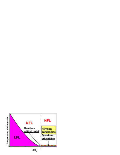
Figure 1: Schematic phase diagram of the system driven to the FC state. The number density $x$ is taken as the control parameter and depicted as $x/x_{c}$. The quantum critical point (QCP), $x/x_{c}=1$, of FCQPT is shown by the arrow. At $x/x_{c}<1$ and sufficiently low temperatures, the system is in the Landau Fermi liquid (LFL) state as shown by the shadow area. At $T=0$ and beyond QCP, $x/x_{c}>1$, the system is at the quantum critical line depicted by the dash line and shown by the vertical arrow. The critical line is characterized by the FC state with finite superconducting order parameter $\kappa$. At any finite temperature, the order parameter $\kappa$ is destroyed and the entropy becomes discontinuous at $T_{c}=0$, the system undergoes the first order phase transition and exhibits the NFL behavior at $T>0$.

Schematic phase diagram of the system which is driven to FC by variation of $x$ is reported in Fig. 1. Upon approaching the critical density $x_{c}$ the system remains in LFL region at sufficiently low temperatures khodb ; obz , that is shown by the shadow area. At QCP $x_{c}$ shown by the arrow in Fig. 1, the system demonstrates the NFL behavior down to the lowest temperatures. Beyond QCP at finite temperatures the behavior is remaining the NFL one and is determined by the temperature-independent entropy $S_{0}$ yakov . In that case at $T\to 0$, the system is approaching a quantum critical line (shown by the vertical arrow and the dashed line in Fig. 1) rather than a quantum critical point. Upon reaching the quantum critical line from the above at $T\to 0$ the system undergoes the first order quantum phase transition, which is FCQPT taking place at $T_{c}=0$.

At $T>0$ the NFL state above the critical line, see Fig. 1, is strongly degenerated, therefore it is captured by the other states such as superconducting (for example, by the superconducting state in $\rm CeCoIn_{5}$ bi ; shag1 ; shag2 ) or by AF state (e.g. AF one in $\rm YbRh_{2}Si_{2}$ geg1 ; geg ; plaq ) lifting the degeneracy. The application of magnetic field $B>B_{c0}$ restores the LFL behavior, where $B_{c0}$ is a critical magnetic field, such that at $B>B_{c0}$ the system is driven towards its Landau Fermi liquid (LFL) regime geg1 ; geg ; shag2 . In some cases, for example in HF metal $\rm CeRu_{2}Si_{2}$, $B_{c0}=0$, see e.g. takah , while in $\rm YbRh_{2}Si_{2}$, $B_{c0}\simeq 0.06$ T geg1 ; geg . In our simple model $B_{c0}$ is taken as a parameter.

III Scaling behavior of the effective mass

Schematic phase diagram of the HF metal $\rm YbRh_{2}Si_{2}$ is reported in Fig. 2. Magnetic field $B$ is taken as the control parameter. The FC state and the region lying at $x/x_{c}\geq 1$, see Fig. 1, can be captured by the superconducting, ferromagnetic, antiferromagnetic (AF) etc. states lifting the degeneracy obz ; khodb . Since we consider the HF metal $\rm YbRh_{2}Si_{2}$ the AF state takes place geg1 ; geg as shown in Fig. 2. As seen from Fig. 2, at elevated temperatures and fixed magnetic field the NFL regime occurs, while rising $B$ again drives the system from NFL region to LFL one. Below we consider the transition region when at rising $B$ the system moves from NFL regime to LFL one along the dash-dot horizontal arrow, and at elevated $T$ it moves from LFL regime to NFL one along the solid vertical arrow.

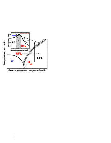
Figure 2: Schematic phase diagram of the HF metal $\rm YbRh_{2}Si_{2}$. $\rm{AF}$ denotes antiferromagnetic state. At $T=0$, $B_{c0}$ is magnetic field at which the effective mass diverges and the AF state vanishes. At $B>B_{c0}$ the system is in its paramagnetic state. The vertical arrow shows the transition from the LFL regime to the NFL one at fixed $B$ along $T$ with $M^{*}$ depending on $T$. The dash-dot horizontal arrow illustrates the system moving from NFL regime to LFL one along $B$ at fixed $T$. The inset shows a schematic plot of the scaling behavior of the normalized effective mass versus the normalized temperature. Transition regime, where $M^{*}_{N}$ reaches its maximum value $M^{*}_{M}$ at $T=T_{M}$, is shown by the hatched area both in the main panel and in the inset. The arrows mark the position of inflection point in $M^{*}_{N}$ and the transition region.

To explore a scaling behavior of $M^{*}$, we write the quasiparticle distribution function as $n_{1}({\bf p})=n({\bf p},T)-n({\bf p})$, with $n({\bf p})$ is the step function, and Eq. (3) then becomes

$$\frac{1}{M^{*}(T)}=\frac{1}{M^{*}}+\int\frac{{\bf p}_{F}{\bf p_{1}}}{p_{F}^{3}}F({\bf p_{F}},{\bf p}_{1})\frac{\partial n_{1}(p_{1},T)}{\partial p_{1}}\frac{d{\bf p}_{1}}{(2\pi)^{3}}.$$ (5)

At QCP the effective mass $M^{*}$ diverges and Eq. (5) becomes homogeneous determining $M^{*}$ as a function of temperature

$$M^{*}(T)\propto T^{-2/3},$$ (6)

while the system exhibits the NFL behavior ckz ; obz . If the system is located before QCP, $M^{*}$ is finite, at low temperatures the system demonstrates the LFL behavior that is $M^{*}(T)\simeq M^{*}+a_{1}T^{2}$, with $a_{1}$ is a constant, see the inset to Fig. 2. Obviously, the LFL behavior takes place when the second term on the right hand side of Eq. (5) is small in comparison with the first one. Then, at rising temperatures the system enters the transition regime: $M^{*}$ grows, reaching its maximum $M^{*}_{M}$ at $T=T_{M}$, with subsequent diminishing. Near temperatures $T\geq T_{M}$ the last ”traces” of LFL regime disappear, the second term starts to dominate, and again Eq. (5) becomes homogeneous, and the NFL behavior restores, manifesting itself in decreasing $M^{*}$ as $T^{-2/3}$, see Eq. (6). When the system is near QCP, it turns out that the solution of Eq. (5) $M^{*}(T)$ can be well approximated by a simple universal interpolating function obz ; ckz ; shag2 . The interpolation occurs between the LFL ($M^{*}\simeq M^{*}+a_{1}T^{2}$) and NFL ($M^{*}\propto T^{-2/3}$) regimes thus describing the above crossover ckz ; obz . Introducing the dimensionless variable $y=T_{N}=T/T_{M}$, we obtain the desired expression

$$M^{*}_{N}(y)\approx c_{0}\frac{1+c_{1}y^{2}}{1+c_{2}y^{8/3}}.$$ (7)

Here $M^{*}_{N}=M^{*}/M^{*}_{M}$ is the normalized effective mass, $c_{0}=(1+c_{2})/(1+c_{1})$, $c_{1}$ and $c_{2}$ are fitting parameters, parameterizing the Landau amplitude.

The inset to Fig. 2 demonstrates the scaling behavior of the normalized effective mass $M^{*}_{N}=M^{*}/M^{*}_{M}$ versus normalized temperature $T_{N}=T/T_{M}$, where $M^{*}_{M}$ is the maximum value that $M^{*}$ reaches at $T=T_{M}$. At $T\ll T_{M}$ the LFL regime takes place. At $T\gg T_{M}$ the $T^{-2/3}$ regime takes place. This is marked as NFL one since the effective mass depends strongly on temperature. The temperature region $T\simeq T_{M}$ signifies the transition between the LFL regime with almost constant effective mass and NFL behavior, given by $T^{-2/3}$ dependence. Thus temperatures $T\sim T_{M}$ can be regarded as the transition region between LFL and NFL regimes. The transition temperatures are not really a phase transition. These necessarily are broad, very much depending on the criteria for determination of the point of such a transition, as it is seen from the inset to Fig. 2. As usually, the transition temperature is extracted from the temperature dependence of charge transport, for example, from the resistivity $\rho(T)=\rho_{0}+AT^{2}$ with $\rho_{0}$ is the residual resistivity and $A$ is the LFL coefficient. The crossover takes place at temperatures where the resistance starts to deviate from the LFL $T^{2}$ behavior. Obviously, the measure of the deviation from the LFL $T^{2}$ behavior cannot be defined unambiguously. Therefore, different measures produce different results.

It is possible to transport Eq. (5) to the case of the application of magnetic fields ckz ; obz ; shag2 . The application of magnetic field restores the LFL behavior so that $M^{*}_{M}$ depends on $B$ as

$$M^{*}_{M}\propto(B-B_{c0})^{-2/3},$$ (8)

while

$$T_{M}\propto\mu_{B}(B-B_{c0}),$$ (9)

where $\mu_{B}$ is the Bohr magneton ckz ; shag2 ; obz . Employing Eqs. (8) and (9) to calculate $M^{*}_{M}$ and $T_{M}$, we conclude that Eq. (7) is valid to describe the normalized effective mass in external fixed magnetic fields with $y=T/(B-B_{c0})$. On the other hand, Eq. (7) is valid when the applied magnetic field becomes a variable, while temperature is fixed $T=T_{f}$. In that case, as seen from Eqs. (6), (7) and(8), it is convenient to rewrite both the variable as $y=(B-B_{c0})/T_{f}$, and Eq. (9) as

$$\mu_{B}(B_{M}-B_{c0})\propto T_{f}.$$ (10)

It follows from Eq. (7) that in contrast to the Landau paradigm of quasiparticles the effective mass strongly depends on $T$ and $B$. As we will see it is this dependence that forms the NFL behavior. It follows also from Eq. (7) that a scaling behavior of $M^{*}$ near QCP is determined by the absence of appropriate external physical scales to measure the effective mass and temperature. At fixed magnetic fields, the characteristic scales of temperature and of the function $M^{*}(T,B)$ are defined by both $T_{M}$ and $M^{*}_{M}$ respectively. At fixed temperatures, the characteristic scales are $(B_{M}-B_{c0})$ and $M^{*}_{M}$. It follows from Eqs. (8) and (9) that at fixed magnetic fields, $T_{M}\to 0$, and $M^{*}_{M}\to\infty$, and the width of the transition region shrinks to zero as $B\to B_{c0}$ when these are measured in the external scales. In the same way, it follows from Eqs. (6) and (10) that at fixed temperatures, $(B_{M}-B_{c0})\to 0$, and $M^{*}_{M}\to\infty$, and the width of the transition region shrinks to zero as $T_{f}\to 0$. Thus, the application of the external scales obscure the scaling behavior of the effective mass and of the thermodynamic and transport properties.

A few remarks are in order here. As we shall see, magnetic field dependencies of the effective mass or of other observable like the longitudinal magnetoresistance do not have ”peculiar points” like maximum. The normalization are to be performed in the other points like the inflection point at $T=T_{inf}$ (or at $B=B_{inf}$) shown in the inset to Fig. 2 by the arrow. Such a normalization is possible since it is established on the internal scales, $T_{inf}\propto T_{M}\propto(B-B_{c0})$.

IV NFL behavior of the HF metal $\rm\bf YbRh_{2}Si_{2}$

In what follows, we compute the effective mass and employ Eq. (7) for estimations of considered values. To compute the effective mass $M^{*}(T,B)$, we solve Eq. (5) with special form of Landau interaction amplitude, see Refs. ckz ; obz for details. Choice of the amplitude is dictated by the fact that the system has to be at QCP, which means that first two $p$-derivatives of the single-particle spectrum $\varepsilon({\bf p})$ should equal zero. Since first derivative is proportional to the reciprocal quasiparticle effective mass $1/M^{*}$, its zero just signifies QCP of FCQPT. Zero of the second derivative means that the spectrum $\varepsilon({\bf p})$ has an inflection point at $p_{F}$ rather than a maximum. Thus, the lowest term of the Taylor expansion of $\varepsilon({\bf p})$ is proportional to $(p-p_{F})^{3}$ ckz . After solution of Eq. (5), the obtained spectrum had been used to calculate the entropy $S(B,T)$, which, in turn, had been recalculated to the effective mass $M^{*}(T,B)$ by virtue of well-known LFL relation $M^{*}(T,B)=S(T,B)/T$. Our calculations of the normalized entropy as a function of the normalized magnetic field $B/B_{inf}=y$ and as a function of the normalized temperature $y=T/T_{inf}$ are reported in Fig. 3. Here $T_{inf}$ and $B_{inf}$ are the corresponding inflection points in function $S$. We normalize the entropy by its value at the inflection point $S_{N}(y)=S(y)/S(1)$. As seen form Fig. 3, our calculations corroborate the scaling behavior of the normalized entropy, that is the curves at different temperatures and magnetic fields merge into single one in terms of the variable $y$. The inflection point $T_{inf}$ in $S(T)$ makes $M^{*}(T,B)$ have its maximum as a function of $T$, while $M^{*}(T,B)$ versus $B$ has no maximum. We note that our calculations of the entropy confirm the validity of Eq. (7) and the scaling behavior of the normalized effective mass.

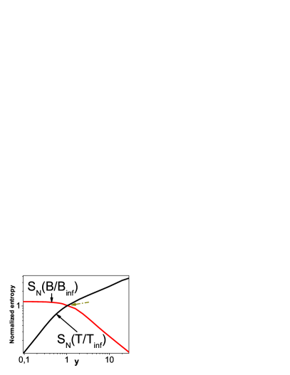
Figure 3: The normalized entropy $S_{N}(B/B_{inf})$ versus $y=B/B_{inf}$ and the normalized entropy $S_{N}(T/T_{inf})$ versus $y=T/T_{inf}$ calculated at fixed temperature and magnetic field, correspondingly, are represented by the solid lines and shown by the arrows. The inflection point is depicted by the dash-dot arrow.

IV.1 Heat capacity

Exciting measurements of $C/T\propto M^{*}$ on samples of the new generation of $\rm YbRh_{2}Si_{2}$ in different magnetic fields $B$ up to 1.5 T oes allow us to identify the scaling behavior of the effective mass $M^{*}$ and observe the different regimes of $M^{*}$ behavior such as the LFL regime, transition region from LFL to NFL regimes, and the NFL regime itself. A maximum structure in $C/T\propto M^{*}_{M}$ at $T_{M}$ appears under the application of magnetic field $B$ and $T_{M}$ shifts to higher $T$ as $B$ is increased. The value of $C/T=\gamma_{0}$ is saturated towards lower temperatures decreasing at elevated magnetic field, where $\gamma_{0}$ is the Sommerfeld coefficient oes .

The transition region corresponds to the temperatures where the vertical arrow in the main panel of Fig. 2 crosses the hatched area. The width of the region, being proportional to $T_{M}\propto(B-B_{c0})$ shrinks, $T_{M}$ moves to zero temperature and $\gamma_{0}\propto M^{*}$ increases as $B\to B_{c0}$. These observations are in accord with the facts oes .

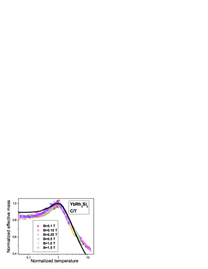
Figure 4: The normalized effective mass $M^{*}_{N}$ extracted from the measurements of the specific heat $C/T$ on $\rm YbRh_{2}Si_{2}$ in magnetic fields $B$ oes listed in the legend. Our calculations are depicted by the solid curve tracing the scaling behavior of $M^{*}_{N}$.

To obtain the normalized effective mass $M^{*}_{N}$, the maximum structure in $C/T$ was used to normalize $C/T$, and $T$ was normalized by $T_{M}$. In Fig. 4 $M^{*}_{N}$ as a function of normalized temperature $T_{N}$ is shown by geometrical figures, our calculations are shown by the solid line. Figure 4 reveals the scaling behavior of the normalized experimental curves - the scaled curves at different magnetic fields $B$ merge into a single one in terms of the normalized variable $y=T/T_{M}$. As seen, the normalized mass $M^{*}_{N}$ extracted from the measurements is not a constant, as would be for LFL. The two regimes (the LFL regime and NFL one) separated by the transition region, as depicted by the hatched area in the inset to Fig. 2, are clearly seen in Fig. 4 illuminating good agreement between the theory and the facts. It is worthy of note that the normalization procedure allows us to construct the scaled function $C/T$ extracted from the facts in wide range variation of the normalized temperature. Indeed, it integrates measurements of $C/T$ taken at the application of different magnetic fields into unique function which demonstrates the scaling behavior over three decades in normalized temperature as seen from Fig. 4.

IV.2 Magnetization

Consider now the magnetization $M$ as a function of magnetic field $B$ at fixed temperature $T=T_{f}$

$$M(B,T)=\int_{0}^{B}\chi(b,T)db,$$ (11)

where the magnetic susceptibility $\chi$ is given by land

$$\chi(B,T)=\frac{\beta M^{*}(B,T)}{1+F_{0}^{a}}.$$ (12)

Here, $\beta$ is a constant and $F_{0}^{a}$ is the Landau amplitude related to the exchange interaction land . In the case of strongly correlated systems $F_{0}^{a}\geq-0.9$ pfit ; pfit1 . Therefore, as seen from Eq. (12), due to the normalization the coefficients $\beta$ and $(1+F_{0}^{a})$ drops out from the result, and $\chi\propto M^{*}$.

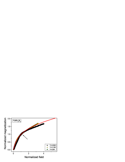
Figure 5: The field dependencies of the normalized magnetization $M$ collected at different temperatures shown at right bottom corner are extracted from measurements collected on $\rm{YbRu_{2}Si_{2}}$ steg . The kink (shown by the arrow) is clearly seen at the normalized field $B_{N}=B/B_{k}\simeq 1$. The solid curve represents our calculations.

One might suppose that $F_{0}^{a}$ can strongly depend on $B$. This is not the case, since the Kadowaki-Woods ratio is conserved kadw ; geg1 ; kwz ; natphys , $A(B)/\gamma_{0}^{2}(B)\propto A(B)/\chi^{2}(B)\propto const$, we have $\gamma_{0}\propto M^{*}\propto\chi$. Here $A$ is the coefficient in the $T^{2}$ dependence of resistivity $\rho$.

Our calculations show that the magnetization exhibits a kink at some magnetic field $B=B_{k}$. The experimental magnetization demonstrates the same behavior steg . We use $B_{k}$ and $M(B_{k})$ to normalize $B$ and $M$ respectively. The normalized magnetization $M(B)/M(B_{k})$ extracted from facts steg depicted by the geometrical figures and calculated magnetization shown by the solid line are reported in Fig. 5. As seen, the scaled data at different $T_{f}$ merge into a single one in terms of the normalized variable $y=B/T_{k}$. It is also seen, that these exhibit energy scales separated by kink at the normalized magnetic field $B_{N}=B/B_{k}=1$. The kink is a crossover point from the fast to slow growth of $M$ at rising magnetic field. It is seen from Fig. 5, that our calculations are in good agreement with the facts, and all the data exhibit the kink (shown by the arrow) at $B_{N}\simeq 1$ taking place as soon as the system enters the transition region corresponding to the magnetic fields where the horizontal dash-dot arrow in the main panel of Fig. 2 crosses the hatched area. Indeed, as seen from Fig. 5, at lower magnetic fields $M$ is a linear function of $B$ since $M^{*}$ is approximately independent of $B$. Then, it follows from Eqs. (7) and (8) that at elevated magnetic fields $M^{*}$ becomes a diminishing function of $B$ and generates the kink in $M(B)$ separating the energy scales discovered in Refs. steg1 ; steg . Then, as seen from Eq. (10) the magnetic field $B_{k}$ at which the kink appears, $B_{k}\simeq B_{M}\propto T_{f}$, shifts to lower $B$ as $T_{f}$ is decreased. This observation is in accord with the facts steg1 ; steg .

IV.3 Longitudinal magnetoresistance

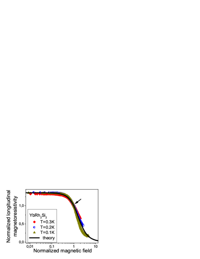
Figure 6: Magnetic field dependence of the normalized magnetoresistance $\rho_{N}$ versus normalized magnetic field. $\rho_{N}$ was extracted from LMR of $\rm YbRh_{2}Si_{2}$ at different temperatures steg1 ; steg listed in the legend. The inflection point is shown by the arrow, and the solid line represents our calculations.

Consider a longitudinal magnetoresistance (LMR) $\rho(T,B)=\rho_{0}+A(T,B)T^{2}$ as a function of $B$ at fixed $T=T_{f}$. In that case, the classical contribution to LMR due to orbital motion of carriers induced by the Lorentz force is small, while the Kadowaki-Woods relation kadw ; geg1 ; kwz ; natphys , $K=A/\gamma_{0}^{2}\propto A/\chi^{2}=const$, allows us to employ $M^{*}$ to construct the coefficient $A$ pla3 , since $\gamma_{0}\propto\chi\propto M^{*}$. As a result, $\rho(T,B)-\rho_{0}\propto(M^{*})^{2}$. Fig. 6 reports the normalized magnetoresistance

$$\rho_{N}(y)=\frac{\rho(y)-\rho_{0}}{\rho_{inf}}\propto(M_{N}^{*}(y))^{2}$$ (13)

versus normalized magnetic field $y=B/B_{inf}$ at different temperatures, shown in the legend. Here $\rho_{inf}$ and $B_{inf}$ are LMR and magnetic field respectively taken at the inflection point marked by the arrow in Fig. 6. Both theoretical (shown by the solid line) and experimental (marked by the geometrical figures) curves have been normalized by their inflection points, which also reveals the scaling behavior - the scaled curves at different temperatures merge into single one as a function of the variable $y$ and show the scaling behavior over three decades in the normalized magnetic field. The transition region at which LMR starts to decrease is shown in the inset to Fig. 2 by the hatched area. Obviously, as seen from Eq. (10), the width of the transition region being proportional to $B_{M}\simeq B_{inf}\propto T_{f}$ decreases as the temperature $T_{f}$ is lowered. In the same way, the inflection point of LMR, generated by the inflection point of $M^{*}$ shown in the inset to Fig. 2 by the arrow, shifts to lower $B$ as $T_{f}$ is decreased. All these observations are in excellent agreement with the facts steg1 ; steg .

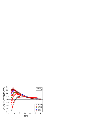
Figure 7: MR versus temperature $T$ as a function of magnetic field $B$. The experimental data on MR were collected on $\rm{CeCoIn_{5}}$ at fixed magnetic field $B$ pag shown in the right bottom corner of the Figure. The solid lines represent our calculations.

It is instructive to demonstrate that the same effective mass employed to calculate LMR shown in Fig. 6 gives good description of the magnetoresistance (MR) collected in measurements on $\rm{CeCoIn_{5}}$. Figure 7 shows the calculated MR versus temperature as a function of magnetic field $B$ together with the experimental points from Ref. pag . We note that both the classical contribution to MR due to orbital motion of carriers induced by the Lorentz force and $\rho_{0}$ were omitted. As seen from Fig. 7, our description of experiment is pretty good plamr .

IV.4 Magnetic entropy

The evolution of the derivative of magnetic entropy $dS(B,T)/dB$ as a function of magnetic field $B$ at fixed temperature $T_{f}$ is of great importance since it allows us to study the scaling behavior of the derivative of the effective mass $TdM^{*}(B,T)/dB\propto dS(B,T)/dB$. While the scaling properties of the effective mass $M^{*}(B,T)$ can be analyzed via LMR, see Fig. 6.

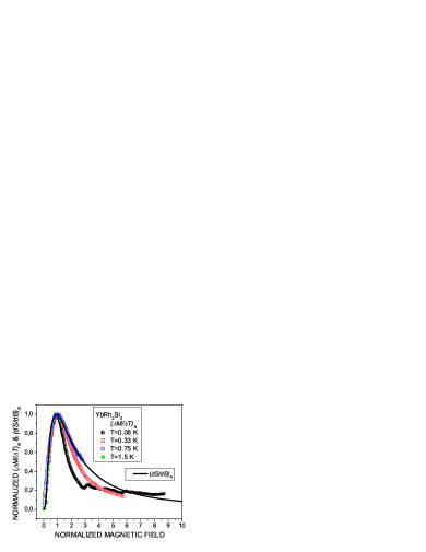
Figure 8: Normalized magnetization difference divided by temperature increment $(\Delta M/\Delta T)_{N}$ versus normalized magnetic field at fixed temperatures listed in the legend is extracted from the facts collected on $\rm YbRh_{2}Si_{2}$ geg . Our calculation of the normalized derivative $(dS/dB)_{N}\simeq(\Delta M/\Delta T)_{N}$ versus normalized magnetic field is shown by the solid line.

As seen from from Eqs. (7) and (10), at $y\leq 1$ the derivative $-dM_{N}(y)/dy\propto y$ with $y=(B-B_{c0})/(B_{inf}-B_{c0})\propto(B-B_{c0})/T_{f}$. We note that the effective mass as a function of $B$ does not have the maximum. At elevated $y$ the derivative $-dM_{N}(y)/dy$ possesses a maximum at the inflection point and then becomes a diminishing function of $y$. Upon using the variable $y=(B-B_{c0})/T_{f}$, we conclude that at decreasing temperatures, the leading edge of the function $-dS/dB\propto-TdM^{*}/dB$ becomes steeper and its maximum at $(B_{inf}-B_{c0})\propto T_{f}$ is higher. These observations are in quantitative agreement with striking measurements of the magnetization difference divided by temperature increment, $-\Delta M/\Delta T$, as a function of magnetic field at fixed temperatures $T_{f}$ collected on $\rm YbRh_{2}Si_{2}$ geg . We note that according to the well-know thermodynamic equality $dM/dT=dS/dB$, and $\Delta M/\Delta T\simeq dS/dB$. To carry out a quantitative analysis of the scaling behavior of $-dM^{*}(B,T)/dB$, we calculate the normalized entropy $S$ shown in Fig. 3 as a function of $B/B_{inf}$ at fixed temperature $T_{f}$. Fig. 8 reports the normalized $(dS/dB)_{N}$ as a function of the normalized magnetic field. The scaled function $(dS/dB)_{N}$ is obtained by normalizing $(-dS/dB)$ by its maximum taking place at $B_{M}$, and the field $B$ is scaled by $B_{M}$. The measurements of $-\Delta M/\Delta T$ are normalized in the same way and depicted in Fig. 8 as $(\Delta M/\Delta T)_{N}$ versus normalized field. It is seen from Fig. 8 that our calculations shown by the solid line are in good agreement with the facts and the scaled functions $(\Delta M/\Delta T)_{N}$ extracted from the facts show the scaling behavior in wide range variation of the normalized magnetic field $B/B_{M}$.

IV.5 Energy scales and $T-B$ phase diagram for $\rm\bf YbRh_{2}Si_{2}$

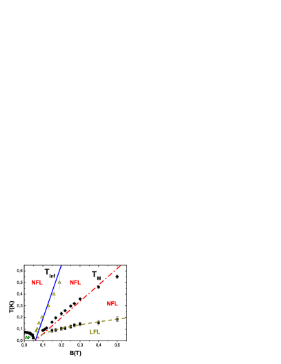
Figure 9: Temperature versus magnetic field $T-B$ phase diagram for $\rm YbRh_{2}Si_{2}$. Solid circles represent the boundary between AF and NFL states. The solid squares denote the boundary of the NFL and LFL regime steg1 ; steg ; geg1 shown by the dotted line which is approximated by $\sqrt{B-B_{c0}}$ obz . Diamonds mark the maximums $T_{M}$ of $C/T$ oes shown in Fig. 4. The dash-dot line is approximated by $T_{M}\propto a(B-B_{c0})$, $a$ is a fitting parameter, see Eq. (9). Triangles along the solid line denote $T_{inf}$ in LMR steg1 ; steg sown in Fig. 8, the solid line represents the function $T_{inf}\propto b(B-B_{c0})$, $b$ is a fitting parameter, see Eq. (10).

Fig. 9 reports $T_{inf}$ and $T_{M}$ versus $B$ depicted by the solid and dash-dotted lines, respectively. The boundary between the NFL and LFL regimes is shown by the dashed line, and AF marks the antiferromagnetic state. The corresponding data are taken from Ref. steg1 ; steg ; oes ; geg1 . It is seen that our calculations are in good agreement with the facts jetpl . In Fig. 9, the solid and dash-dotted lines corresponding to the functions $T_{inf}$ and $T_{M}$, respectively, represent the positions of the kinks separating the energy scales in $C$ and $M$ reported in Ref. steg1 ; steg . It is seen that our calculations are in accord with facts, and we conclude that the energy scales are reproduced by Eqs. (9) and (10) and related to the peculiar points of the normalized effective mass $M^{*}_{N}$. The points are the inflection point $T_{inf}$ and the maximum point $T_{M}$ at which the transition region is located. These are shown by the arrows in the inset to Fig. 2.

At $B\to B_{c0}$ both $T_{inf}\to 0$ and $T_{M}\to 0$, thus the LFL and the transition regimes of both $C/T$ and $M$ as well as these of LMR and the magnetic entropy are shifted to very low temperatures. Therefore due to experimental difficulties these regimes cannot be often observed in experiments on HF metals. As it is seen from Figs. 4, 5, 6, 8 and 9, the normalization allows us to construct the unique scaled thermodynamic and transport functions extracted from the experimental facts in wide range of the variation of the scaled variable $y$. As seen from the mentioned Figures, the constructed normalized thermodynamic and transport functions show the scaling behavior over three decades in the normalized variable.

V Universal Behavior of Two-Dimensional $\rm\bf{}^{3}He$ at Low Temperatures

The bulk liquid $\rm{}^{3}He$ is historically the first object, to which the Landau Fermi-liquid (LFL) theory had been applied land . This substance, being an intrinsically isotropic Fermi-liquid with negligible spin-orbit interaction is ideal to test the LFL theory. It is remarkable that the same ³He becomes the first 2D homogeneous Fermi-liquid in which the NFL behavior has been detected he3 ; he3a ; prlhe . 2D ³He has a very important feature: a change of the number density $x$ of ³He film drives it towards QCP at which the quasiparticle effective mass $M^{*}$ diverges he3 ; he3a ; prlhe . This peculiarity permits to plot the experimental temperature-density phase diagram, which can be directly compared with the theoretical phase diagram shown in Fig. 1. As a result, 2D $\rm{}^{3}He$ becomes an ideal system to test a theory describing the NFL behavior. Namely, the neutral atoms of $\rm{}^{3}He$ are fermions interacting with each other by Van-der-Vaals forces with strong hardcore repulsion and a weakly attractive tail. The different character of inter-particle interaction along with the fact, that the mass of $\rm{}^{3}He$ atom is 3 orders of magnitude larger than that of an electron, makes $\rm{}^{3}He$ systems to have drastically different properties than those of HF metals. Because of this difference nobody can be sure that the macroscopic physical properties of these systems will be more or less similar to each other at their QCP.

In this Section we show that despite of very different microscopic nature of 2D ³He and 3D HF metals, their main universal features at their QCP are the same, being dictated by the extended quasiparticles paradigm. Our analysis of the experimental measurements has shown that the behavior of 2D ³He is quite similar to that of HF compounds with various ground state magnetic properties. Namely, we demonstrate that the main universal features of $\rm{}^{3}He$ experimental $T$-$x$ phase diagram resemble those in HF metals and can be well captured utilizing the notion of FCQPT embracing the extended quasiparticles paradigm and thus deriving NFL properties of above systems from the paradigm. We also show that the universal behavior of the effective mass of 2D $\rm{}^{3}He$ coincides with that observed in HF metals.

V.1 The temperature-number density phase diagram of 2D $\rm{}^{3}He$

As we seen in Section I, at QCP $x=x_{c}$ the effective mass diverges at $T=0$ and the leading term of this divergence given by Eq. (4) reads

$$\frac{M^{*}(x)}{M}=A+\frac{B}{1-z},\ z=\frac{x}{x_{c}}.$$ (14)

Equation (14) is valid in both 3D and 2D cases, while the values of factors $A$ and $B$ depend on dimensionality and inter-particle interaction obz . At $x>x_{c}$ the fermion condensation takes place. Here we confine ourselves to the case $x<x_{c}$.

Equation (14) shows that the maximum value of the effective mass $M^{*}_{M}\propto 1/(1-z)$ and it follows from (6) that $M^{*}_{M}\propto T^{-2/3}$. As a result, we obtain that $T_{M}$ at which the effective mass reaches its maximum value $M^{*}_{M}\propto T^{-2/3}$ is given by

$$T_{M}\propto(1-z)^{3/2}.$$ (15)

We note that obtained results are in agreement with numerical calculations obz ; ckz .

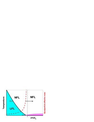
Figure 10: The temperature-number density phase diagram of 2D $\rm{}^{3}He$. The part for $z<1$ corresponds to HF behavior divided into the LFL and NFL parts by the line $T_{M}(z)\propto(1-z)^{3/2}$, where $T_{M}$ is the effective mass maximum temperature. The exponent $3/2=1.5$ coming from Eq. (15) is in good agreement with the experimental value of $1.7\pm 0.1$ he3 . The dependence $M^{*}(z)\propto(1-z)^{-1}$ shown by the dashed line points out QCP taking place at $z=1$. The regime for $z\geq 1$ consists of the LFL piece (the shadowed region, beginning in the intervening phase $z\leq 1$ he3 , which is due to the substrate inhomogeneities, see text) and the NFL regime at higher temperatures.

In Fig. 10, we show the phase diagram of 2D ³He in the variables $T$ - $z$ (see Eq. (14)). For the sake of comparison the plot of the effective mass versus $z$ is shown by dashed line. The dependence $M^{*}(z)\propto(1-z)^{-1}$ demonstrates that the effective mass diverges at QCP with $z=1$ in accordance with the general phase diagram displayed in Fig. 1. The part of the diagram where $z<1$ corresponds to HF behavior and consists of LFL and NFL parts, divided by the line $T_{M}(z)\propto(1-z)^{3/2}$. We draw attention here, that our exponents $1$ (see Eq. (14)) and $3/2=1.5$ (see Eq. (15)) are in good agreement with these from Ref. he3 . The good coincidence between the theoretical and experimental exponents speaks in favor of realization of our FCQPT scenario in the NFL behavior of both 2D ³He and HF metals as former system is in great detail similar to them.

The regime for $z>1$ located above the quantum critical line, see Figs. 10 and 1, consists of low-temperature LFL piece, (shown in Fig. 10 by shadowed region, beginning in the intervening phase $z\leq 1$ he3 ) and NFL regime at higher temperatures. The former LFL piece is related to the peculiarities of substrate on which 2D $\rm{}^{3}He$ film is placed. Namely, it is related to weak substrate heterogeneity (steps and edges on its surface) so that quasiparticles, being localized (pinned) on it, give rise to the LFL behavior he3 ; he3a . That is the peculiarities of the substrate eliminate the degeneracy generated by the FC state taking place at $z>1$ in the same way as the AF state does in the case of $\rm YbRh_{2}Si_{2}$, see Fig. 2. At elevated temperatures, the competition between thermal and pinning energies returns the system back to the unpinned state restoring the NFL behavior. As HF metals do not have a substrate, the LFL behavior is induced by the AF state lifting the degeneracy. At elevated temperatures, this state is destroyed and exhibits the NFL behavior, as it is shown in Fig. 2. If the AF state were absent and some disorder (like point defects, dislocations etc) were present in the lattice a rather thin LFL piece could take place at low temperatures.

V.2 NFL behavior of 2D $\rm\bf{}^{3}He$ versus that of HF metals

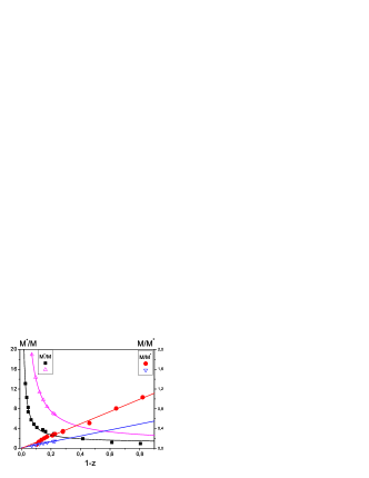
Figure 11: The dependence of the effective mass $M^{*}(z)$ on the dimensionless density $1-z=1-x/x_{c}$. Experimental data from Ref. prlhe are shown by circles and squares and those from Ref. he3 are shown by triangles. The effective mass is fitted as $M^{*}(z)/M\propto A+B/(1-z)$ (see Eq. (14)), while the reciprocal one as $M/M^{*}(z)\propto A_{1}z$, where $A,B$ and $A_{1}$ are constants.

As we have seen above, $M^{*}(T)$ can be measured in experiments on strongly correlated Fermi-systems. For example, $M^{*}(T)\propto C(T)/T\propto S(T)/T\propto M_{0}(T)\propto\chi(T)$ where $C(T)$ is the specific heat, $S(T)$ — entropy, $M_{0}(T)$ — magnetization and $\chi(T)$ — AC magnetic susceptibility. If the measurements are performed at fixed $x$ then, as it follows from Eq. (7), the effective mass reaches the maximum at $T=T_{M}$. Upon normalizing both $M^{*}(T)$ by its peak value at each $x$ and the temperature by $T_{M}$, we see from Eq. (7) that in the case of 2D $\rm{}^{3}He$ all the curves also merge a into single one, demonstrating a scaling behavior.

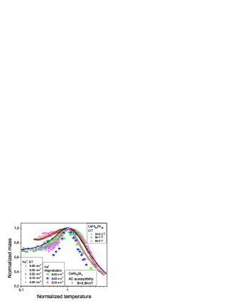
Figure 12: The normalized effective mass $M^{*}_{N}$ as a function of the normalized temperature $T/T_{M}$ at densities shown in the left bottom corner. The behavior of $M^{*}_{N}$ is extracted from experimental data obtained in 2D ³He he3a and 3D HF compounds with different magnetic ground states such as $\rm{CeRu_{2}Si_{2}}$ and $\rm CePd_{1-x}Rh_{x}$ pikul ; takah , fitted by the solid curve given by (7).

In Fig. 11, we report the experimental values of effective mass $M^{*}(z)$ obtained by the measurements on ³He monolayer prlhe . These measurements, in coincidence with those from Ref. he3 , show the divergence of the effective mass at $x=x_{c}$. To show that our FCQPT approach is able to describe the above data, we represent the fit of $M^{*}(z)$ by the fractional expression $M^{*}(z)/M\propto A+B/(1-z)$ and the reciprocal effective mass by the linear fit $M/M^{*}(z)\propto A_{1}z$. We note here, that the linear fit has been used to describe the experimental data for a bilayer of ³He he3 and we use this function here for the sake of illustration. It is seen from Fig. 11 that the data he3 (³He bilayer) can be equally well approximated by both linear and fractional functions, while the data prlhe cannot. For instance, both fitting functions give for the critical density in bilayer $x_{c}\approx 9.8$ nm^-2, while for monolayer prlhe these values are different: $x_{c}=5.56$ for a linear fit and $x_{c}=5.15$ for a fractional fit. It is seen from Fig. 11, that a linear fit is unable to properly describe the experiment prlhe at small $1-z$ (i.e. near $x=x_{c}$), while the fractional fit describes the experiment very well. This means that more detailed measurements are necessary in the vicinity $x=x_{c}$.

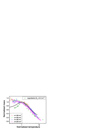
Figure 13: The dependence $M^{*}_{N}(T/T_{M})$ at densities shown in the left down corner. The behavior $M^{*}_{N}$ is extracted from experimental data for $C(T)/T$ in 2D ³He prlhe and for the magnetization $M_{0}$ in 2D ³He he3 . The solid curve shows the universal function, see the caption to Fig. 12.

We now apply the universal dependence (7) to fit the experiment not only in 2D ³He but also in 3D HF metals. $M^{*}_{N}(y)$ extracted from the entropy $S(T)/T$ and magnetization $M_{0}$ measurements on the ³He film he3a at different densities $x<x_{c}$ is reported in Fig. 12. In the same figure, the data extracted from the heat capacity of ferromagnet CePd_0.2Rh_0.8 pikul and the AC magnetic susceptibility of paramagnet CeRu₂Si₂ takah are plotted for different magnetic fields. It is seen that the universal behavior of the normalized effective mass given by Eq. (7) and shown by the solid curve is in accord with the experimental facts. All 2D ³He substances are located at $x<x_{c}$, where the system progressively disrupts its LFL behavior at elevated temperatures. In that case the control parameter, driving the system towards its QCP $x_{c}$ is merely the number density $x$. It is seen that the behavior of $M^{*}_{N}(y)$, extracted from $S(T)/T$ and $M_{0}$ of 2D ³He (the entropy $S(T)$ is reported in Fig. S8 A of Ref. he3a ) looks very much like that of 3D HF compounds. As we shall see from Fig. 14 below, the amplitude and positions of the maxima of magnetization $M_{0}(T)$ and $S(T)/T$ in 2D ³He follow nicely Eqs. (14) and (15). We conclude that Eq. (7) allows for the reduction of a 4D function describing the effective mass to a function of a single variable. Indeed, the effective mass depends on the magnetic field, temperature, number density and composition so that all these parameters can be merged in the single variable by means of interpolating function like Eq. (7).

The attempt to fit the available experimental data for $C(T)/T$ in 2D $\rm{}^{3}He$ prlhe by the universal function $M^{*}_{N}(y)$ is reported in Fig. 13. Here, the data extracted from heat capacity $C(T)/T$ for the ³He monolayer prlhe and magnetization $M_{0}$ for the bilayer he3 , are reported. It is seen that the effective mass extracted from these thermodynamic quantities can be well described by the universal interpolation formula (7). We note the qualitative and quantitative similarity between the double layer he3 and the monolayer prlhe of ³He as seen from Fig. 13.

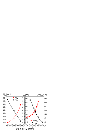
Figure 14: Left panel, the peak temperatures $T_{M}$ and the peak values $M_{\rm max}$ extracted from measurements of the magnetization $M_{0}$ in ³He he3 . Right panel shows $T_{M}$ and the peak values $(S/T)_{\rm max}$ extracted from measurements of $S(T)/T$ in ³He he3a . We approximate $T_{M}\propto(1-z)^{3/2}$ and $(S/T)_{\rm max}\propto M_{\rm max}\propto A/(1-z)$.

In the left panel of Fig. 14, we show the density dependence of $T_{M}$, extracted from measurements of the magnetization $M_{0}(T)$ of the ³He bilayer he3 . The peak temperature is fitted by Eq. (15). In the same Figure, we have also reported the maximal magnetization $M_{\rm max}$. It is seen that $M_{\rm max}$ is well described by the expression $M_{\rm max}\propto(S/T)_{\rm max}\propto(1-z)^{-1}$, see Eq. (14). The right panel of Fig. 14 reports the peak temperature $T_{M}$ and the maximal entropy $(S/T)_{\rm max}$ versus the number density $x$. They are extracted from the measurements of $S(T)/T$ on the ³He bilayer he3a . The fact that both the left and right panels exhibit the same behavior of the curves shows once more that there are indeed the quasiparticles, determining the thermodynamic behavior of 2D ³He near its QCP related to FCQPT.

VI Summary

We have analyzed the non-Fermi liquid behavior of the heavy fermion metals, and showed that extended quasiparticles paradigm is strongly valid, while the dependence of the effective mass on temperature, number density and applied magnetic fields gives rise to the NFL behavior. We have demonstrated that our theoretical study of the heat capacity, magnetization, longitudinal magnetoresistance and magnetic entropy are in good agreement with the outstanding recent facts collected on the HF metal $\rm YbRh_{2}Si_{2}$. Our normalization procedure has allowed us to construct the scaled thermodynamic and transport properties in wide range of the variation of the scaled variable. For $\rm YbRh_{2}Si_{2}$ the constructed thermodynamic and transport functions show the scaling behavior over three decades in the normalized variable. The energy scales in these functions are also explained.

We have described the diverse experimental facts related to temperature and number density dependencies of the thermodynamic characteristics of 2D ³He by a single universal function of one argument. The above universal behavior is also inherent to HF metals with different magnetic ground states. We obtain the marvelous coincidence with experiment in the framework of our theory. Moreover, these data could be obtained for 2D ³He only and thus they were inaccessible for analysis in HF metals. This fact also shows the universality of our approach. Thus we have shown that bringing the experimental data collected on different strongly correlated Fermi-systems to the above form immediately reveals their universal scaling behavior. Thus, the theory of fermion condensation quantum phase transition, preserving the extended quasiparticles paradigm and intimately related to unlimited growth of the effective mass as a function of temperature, magnetic field etc, is capable of describing the strongly correlated Fermi systems.

VII Acknowledgement

This work was supported in part by RFBR No. 09-02-00056.

References

- (1) G.R. Stewart, Rev. Mod. Phys. 73, 797 (2001).
- (2) H. v. Löhneysen, A. Rosch, M. Vojta, P. Wölfle, Rev. Mod. Phys. 79, 1015 (2007).
- (3) P. Gegenwart, Q. Si, and F. Steglich, Nature Phys. 4, 186 (2008).
- (4) S. Sachdev, Nature Phys. 4, 173 (2008).
- (5) P. Coleman and A.J. Schofield, Nature 433, 226 (2005).
- (6) P. Coleman et al., J. Phys. Condens. Matter 13, R723 (2001).
- (7) V.A. Khodel, JETP Lett. 86, 721 (2007); V.A. Khodel, J.W. Clark, and M.V. Zverev, arXiv: 0904.1509
- (8) V.A. Khodel and V.R. Shaginyan, JETP Lett. 51, 553 (1990).
- (9) M. Ya. Amusia and V.R. Shaginyan, Phys. Rev. B 63, 224507 (2001).
- (10) J. Dukelsky et. al., Z. Phys. B: Condens. Matter 102, 245 (1997).
- (11) G.E. Volovik, Quantum Phase Transitions from Topology in Momentum Space, Lect. Notes in Physics 718, 31 (2007).
- (12) V.R. Shaginyan, M.Ya. Amusia, and K.G. Popov, Physics-Uspekhi 50, 563 (2007).
- (13) V.A. Khodel, J.W. Clark, and M.V. Zverev, Phys. Rev. B 78, 075120 (2008).
- (14) V.R. Shaginyan et. al., Phys. Rev. Lett. 100, 096406 (2008).
- (15) J.W. Clark, V.A. Khodel, and M.V. Zverev Phys. Rev. B 71, 012401 (2005).
- (16) V.R. Shaginyan, M.Ya. Amusia, and K.G. Popov, Phys. Lett. A 373, 2281 (2009).
- (17) V.R. Shaginyan, M.Ya. Amusia, K.G. Popov, and S.A. Artamonov, JETP Lett. 90, 47 (2009).
- (18) P. Gegenwart et. al., Science 315, 969 (2007).
- (19) N. Oeschler et. al., Physica B 403, 1254 (2008).
- (20) P. Gegenwart et. al., Physica B 403, 1184 (2008).
- (21) Y. Tokiwa et. al., Phys. Rev. Lett. 102, 066401 (2009).
- (22) L.N. Oliveira, E.K.U. Gross, and W. Kohn, Phys. Rev. Lett. 60, 2430 (1988).
- (23) V.R. Shaginyan et. al., Europhys. Lett. 76, 898 (2006).
- (24) V.A. Khodel, M.V. Zverev, and V.M. Yakovenko, Phys. Rev. Lett. 95, 236402 (2005).
- (25) V.R. Shaginyan, Phys. Lett. A 249, 237 (1998).
- (26) E.M. Lifshitz and L.P. Pitaevskii, Statistical Physics, Part 2, Butterworth-Heinemann, Oxford, 1999.
- (27) M. Pfitzner and P. Wölfle, Phys. Rev. B 33, 2003 (1986).
- (28) D. Wollhardt, P. Wölfle, and P.W. Anderson, Phys. Rev. B 35, 6703 (1987).
- (29) A. Bianchi et al., Phys. Rev. Lett. 91, 257001 (2003); F. Ronning et al., Phys. Rev. B 71, 104528 (2005).
- (30) V.R. Shaginyan, K.G. Popov, and V.A. Stephanovich, Europhys. Lett. 79, 47001 (2007).
- (31) P. Gegenwart, et al., Phys. Rev. Lett. 89, 056402 (2002).
- (32) D. Takahashi et al., Phys. Rev. B 67, 180407(R) (2003).
- (33) K. Kadowaki and S.B. Woods, Solid State Commun. 58, 507 (1986).
- (34) A. Khodel and P. Schuck, Z. Phys. B: Condens. Matter 104, 505 (1997).
- (35) A.C. Jacko, J.O. Fjærestad, B.J. Powell, Nature Physics 5 (2009) 422.
- (36) V.R. Shaginyan et al., Phys. Lett. A 373, 986 (2009).
- (37) J. Paglione, et. al., Phys. Rev. Lett. 91 246405 (2003).
- (38) V.R. Shaginyan, M.Ya. Amusia, A.Z. Msezane, K.G. Popov, and V.A. Stephanovich, Phys. Lett. A 373, 986 (2009).
- (39) M. Neumann, J. Nyéki, and J. Saunders, Science 317, 1356 (2007).
- (40) Supporting online material for Ref. he3 .
- (41) A. Casey, H. Patel, J. Nyéki, B. P. Cowan, and J. Saunders, Phys. Rev. Lett. 90, 115301 (2003).
- (42) A.P. Pikul et al., J. Phys. Condens. Matter 18, L535 (2006).