Parameter-free density functional for the correlation energy in two dimensions

Abstract

Accurate treatment of the electronic correlation in inhomogeneous electronic systems, combined with the ability to capture the correlation energy of the homogeneous electron gas, allows to reach high predictive power in the application of density-functional theory. For two-dimensional systems we can achieve this goal by generalizing our previous approximation [Phys. Rev. B 79, 085316 (2009)] to a parameter-free form, which reproduces the correlation energy of the homogeneous gas while preserving the ability to deal with inhomogeneous systems. The resulting functional is shown to be very accurate for finite systems with an arbitrary number of electrons with respect to numerically exact reference data.

I Introduction

With the present technology, electron gas can be confined in various ways to create nanoscale devices of lower dimensionality. In particular, the field of two-dimensional (2D) physics has grown rapidly alongside the development of electronic (quasi-)2D devices such as quantum Hall bars and point contacts, and semiconductor quantum dots (QDs). In the modeling of QDs, the most common and usually valid approach is to consider a purely 2D Hamiltonian with a standard, (not screened nor softened) Coulomb interaction and effective values for the electron mass and dielectric constant, which account for the surrounding semiconducting material such as GaAs. qd

QDs are studied theoretically in various ways including analytic methods, exact diagonalization rontani (ED), variants of quantum Monte Carlo harju ; pederiva ; guclu (QMC) techniques, Hartree-Fock methods cavaliere , and density-functional theory dft ; note (DFT). The applicability of DFT crucially depends on the approximation for the exchange-correlation energy functional. In spite of recent advances in DFT tailored for strongly correlated electrons, paola or in the development of 2D functionals x1 ; x2 ; gga ; gamma ; prev ; 2dcs ; simple ; 2DBJ beyond the commonly used 2D local spin-density approximation rajagopal ; attaccalite (LSDA), there is still a long path ahead to reach the predictability and efficiency that DFT has in quantum chemistry.

In the present work we focus on the correlation energy of inhomogeneous 2D systems within DFT. In particular, we consider a generalization of the 2D functional developed in Ref. prev, , which was based on correlation-hole modeling similar to that of Becke becke ; becke_canada in 3D systems. In this functional several exact constraints are satisfied, and the electron spins and currents are incorporated in a natural way allowing to deal with spin-polarized and/or current-carrying states. However, the functional depends on two constants which enter the estimation of the characteristic size of the correlation hole (see below), and they were chosen semi-empirically by fitting the correlation energy to particular finite systems. Although a good performance was obtained, the desired tendency to work for an arbitrary number of particles was missed. Here, we show how this limitation can be overcome by transforming the above-mentioned arbitrary constants to non-arbitrary functionals of the particle density. This is achieved, as explained in detail below, by enforcing the functional to reproduce the correlation energies of the homogeneous 2D electron gas (2DEG). As a result, not only the correlation energies of few-electron QDs are reproduced very accurately, broadly outperforming the standard LSDA approximation, but more importantly the favorable tendency of increasing accuracy with the number of electrons is obtained as well. This makes the functional a predictive tool to calculate correlation energies in realistic 2D systems.

The rest of the paper is organized as follows. In Sec. II we briefly review the framework behind the functional, which is similar to that in Ref. prev, . In Sec. III we determine the coefficients for the characteristic sizes of the correlation holes by fitting to the correlation energies in the 2DEG, both in the fully-polarized and unpolarized situations, respectively. In Sec IV we apply the resulting expressions to QD systems for which accurate reference data is available. Conclusions are given in Sec. V.

II Modeling the correlation hole

We start with the formal expression for the correlation energy which can be written in Hartree atomic units (a.u.) as

$$E_{c}[\rho_{\uparrow},\rho_{\downarrow}]=\frac{1}{2}\sum_{\sigma\sigma^{\prime}}\int d{\bf r}_{1}\int d{\bf r}_{2}\frac{\rho_{\sigma}({\bf r}_{1})}{|{\bf r}_{1}-{\bf r}_{2}|}\,h^{\sigma\sigma^{\prime}}_{c}({\bf r}_{1},{\bf r}_{2}),$$ (1)

where $h^{\sigma\sigma^{\prime}}_{c}({\bf r}_{1},{\bf r}_{2})$ is the correlation-hole function. In Ref. prev, we considered its cylindrical average $\bar{h}_{c}^{\sigma\sigma^{\prime}}({\bf r}={\bf r}_{1},s=|{\bf r}_{2}-{\bf r}_{1}|)$ and constructed a model satisfying the (i) exact normalization of the spin-dependent correlation-hole functions (sum rule); (ii) correct short-range behavior for $s\rightarrow 0$, obtainable from the cusp conditions for the 2D electronic wave function; and (iii) proper decay in the limit $s\rightarrow\infty$, for which we used a Gaussian approximation. For the correlation-hole potentials

$$U^{\sigma\sigma^{\prime}}_{c}({\bf r})=2\pi\int_{0}^{\infty}ds\,{\bar{h}}^{\sigma\sigma^{\prime}}_{c}({\bf r},s)\;.$$ (2)

we obtained the expressions

$$U^{\sigma\sigma}_{c}({\bf r}) = \frac{16}{81\pi}\left(8-3\pi\right)D_{\sigma}({\bf r})z^{2}_{\sigma\sigma}({\bf r})$$ (3)

$$\times \left[2z_{\sigma\sigma}({\bf r})-3\ln\left(\frac{2}{3}z_{\sigma\sigma}({\bf r})+1\right)\right],$$

and

$$U^{\sigma{\bar{\sigma}}}_{c}({\bf r}) = (2-\pi)\rho_{{\bar{\sigma}}}({\bf r})$$ (4)

$$\times \left[2z_{\sigma{\bar{\sigma}}}({\bf r})-\ln\left(2z_{\sigma{\bar{\sigma}}}({\bf r})+1\right)\right]$$

for the same- and opposite-spin cases, $\sigma\sigma^{\prime}=\sigma\sigma$ and $\sigma\sigma^{\prime}=\sigma{\bar{\sigma}}$, respectively. The spin-pair components of the correlation energy can be calculated from

$$E^{\sigma\sigma^{\prime}}_{c}=\frac{1}{2}\int d{\bf r}\,\rho_{\sigma}({\bf r})\,U^{\sigma\sigma^{\prime}}_{c}({\bf r})\;,$$ (5)

so that the total correlation energy is given by

$$E_{c}[\rho_{\uparrow},\rho_{\downarrow}]=E^{\uparrow\uparrow}_{c}+E^{\downarrow\downarrow}_{c}+2E^{\uparrow\downarrow}_{c}$$ (6)

with the condition $E^{\uparrow\downarrow}_{c}=E^{\downarrow\uparrow}_{c}$.

Let us next examine the ingredients of Eqs. (3) and (4). First, in Eq. (3) we have

$$D_{\sigma}:=\frac{1}{2}\left(\tau_{\sigma}-\frac{1}{4}\frac{\left(\nabla\rho_{\sigma}\right)^{2}}{\rho_{\sigma}}-\frac{{\bf j}^{2}_{p,\sigma}}{\rho_{\sigma}}\right)$$ (7)

containing two quantities that depend on the occupied Kohn-Sham orbitals: $\tau_{\sigma}=\sum_{k=1}^{N_{\sigma}}|\nabla\psi_{k,\sigma}|^{2}$ is (double) the kinetic-energy density, and ${\bf j}_{p,\sigma}=\frac{1}{2i}\sum_{k=1}^{N_{\sigma}}\left[\psi^{*}_{k,\sigma}\left(\nabla\psi_{k,\sigma}\right)-\left(\nabla\psi^{*}_{k,\sigma}\right)\psi_{k,\sigma}\right]$ is the spin-dependent paramagnetic current density. It can be easily seen that $D_{\sigma}({\bf r})$ vanishes for all single-particle ($N=1$) systems. Hence, $E^{\sigma\sigma^{\prime}}_{c}$ vanishes as well and the functional is correctly self-interaction free for $N=1$ (in contrast with, e.g., the LSDA).

As we have mentioned above, important quantities in Eqs. (3) and (4) are the characteristic sizes of the correlation holes $z_{\sigma\sigma^{\prime}}({\bf r})$. They are assumed to be proportional to the sizes of the corresponding exchange holes, i.e.,

$$z_{\sigma\sigma}({\bf r}) := 2c_{\sigma\sigma}|U_{x}^{\sigma}({\bf r})|^{-1},$$ (8)

$$z_{\sigma{\bar{\sigma}}}({\bf r}) := c_{\sigma{\bar{\sigma}}}\left[|U_{x}^{\sigma}({\bf r})|^{-1}+|U_{x}^{{\bar{\sigma}}}({\bf r})|^{-1}\right],$$ (9)

where $U_{x}^{\sigma}$ is the exchange-hole potential x1 ; becke_roussel for spin $\sigma$. The idea behind the assumption is the following: the smaller the Fermi hole around each electron is, the more tightly the electrons are screened, and therefore they are expected to be correlated much less. This coarse picture of the real situation has been found to work very well in practice. prev ; becke ; becke_canada ; becke_current

III Determination of coefficients $c_{\sigma\sigma^{\prime}}$

In Ref. prev, the coefficients $c_{\sigma\sigma}$ and $c_{\sigma{\bar{\sigma}}}$ were constants determined by fitting the total correlation energy of a set of parabolic QDs. In the present work, these spin-dependent coefficients are expressed as functionals of the particle density. We achieve this goal in two steps. First, we determine the values of $c_{\sigma\sigma^{\prime}}$ that yield the exact correlation energy density attaccalite of the polarized (unpolarized) 2DEG, denoted below as $\epsilon_{c}^{\rm 2DEG}[r_{s},\zeta=1]$ ($\epsilon_{c}^{\rm 2DEG}[r_{s},\zeta=0]$), where $\zeta$ is the spin polarization. This allows us to write

$$c_{\sigma\sigma^{\prime}}\rightarrow c_{\sigma\sigma^{\prime}}[r_{s}].$$ (10)

where $r_{s}=1/\sqrt{\pi\rho}$ and $\rho=\rho_{\uparrow}+\rho_{\downarrow}$ is the total density of the 2DEG. Then as a second step, when the functional is applied to an inhomogeneous system, we express $r_{s}$ in terms of the local particle density, i.e., for each point in space. This is nothing else but a local-density approximation for the coefficients $c_{\sigma\sigma^{\prime}}$. Otherwise, the correlation functional has the form given in Eqs. (2-5). Hence, it still satisfies all the exact constraints listed above and the overall expression is of the form of a current-dependent meta-generalized-gradient approximation (meta-GGA).

III.1 Fully-polarized case

Now we demonstrate in detail the procedure determining $c_{\sigma\sigma^{\prime}}\rightarrow c_{\sigma\sigma^{\prime}}[r_{s}]$. First we focus on the fully-polarized case with $\sigma\sigma^{\prime}=\sigma\sigma$, where $\sigma=\uparrow$ or $\sigma=\downarrow$, and thus $\zeta=1$. In this case $\rho=\rho_{\uparrow}$ or $\rho=\rho_{\downarrow}$. Comparing Eq. (5) with the LSDA expression,

$$E_{c}^{\rm LSDA}=\int d{\bf r}\,\rho({\bf r})\,\epsilon_{c}^{\rm 2DEG}[r_{s},\zeta=1]$$ (11)

directly yields $U_{c}^{\sigma\sigma}=2\,\epsilon_{c}^{\rm 2DEG}[r_{s},\zeta=1]$. Similarly, for the exchange-hole potential in Eq. (9) (see Ref. prev, for its definition) we find $U_{x}^{\sigma}=2\,\epsilon_{x}^{\rm 2DEG}[r_{s},\zeta=1]=-16/(3\pi r_{s})$. From Eq. (8) we get $z_{\sigma\sigma}=2\,c_{\sigma\sigma}|U_{x}^{\sigma}|^{-1}=3\pi c_{\sigma\sigma}r_{s}/8$, and Eq. (7) for the 2DEG gives $D_{\sigma}=\pi^{-1}r_{s}^{-4}$. Collecting these results to Eq. (3) leads to

$$\epsilon_{c}^{\rm 2DEG}[r_{s},\zeta=1]=\\ \frac{(8-3\pi)}{24}\frac{c^{2}_{\sigma\sigma}}{r_{s}^{2}}\Bigg{[}\frac{\pi}{4}c_{\sigma\sigma}\,r_{s}-\ln\left(\frac{\pi}{4}\,c_{\sigma\sigma}\,r_{s}+1\right)\Bigg{]}.$$ (12)

This expression can be solved numerically for $c_{\sigma\sigma}[r_{s}]$ by using the parametrized QMC result for the correlation energy of the 2DEG. attaccalite The result is shown in the upper panel of Fig. 1

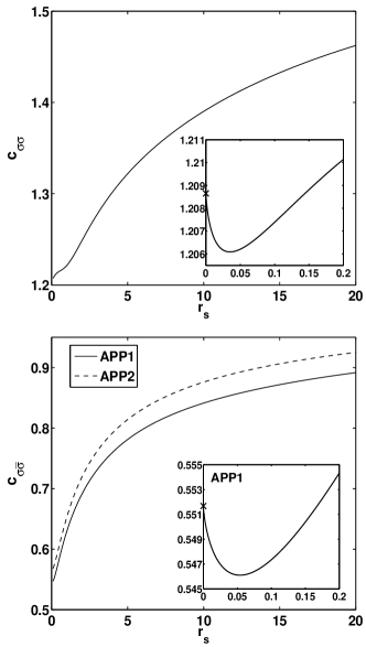
Figure 1: Upper panel: Optimal coefficients $c_{\sigma\sigma}$ for locally reproducing the correlation energy densities of the homogeneous two-dimensional electron gas. The inset show the detailed behavior in the high-density limit $r_{s}\rightarrow 0$. Lower panel: Same for $c_{\sigma\bar{\sigma}}$. Solid and dashed lines correspond to two difference approximations for the polarized component of the correlation energy in the unpolarized electron gas (see text). The inset corresponds to the high-density result in the first approximation (APP1).

for realistic densities ($0<r_{s}<20$). The data could be easily tabulated or parametrized for convenient use of the functional. For this range of densities we may use approximate parametrization of the form

$$c_{\sigma\sigma}[r_{s}]\approx\alpha\,\log(r_{s})+\beta\,r_{s}^{\gamma}$$ (13)

with $\alpha=-0.1415\,1$, $\beta=1.226\,1$, and $\gamma=0.144\,99$. We remind that when using the correlation functional the coefficient $c_{\sigma\sigma}[r_{s}]({\bf r})$ is calculated locally with the local density $r_{s}({\bf r})$.

Let us examine in detail the high-density limit, $r_{s}\rightarrow 0$, for the same-spin coefficient. Expansion of the logarithm in Eq. (12) leads to

$$c_{\sigma\sigma}[r_{s}\rightarrow 0] = \left\{\frac{768}{\pi^{2}(8-3\pi)}\epsilon_{c}^{\rm 2DEG}[r_{s}\rightarrow 0,\zeta=1]\right\}^{1/4}$$ (14)

$$\approx 1.2087,$$

where we have used the known limit for the 2DEG, $\epsilon_{c}^{\rm 2DEG}[r_{s}\rightarrow 0,\zeta=1]\approx-0.039\,075\,0$ (Ref. attaccalite, ). This result coincides with the numerical one in Fig. 1 (see the upper inset). We point out that the “u-shape” at $r_{s}\lesssim 0.05$ is not due to numerical inaccuracies in the present work or in the QMC parametrization, but it arises from the exact properties of the 2DEG correlation energy in the high-density limit. rajagopal

In the low-density limit, $r_{s}\rightarrow\infty$, we obtain from Eq. (12) the leading contribution as

$$c_{\sigma\sigma}[r_{s}\rightarrow\infty] \simeq \left\{\frac{96\,r_{s}}{\pi(8-3\pi)}\epsilon_{c}^{\rm 2DEG}[r_{s}\rightarrow\infty,\zeta=1]\right\}^{1/3}$$ (15)

$$\approx 1.68,$$

where we have used the known result for the 2DEG, $\epsilon_{c}^{\rm 2DEG}[r_{s}\rightarrow\infty,\zeta=1]\rightarrow-0.222/r_{s}$ (Ref. attaccalite, ). From the upper panel of Fig. 1 it is evident that this extreme low-density limit has been not reached yet for $r_{s}\simeq 20$. However, our numerical values at larger $r_{s}$ agree very well with the exact limit.

III.2 Unpolarized case

The coefficient $c_{\sigma{\bar{\sigma}}}[r_{s}]$ can be determined in a similar fashion by employing the results for the correlation energy density of the unpolarized 2DEG, $\epsilon_{c}^{\rm 2DEG}[r_{s},\zeta=0]$. It should be noted that also the same-spin component $U_{c}^{\sigma\sigma}$ depending on the spin density $\rho_{\sigma}$ is needed in the calculation. Now, the fitting to the 2DEG raises the following complication: the parallel-spin contribution of $\epsilon_{c}^{\rm 2DEG}[r_{s},\zeta=0]$, which we here mark as $\epsilon_{c,{\sigma\sigma}}^{\rm 2DEG}[r_{s},\zeta=0]$, is nontrivial; in particular, it is important to note that this contribution is not the same as $\epsilon_{c}^{\rm 2DEG}[r_{s},\zeta=1]$ upon density scaling. In principle, a fully spin-resolved expression is accessible by employing the QMC results for the 2DEG correlation potential energy and using the virial theorem. paola_g For the sake of simplicity, however, we apply here two different approximations for the parallel-spin component. In the first approximation (APP1) we set $\epsilon_{c,{\sigma\sigma}}^{\rm 2DEG}[r_{s},\zeta=0]\approx\epsilon_{c}^{\rm 2DEG}[\sqrt{2}\,r_{s},\zeta=1]$, which is similar to the form of Stoll et al. stoll in 3D electron gas. In fact, this approximation corresponds to the density scaling mentioned above. The second possible approximation (APP2) is given by $\epsilon_{c,{\sigma\sigma}}^{\rm 2DEG}[r_{s},\zeta=0]\approx\epsilon_{c}^{\rm 2DEG}[r_{s},\zeta=1]/\sqrt{2}$, which is similar to the 3D version of Perdew and Wang. pw Even though the first approximation is exact in the limit $r_{s}\rightarrow 0$, the latter type of approximation has been shown to be more accurate gorigiorgi in 3D, and we may thus expect similar tendency in 2D as well. It should be noted, however, that deviations from numerically exact results have been reported in 3D for both approximations, especially at large $r_{s}$ (Ref. paolaperdew, ).

Going back to the determination of $c_{\sigma{\bar{\sigma}}}[r_{s}]$, we consider spin-densities $\rho_{\uparrow}=\rho_{\downarrow}=\rho/2$ and set a condition $U_{c}^{\sigma\sigma}=2\,\epsilon_{c,\sigma\sigma}^{\rm 2DEG}[r_{s},\zeta=0]$ with the approximations APP1 and APP2 for the r.h.s. as specified above. From Eqs. (4)-(6) the formula to be solved for $c_{\sigma{\bar{\sigma}}}[r_{s}]$ is given by

$$\epsilon_{c,\sigma\sigma}^{\rm 2DEG}[r_{s},\zeta=0]-\epsilon_{c}^{\rm 2DEG}[r_{s},\zeta=0]=\frac{(\pi-2)}{4\pi r_{s}^{2}}$$

$$\times\left[\frac{3\pi\sqrt{2}}{4}r_{s}c_{\sigma{\bar{\sigma}}}-\ln\left(1+\frac{3\pi\sqrt{2}}{4}r_{s}c_{\sigma{\bar{\sigma}}}\right)\right].$$ (16)

The result is shown in the lower part of Fig. 1 for both APP1 (solid line) and APP2 (dashed line). Both curves for this density range ($0<r_{s}<20$) can be approximated with a satisfactory accuracy by a simple parametrized formula

$$c_{\sigma{\bar{\sigma}}}[r_{s}]\approx\delta\,r_{s}^{\xi}$$ (17)

with $\delta=0.653\,58$ and $\xi=0.116\,91$ for APP1 and $\delta=0.663\,25$ and $\xi=0.123\,96$ for APP2.

Again, let us consider the high- and low-density limits for the obtained expressions. In the high-density limit we find a semi-analytic expression

$$c_{\sigma{\bar{\sigma}}}[r_{s}\rightarrow 0]=\frac{8}{3\sqrt{\pi(\pi-2)}}\,\bigg{\{}\epsilon_{c,\sigma\sigma}^{\rm 2DEG}[r_{s}\rightarrow 0,\zeta=0]\\ -\epsilon_{c}^{\rm 2DEG}[r_{s}\rightarrow 0,\zeta=0]\bigg{\}}^{1/2}.$$ (18)

Using the known limit $\epsilon_{c}^{\rm 2DEG}[r_{s}\rightarrow 0,\zeta=0]\approx-0.192\,500$ (Ref. attaccalite, ) leads to $c^{\rm APP1}_{\sigma{\bar{\sigma}}}[r_{s}\rightarrow 0]\approx 0.55168$, which corresponds to the exact result in this limit as mentioned above, and $c^{\rm APP2}_{\sigma{\bar{\sigma}}}[r_{s}\rightarrow 0]\approx 0.57175$. Both values coincide with the numerical results in Fig. 1 (see the lower panel for a detailed view on APP1).

In the low-density limit Eq. (III.2) yields

$$c_{\sigma\bar{\sigma}}[r_{s}\rightarrow\infty]=\frac{16\,r_{s}}{3\sqrt{2}(\pi-2)}\bigg{\{}\epsilon_{c,\sigma\sigma}^{\rm 2DEG}[r_{s}\rightarrow\infty,\zeta=0]\\ -\epsilon_{c}^{\rm 2DEG}[r_{s}\rightarrow\infty,\zeta=0]\bigg{\}}$$ (19)

From the knowledge that $\epsilon_{c}^{\rm 2DEG}[r_{s}\rightarrow\infty,\zeta=0]\rightarrow-0.470/r_{s}$ (Ref. attaccalite, ), we obtain $c_{\sigma\bar{\sigma}}[r_{s}\rightarrow\infty]\simeq 1.03$. Note that the limit value is the same for APP1 and APP2, which is obvious due to the low-density decay of the correlation energy as $\propto 1/r_{s}$ in the fully-polarized 2DEG (see the previous section). The congruence in the limit value between APP1 and APP2 is not evident in the density range ($r_{s}\leq 20$) shown in Fig. 1. In fact, the decay towards the same limit can be seen only at very high $r_{s}$ as we have confirmed numerically.

It is reassuring to note that, to the leading order, both high- and low-density limits of our model correlation energies obtained through Eqs. (12) and (III.2) are in agreement with the corresponding exact expansions regarding their functional dependence with respect to the density parameter $r_{s}$. More specifically, $\epsilon_{c}^{\rm 2DEG}[r_{s}\rightarrow 0,\zeta=0]$ and $\epsilon_{c}^{\rm 2DEG}[r_{s}\rightarrow 0,\zeta=1]$ attain a finite ($r_{s}$ independent) value in the high-density limit, while $\epsilon_{c}^{\rm 2DEG}[r_{s}\rightarrow\infty,\zeta=0]$ and $\epsilon_{c}^{\rm 2DEG}[r_{s}\rightarrow\infty,\zeta=1]$ decay as $r_{s}^{-1}$ in the low-density limit.

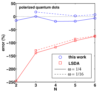
Figure 2: (color online). Relative errors produced by the present functional (circles) and the local spin-density approximation (squares) in correlation energies of spin-polarized quantum dots with respect to numerically accurate results in Ref. rontani, (see text).

IV Testing on inhomogeneous systems

Next we test the functional, i.e., Eqs. (3-9) with the coefficients $c_{\sigma\sigma}$ and $c_{\sigma{\bar{\sigma}}}$ taken from Eqs. (13) and (17), respectively, for a set of 2D parabolic quantum dots, where the external confining potential is given by $v(r)=\omega^{2}r^{2}/2$ with $\omega$ being the confinement strength. The correlation energies obtained from Eq. (5) are compared to the reference results $E_{c}^{\rm ref}=E_{\rm tot}^{\rm ref}-E_{\rm tot}^{\rm EXX}$, where $E_{\rm tot}^{\rm ref}$ is the analytic, taut ED, rontani or QMC, pederiva total energy, and $E_{\rm tot}^{\rm EXX}$ is the exact-exchange (EXX) total energy obtained in the Krieger-Li-Iafrate approximation kli with the octopus code. octopus The EXX result is used as input for our functional, including $U_{x}^{\sigma}$ as the exact exchange-hole potential.

IV.1 Fully-polarized quantum dots

Figure 2 shows the relative errors in the correlation energies for fully-polarized QDs of $N=2\ldots 6$ electrons and confinement strengths $\omega=1/4$ (solid lines) and $\omega=1/16$ (dashed lines). The errors produced by the present functional and by the LSDA with respect to the ED results in Ref. rontani, are presented by circles and squares, respectively. The present functional clearly outperforms the LSDA by reducing the error in the correlation energy by one order of magnitude on the average (mean absolute errors $120\,\%$ and $11\,\%$, respectively). The performance of the present functional is stable regardless of $N$ and $\omega$, whereas the LSDA gains accuracy very slowly as a function of $N$. Since our functional coincides with the LSDA in the 2DEG limit by construction, it can be expected that the error of the present functional diminishes further at larger $N$. This desired tendency is clearly missed if a fixed value for $c_{\sigma\sigma}$ is used. prev

IV.2 Unpolarized quantum dots

In Table 1

Table 1: Comparison of the correlation energies for unpolarized parabolic quantum dots. The reference results have been obtained from numerically accurate data for the total energy (see text). APP1 and APP2 correspond to our functional with two different approximations for the parallel-spin component, respectively (see text). The last row shows the mean absolute error (in percentage), $\Delta=\left<|E_{c}-E_{c}^{\rm ref}|/|E_{c}^{\rm ref}|\right>$.

$N$	$\omega$	$E_{\rm tot}^{\rm ref}$	$E_{\rm c}^{\rm ref}$	$E_{c}^{\rm APP1}$	$E_{c}^{\rm APP2}$	$E_{c}^{\rm LSDA}$
2	1	$3^{*}$	-0.162	-0.144	-0.147	-0.199
2	1/4	$0.9324^{\dagger}$	-0.114	-0.098	-0.101	-0.139
2	1/6	$2/3^{*}$	-0.102	-0.085	-0.087	-0.122
2	1/16	$0.3031^{\dagger}$	-0.070	-0.057	-0.059	-0.085
2	1/36	$0.1607^{\dagger}$	-0.049	-0.040	-0.041	-0.061
6	$1/1.89^{2}$	$7.6001^{\ddagger}$	-0.421	-0.396	-0.405	-0.473
6	1/4	$6.995^{\dagger}$	-0.396	-0.381	-0.390	-0.457
6	1/16	$2.528^{\dagger}$	-0.250	-0.221	-0.228	-0.279
12	$1/1.89^{2}$	$25.636^{\ddagger}$	-0.917	-0.895	-0.915	-1.000
$\Delta$				$11\,\%$	$9\,\%$	$18\,\%$

^∗ Analytic solution by Taut from Ref. taut, . ^† CI data from Ref. rontani, . ^‡ Diffusion QMC data from Ref. pederiva, .

we compare the correlation energies for a set of unpolarized QDs. Also in this case the present functional, with both approximations APP1 and APP2 for the parallel-spin component, is more accurate than the LSDA. As expected, LSDA becomes again more accurate with $N$, but this tendency can be found also in the present functional, where it is in fact significantly stronger than in the LSDA. For example, for $N=2$, $N=6$, and $N=12$ with roughly the same $\omega$, the LSDA yields relative errors of $-22\,\%$, $-12\,\%$, and $-9\,\%$ in the correlation energies, respectively. When using our functional with APP1 the corresponding errors are $14\,\%$, $6\,\%$, and $2\,\%$, respectively, and within APP2 the errors reduce further to $11\,\%$, $1.5\,\%$, and $0.2\,\%$. As can be seen in Ref. prev, , the functional having a fixed value for $c_{\sigma{\bar{\sigma}}}$ is far from this accuracy. The better performance of APP2 in comparison with APP1 is in line with the results for the 3D electron gas, where the approximation of Perdew and Wang pw (similar to APP2) is more accurate than the one by Stoll et al. stoll (similar to APP1).

Before concluding, it is natural to ask if the exchange-hole potential $U_{x}^{\sigma}({\bf r})$ may be treated approximately to reduce the burden of the EXX calculation without losing the accuracy. Possible choices may be the LSDA expression, or the GGA and meta-GGA as given in Refs. gga, ; gamma, ; x1, ; x2, . Also the goal is to carry out fully self-consistent calculations and preferably for a larger variety of 2D systems, e.g., for quantum-ring structures. Here we have focused solely on parabolic QDs representing, through comparison with experimental data, impurity ; spindroplet ; max a valid approximation for both vertical and lateral semiconductor QD devices. The above outlined tasks clearly deserve extended future investigations.

V Conclusion

We have developed a spin-dependent parameter-free density functional to calculate the correlation energies in two-dimensional electron systems. The functional has been constructed through physically reasonable modeling of the angular-averaged, spin-resolved correlation hole functions. The key extension to previous works is enforcing the functional to reproduce the correlation energies of the homogeneous two-dimensional electron gas. We have shown that this is possible by transforming the coefficients – involved in the estimation of the characteristic sizes of the correlation holes – to functionals of the electron density. As a result, we are able to find very accurate correlation energies for quantum dots with varying confinement strength and number of electrons. Most importantly, the significant error reduction as a function of the number of electrons makes the present functional a predictive method to obtain correlation energies of systems which are beyond the capabilities of exact-diagonalization and quantum Monte Carlo techniques.

- (1) For a review, see, e.g., L. P. Kouwenhoven, D. G. Austing, and S. Tarucha, Rep. Prog. Phys. 64 (2001) 701; S. M. Reimann and M. Manninen, Rev. Mod. Phys. 74 (2002) 1283.
- (2) M. Rontani, C. Cavazzoni, D. Bellucci, and G. Goldoni, J. Chem. Phys. 124, 124102 (2006).
- (3) For a review, see, A. Harju, J. Low Temp. Phys. 140, 181 (2005).
- (4) F. Pederiva, C. J. Umrigar, and E. Lipparini, Phys. Rev. B 62, 8120 (2000); ibid 68, 089901 (2003).
- (5) A. D. Güçlü, J.-S. Wang, and H. Guo, Phys. Rev. B 68, 035304 (2003).
- (6) See, e.g., U. De Giovannini, F. Cavaliere, R. Cenni, M. Sassetti, and B. Kramer, Phys. Rev. B 77, 035325 (2008).
- (7) For reviews about DFT, see, e.g., R. M. Dreizler and E. K. U. Gross, Density functional theory (Springer, Berlin, 1990); U. von Barth, Phys. Scr. T109, 9 (2004); J. P. Perdew and S. Kurth, in A Primer in Density Functional Theory (Springer, Berlin, 2003).
- (8) For applications of DFT to quantum dots, see, e.g., Refs. [9-16] and references therein.
- (9) P. Gori-Giorgi, M. Seidl, and G. Vignale, Phys. Rev. Lett. 103 166402 (2009).
- (10) S. Pittalis, E. Räsänen, N. Helbig, and E. K. U. Gross, Phys. Rev. B 76, 235314 (2007).
- (11) E. Räsänen, S. Pittalis, C. R. Proetto, and E. K. U. Gross, Phys. Rev. B 79, 121305(R) (2009).
- (12) S. Pittalis, E. Räsänen, J. G. Vilhena, M. A. L. Marques, Phys. Rev. A 79, 012503 (2009).
- (13) S. Pittalis, E. Räsänen, and E. K. U. Gross, Phys. Rev. A 80, 032515 (2009).
- (14) S. Pittalis, E. Räsänen, C. R. Proetto, and E. K. U. Gross, Phys. Rev. B 79, 085316 (2009).
- (15) S. Pittalis, E. Räsänen, and M. A. L. Marques, Phys. Rev. B 78, 195322 (2008).
- (16) S. Pittalis and E. Räsänen, Phys. Rev. B 80, 165112 (2009).
- (17) S. Pittalis, E. Räsänen, and C. R. Proetto, Phys. Rev. B 81, 115108 (2010).
- (18) A. K. Rajagopal and J. C. Kimball, Phys. Rev. B 15, 2819 (1977).
- (19) C. Attaccalite, S. Moroni, P. Gori-Giorgi, and G. B. Bachelet, Phys. Rev. Lett. 88, 256601 (2002).
- (20) A. D. Becke, J. Chem. Phys. 88, 1053 (1988).
- (21) A. D. Becke, Can. J. Chem. 74, 995 (1996).
- (22) A. D. Becke and M. R. Roussel, Phys. Rev. A 39, 3761 (1989).
- (23) A. D. Becke, J. Chem. Phys. 117, 6935 (2002).
- (24) P. Gori-Giorgi, S. Moroni, and G. B. Bachelet, Phys. Rev. B 70, 115102 (2004).
- (25) H. Stoll, C. M. E. Pavlidou, and H. Preuss, Theor. Chim. Acta 49, 143 (1978).
- (26) J. P. Perdew and Y. Wang, Phys. Rev. B 46, 12 947 (1992).
- (27) P. Gori-Giorgi, F. Sacchetti, and G. B. Bachelet, Phys. Rev. B 61, 7353 (2000).
- (28) P. Gori-Giorgi and J. P. Perdew, Phys. Rev. B 69, 041103(R) (2004).
- (29) M. Taut, J. Phys. A 27, 1045 (1994).
- (30) J. B. Krieger, Y. Li, and G. J. Iafrate, Phys. Rev. A 46, 5453 (1992).
- (31) M. A. L. Marques, A. Castro, G. F. Bertsch and A. Rubio, Comp. Phys. Comm. 151, 60 (2003); A. Castro, H. Appel, M. Oliveira, C. A. Rozzi, X. Andrade, F. Lorenzen, M. A. L. Marques, E. K. U. Gross, and A. Rubio, Phys. Stat. Sol. (b) 243, 2465 (2006).
- (32) E. Räsänen, J. Könemann, R. J. Haug, M. J. Puska, and R. M. Nieminen Phys. Rev. B 70, 115308 (2004).
- (33) E. Räsänen, H. Saarikoski, A. Harju, M. Ciorga, and A. S. Sachrajda Phys. Rev. B 77, 041302(R) (2008).
- (34) M. Rogge, E. Räsänen, and R. J. Haug, submitted, arXiv:1001.5395 (2010).