CT invariant quantum spin Hall effect in a ferromagnetic graphene

Abstract

We predict a quantum spin Hall effect (QSHE) in the ferromagnetic graphene under a magnetic field. Unlike the previous QSHE, this QSHE appears in the absence of any spin-orbit interaction, thus, arrived from a different physical origin. The previous QSHE is protected by the time-reversal (T) invariance. This new QSHE is protected by the CT invariance, where C is the charge conjugation operation. Due to this QSHE, the longitudinal resistance exhibits quantum plateaus. The plateau values are at $1/2$, $1/6$, $3/28$, … , (in the unit of $h/e^{2}$), depending on the filling factors of the spin-up and spin-down carriers. The spin Hall resistance is also investigated and is found to be robust against the disorder.

In the years since the spin Hall effect (SHE) has been discovered, it has generated great interest.ref1 ; ref2 ; ref3 ; ref4 In the SHE, an applied longitudinal charge current or voltage bias induces a transverse spin current due to the spin-dependent scatteringsref1 ; ref2 of the spin-orbit interaction (SOI)ref3 . Soon afterwards, the quantum SHE (QSHE) is also predicted.ref5 ; ref6 The QSHE occurs in a topological insulator in which the bulk material is an insulator with two helical edge states carrying the current.ref7 The edge states, with opposite spins on a given edge or opposite edges for a given spin direction containing opposite propagation directions, lead to a quantized spin Hall conductance. The QSHE is a new quantum state of matter with a non-trivial topological property. The existence of QSHE was first proposed in a graphene film in which the SOI opened a band gap and established the edge states.ref5 ; ref6 But the sequent work found that the SOI in the graphene was quite weak and the gap-opening was small, so the QSHE was difficult to observe.ref8 Soon afterwards, the QSHE was also predicted to exist in some other systems.ref9 ; ref10 ; ref11 ; ref12 Recently, the QSHE was successfully realized in the CdTe/HgTe/CdTe quantum wells, and a quantized longitudinal resistance plateau was experimentally observed due to the QSHE.ref11

Another subject that has also been extensively investigated in recent years is the graphene, a single-layer hexagonal lattice of carbon atomsref13 after it has been successfully fabricated.ref14 ; ref15 The graphene has a unique band structure with a linear dispersion near the Fermi surface, giving it many peculiar properties. For example, the quasi-particles obey the Dirac-like equation and have relativistic-like behaviors, and its Hall plateaus are at the half-integer values.

In this Letter, we predict a new kind of QSHE in a ferromagnetic graphene. Let us first imagine a two-dimensional system consisting of the following characteristics: (i) its carriers contain electrons and holes; (ii) both electrons and holes are completely spin-polarized with opposite spin polarizations. When a high perpendicular magnetic field is applied to the system, the edge states are formed and the carriers move only along the edges. In particular, the electrons (with their spins up) and holes (with their spins down) move in opposite directions on a given edge (see the inset in Fig.1a). Therefore, the QSHE automatically exists in this system. Although the ordinary metals (or doped semiconductors) cannot meet the above two characteristics, a ferromagnetic graphene does. Recently, several approaches to realize a ferromagnetic graphene have been suggested.ref16 ; ref17 ; ref18 For example, the ferromagnetic graphene can be realized by growing the graphene on a ferromagnetic insulator (e.g. EuO).ref17 For a ferromagnetic graphene, as soon as the Fermi energy $E_{F}$ is tuned to lie between the spin-up and spin-down Dirac points (see the inset in Fig.1b), the above two characteristics are met and the QSHE occurs. In the following calculations, we consider four- and six-terminal graphene Hall bars (see the insets in Fig.1a). The results reveal that the transverse spin current and spin Hall resistance indeed show the quantized plateaus because of the QSHE.

Comparing this new QSHE with the previously-studied QSHE, there are two essential differences: (i) The previous QSHE comes from the SOI and the proposed systems all contain the time-reversal symmetry,ref5 ; ref6 ; ref7 ; ref9 ; ref10 while the present QSHE exists without the SOI and breaks the time-reversal symmetry. However, this new QSHE is protected by CT invariance. (ii) In the previous QSHE, the edge states only carry a spin current while at equilibrium; in this QSHE system, the edge states carry both spin and charge currents at equilibrium with the two edges states being CT partners of each other (see the inset in Fig.1a). Thus, this is a new kind of QSHE and the system is a new type of topological insulator. Due to the topological invariance, the plateaus of the spin Hall resistance are robust to disorder or impurity scattering. So the plateau is very stable and its value can be used as the standard value for the spin Hall resistance.

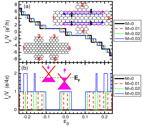
Figure 1: (Color online) The Hall conductance $I_{e}/V$ (a) and spin Hall conductance $I_{s}/V$ (b) vs. the energy $\epsilon_{0}$ for $N=80$ and $\phi=0.005$. The two insets in (a) are the schematic diagram for the four- and six-terminal graphene’s Hall bars. The inset in (b) is the schematic diagram for band structure of the ferromagnetic graphene while $\epsilon_{0}+M>E_{F}>\epsilon_{0}-M$.

In the tight-binding representation, the four- or six-terminal ferromagnetic graphene device (see the insets in Fig.1a) can be described by the Hamiltonian:ref19

$$H=\sum_{i,\sigma}(\epsilon_{0}-\sigma M)a^{\dagger}_{i\sigma}a_{i\sigma}-\sum_{<ij>,\sigma}te^{i\phi_{ij}}a_{i\sigma}^{\dagger}a_{j\sigma},$$ (1)

where $a_{i\sigma}$ and $a_{i\sigma}^{\dagger}$ are the annihilation and creation operators at the discrete site $i$. $\epsilon_{0}$ is the on-site energy (i.e. the Dirac-point energy), $M$ is the ferromagnetic exchange splitref17 , and $t$ is the nearest neighbor hopping element. Here, the whole device, including the center region and four or six terminals, is made of the ferromagnetic graphene. With the presence of a perpendicular magnetic field $B$, a phase factor $\phi_{ij}$ is added to the hopping element, $\phi_{ij}=\int_{i}^{j}\vec{A}\cdot d\vec{l}/\phi_{0}$ with the vector potential $\vec{A}=(-By,0,0)$ and $\phi_{0}=\hbar/e$.

The transmission coefficient $T_{pq\sigma}(\epsilon)$ from the terminal $q$ to the terminal $p$ with spin $\sigma$ can be calculated from the equation:ref20 $T_{pq\sigma}(\epsilon)=Tr[{\bf\Gamma}_{p\sigma}{\bf G}_{\sigma}^{r}{\bf\Gamma}_{q\sigma}{\bf G}^{a}_{\sigma}]$, where ${\bf\Gamma}_{p\sigma}(\epsilon)=i[{\bf\Sigma}^{r}_{p\sigma}(\epsilon)-{\bf\Sigma}^{a}_{p\sigma}(\epsilon)]$, the Green functions ${\bf G}^{r}_{\sigma}(\epsilon)=[{\bf G}^{a}_{\sigma}(\epsilon)]^{\dagger}=1/[\epsilon-{\bf H}^{cen}_{\sigma}-\sum_{p}{\bf\Sigma}^{r}_{p\sigma}]$, and ${\bf H}^{cen}_{\sigma}$ is the Hamiltonian of the center region. The retarded self-energy ${\bf\Sigma}^{r}_{p\sigma}(\epsilon)$ due to the coupling to the terminal $p$ can be calculated numerically.ref21 After obtaining the transmission coefficient, the particle current in the terminal $p$ with the spin ${\sigma}$ can be calculated from the Landauer-B$\ddot{u}$ttiker formula: $I_{p\sigma}=(1/h)\int d\epsilon\sum_{q}T_{pq\sigma}(\epsilon)[f_{q\sigma}(\epsilon)-f_{p\sigma}(\epsilon)]$, where $f_{p\sigma}(\epsilon)=1/\{\exp[(\epsilon-\mu_{p\sigma})/k_{B}T]+1\}$ is the Fermi distribution function in the terminal $p$, with the spin-dependent chemical potential $\mu_{p\sigma}$ and the temperature $T$. In the following numerical calculations, we take $t=1$ as the energy unit and only consider the zero temperature case ($T=0$), as the thermal energy $k_{B}T$ is normally much smaller than other energy scales in the problem. The sample width is denoted by $N$, and the insets of Fig.1a show a system with $N=3$. In the calculations, we choose $N=80$ and $40$, and the corresponding widths are $33.9nm$ and $16.9nm$. The magnetic field is described by the $\phi$ with $\phi\equiv(3\sqrt{3}/4)a^{2}B/\phi_{0}$ and the magnetic flux in a honeycomb lattice is $2\phi$.

We first consider the four-terminal device (see the inset at the top right corner of Fig.1a) and a small bias $V$ is applied between the longitudinal terminals 1 and 3 to study the induced charge current $I_{ne}$ [$I_{ne}\equiv e(I_{n\uparrow}+I_{n\downarrow})$] and spin current $I_{ns}$ [$I_{ns}\equiv(\hbar/2)(I_{n\uparrow}-I_{n\downarrow})$] in the transversal terminals 2 and 4. Here the boundary conditions for the four terminals are $\mu_{1\uparrow}=\mu_{1\downarrow}=eV/2$, $\mu_{2\uparrow}=\mu_{2\downarrow}=0$, $\mu_{3\uparrow}=\mu_{3\downarrow}=-eV/2$, and $\mu_{4\uparrow}=\mu_{4\downarrow}=0$. The currents in the terminals 2 and 4 satisfy the relations: $I_{2e}=-I_{4e}\equiv I_{e}$ and $I_{2s}=-I_{4s}\equiv I_{s}$. Fig.1a and 1b show the Hall conductance $I_{e}/V$ and spin Hall conductance $I_{s}/V$ versus the Dirac-point energy $\epsilon_{0}$, respectively. For a non-ferromagnetic graphene ($M=0$) under the high magnetic field ($\phi=0.005$), $I_{s}/V$ is zero and $I_{e}/V$ exhibits the plateaus at odd integer values $ne^{2}/h$ ($n=\pm 1$, $\pm 3$, …) due to the quantum Hall effect (QHE). These results have been observed in recent experiments.ref14 ; ref15 For a ferromagnetic graphene with $M\not=0$, the spin current emerges (see Fig.1b) since the QSHE. The spin Hall conductance $I_{s}/V$ also shows the quantized plateaus. By considering the edge state under the high magnetic field, the plateau values of $I_{s}/V$ and $I_{e}/V$ can be analytically derived to be at $(\nu_{\uparrow}-\nu_{\downarrow})e/8\pi$ and $(\nu_{\uparrow}+\nu_{\downarrow})e^{2}/2h$,supplement where $\nu_{\sigma}$ is the Landau filling factor for spin $\sigma$. In particular, when $|\epsilon_{0}|<|M|$, in which case the Fermi energy $E_{F}$ ($E_{F}=0$) is located between the spin-up Dirac-point $\epsilon_{0}-M$ and the spin-down Dirac-point $\epsilon_{0}+M$, $I_{e}$ is zero and a net quantum spin current emerges in the transversal terminals. In addition, if in the open circuit case, the spin accumulation emerges at the sample boundaries instead of the spin current.supplement

Since the QSHE can give rise to quantum plateaus in resistances, we next study the longitudinal and Hall resistances in the six-terminal Hall device (see the inset in the lower left corner of Fig.1a). Now we consider a small bias $V$ applied to the longitudinal terminals 1 and 4. The transversal terminals 2, 3, 5, and 6 are all voltage probes, their charge currents vanish ($I_{pe}=0$) and $\mu_{p\uparrow}=\mu_{p\downarrow}\equiv\mu_{p}$. Combining these boundary conditions with the Landauer-B$\ddot{u}$ttiker formula, the voltages $V_{p}$ ($V_{p}=\mu_{p}/e$) in four voltage probes can be obtained, then the longitudinal resistance $R_{14,23}=(V_{2}-V_{3})/I_{14}$ and Hall resistance $R_{14,26}=(V_{2}-V_{6})/I_{14}$ are calculated, here $I_{14}=-I_{1e}=I_{4e}$. The resistances contain the properties $R_{14,26}=R_{14,35}$ and $R_{14,23}=R_{14,65}$.

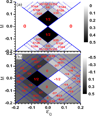
Figure 2: The panels (a) and (b) show the resistances $R_{14,23}$ and $R_{14,26}$ (in the unit of $h/e^{2}$) vs the exchange split $M$ and energy $\epsilon_{0}$ for $N=80$ and $\phi=0.005$.

Fig.2a and 2b show the longitudinal and Hall resistances, $R_{14,23}$ and $R_{14,26}$, versus the energy $\epsilon_{0}$ and the exchange split $M$ at an external magnetic field $\phi=0.005$. Due to the QSHE and QHE, both $R_{14,23}$ and $R_{14,26}$ may be non-zero, and they both exhibit plateau structures. The plateau values are determined by the filling factors $\nu_{\uparrow}$ and $\nu_{\downarrow}$. For the fixed filling factors $\nu_{\uparrow}$ and $\nu_{\downarrow}$, $R_{14,23}$ and $R_{14,26}$ maintain their plateau values regardless of $\epsilon_{0}$ and $M$. By considering the carriers transport along the edge states, the plateau values can be analytically derived:supplement $R_{14,23}=0$ and $R_{14,26}=[1/(\nu_{\uparrow}+\nu_{\downarrow})]h/e^{2}$ for $(\nu_{\uparrow},\nu_{\downarrow})=(+,+)$ or $(-,-)$, and $R_{14,23}=[|\nu_{\uparrow}\nu_{\downarrow}|/(|\nu_{\uparrow}|^{3}+|\nu_{\downarrow}|^{3})]h/e^{2}$ and $R_{14,26}=sign(\nu_{\uparrow})[(|\nu_{\uparrow}|^{2}-|\nu_{\downarrow}|^{2})/(|\nu_{\uparrow}|^{3}+|\nu_{\downarrow}|^{3})]h/e^{2}$ for $(\nu_{\uparrow},\nu_{\downarrow})=(+,-)$ or $(-,+)$. Some plateau values for low $\nu_{\uparrow},\nu_{\downarrow}$ have been labeled in Fig.2. The numerical results in Fig.2 are in excellent agreement with the analytic plateau values (the differences between them are less than $10^{-6}$). Furthermore, $R_{14,23}$ and $R_{14,26}$ have the following properties: While $|\epsilon_{0}|>|M|$ with $(\nu_{\uparrow},\nu_{\downarrow})=(+,+)$ or $(-,-)$, the longitudinal resistance $R_{14,23}$ is zero and only the Hall resistance $R_{14,26}$ exists because the spin-up and spin-down carriers are simultaneously either electron-like or hole-like and move in the same direction. On the other hand, while $|\epsilon_{0}|<|M|$ with $(\nu_{\uparrow},\nu_{\downarrow})=(+,-)$ or $(-,+)$, the Fermi energy $E_{F}$ is located between $\epsilon_{0}+M$ and $\epsilon_{0}-M$, the longitudinal resistance $R_{14,23}$ emerges since now the spin-up and spin-down carriers move in opposite directions for a given edge. (i) While $\nu_{\uparrow}=-\nu_{\downarrow}\equiv\nu$, the Hall resistance $R_{14,26}=0$, only the longitudinal resistance $R_{14,23}$ exists with the value $(1/2\nu)h/e^{2}$. This means that only the QSHE emerges and the QHE vanishes in this region. In this case, the system has the CT invariance. Furthermore, if $\nu_{\uparrow}=-\nu_{\downarrow}=\pm 1$, $R_{14,26}=0$ and $R_{14,23}=(1/2)(h/e^{2})$. Now the observed phenomena are completely the same with the QSHE from the SOI,ref5 ; ref6 ; ref7 ; ref9 ; ref10 but their physical mechanisms are different. (ii) While $\nu_{\uparrow}\not=-\nu_{\downarrow}$ but still with ($\nu_{\uparrow}$, $\nu_{\downarrow})=(+,-)$ or $(-,+)$, $R_{14,26}$ is now non-zero since the numbers of the spin-up and spin-down edge states are different. In this case, both resistances $R_{14,26}$ and $R_{14,23}$ have non-zero quantized plateaus and the QSHE and QHE coexist. Fig.3 shows the resistances $R_{14,23}$ and $R_{14,26}$ versus the energy $\epsilon_{0}$ for a fixed $M$ (i.e. along the horizontal lines in Fig.2), and it clearly shows that the quantum plateaus persist very well.

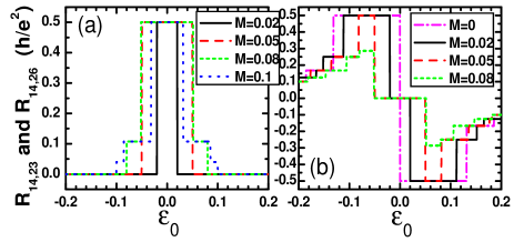
Figure 3: (Color online) The resistances $R_{14,23}$ (a) and $R_{14,26}$ (b) vs the energy $\epsilon_{0}$ for $N=80$ and $\phi=0.005$.

Up to now, we demonstrate the existence of QSHE in the ferromagnetic graphene from both physical picture and detailed numerical calculations. In the following, we study the properties of the spin Hall resistance $R_{s}$, a measurable quantity robust to dephasingref22 and well reflecting the topological invariance of the system. We again consider the four-terminal Hall bar. But now the transversal terminals 2 and 4 are spin-biased probes with boundary conditions $I_{p\uparrow}=I_{p\downarrow}=0$ ($p=2,4$). Here the spin Hall resistance $R_{s}$ is defined as the transversal spin bias over the longitudinal charge current: $R_{s}\equiv(\mu_{2\uparrow}-\mu_{2\downarrow})/eI_{13}=-(\mu_{4\uparrow}-\mu_{4\downarrow})/eI_{13}$. Since the spin bias $\mu_{n\uparrow}-\mu_{n\downarrow}$ is experimentally measurable, so is the $R_{s}$.ref23 ; ref24 Fig.4 shows $R_{s}$ versus the energy $\epsilon_{0}$ for different ferromagnetic exchange split $M$ and magnetic field $\phi$. For $|\epsilon_{0}|>|M|$ with $(\nu_{\uparrow},\nu_{\downarrow})=(+,+)$ or $(-,-)$, $R_{s}=0$. On the other hand, while $|\epsilon_{0}|<|M|$ with $(\nu_{\uparrow},\nu_{\downarrow})=(+,-)$ or $(-,+)$, $R_{s}$ exists. $R_{s}$ exhibits the quantum plateaus, and its plateau values are at $[1/(|\nu_{\uparrow}|+|\nu_{\downarrow}|)]h/e^{2}$. For a small $M$ (e.g. $M=0.02t$ or $0.05t$ in Fig.4b) or a high magnetic field $\phi$ (e.g. $\phi=0.005$ in Fig.4a), $(\nu_{\uparrow},\nu_{\downarrow})$ can only equal to $(1,-1)$, so only the plateau of $R_{s}=h/2e^{2}$ emerges. But for a large $M$ or a small magnetic field $\phi$, $(\nu_{\uparrow},\nu_{\downarrow})$ may be $(1,-3)$, $(3,-1)$, $(1,-5)$, $(5,-1)$, etc, then the plateaus of $R_{s}=h/4e^{2}$, $h/6e^{2}$, etc, are also possible.

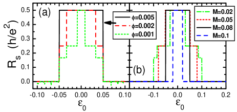
Figure 4: (Color online) (a) shows $R_{s}$ vs $\epsilon_{0}$ for $M=0.05$ and (b) shows $R_{s}$ vs $\epsilon_{0}$ for $\phi=0.005$. The parameter $N=80$.

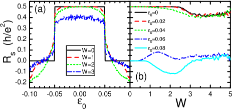
Figure 5: (Color online) $R_{s}$ vs $\epsilon_{0}$ (a) and $R_{s}$ vs the disorder strength $W$ (b) with the parameters $N=40$, $\phi=0.007$, and $M=0.05$. The curves in (a) and (b) are averaged over up to 1000 and 8000 random configurations, respectively.

Finally, we examine the disorder effect on the spin Hall resistance $R_{s}$. Here we assume that the disorder only exists in the central region (see dotted box in top right inset of Fig.1a). Due to the disorder, the on-site energy $\epsilon_{0}-\sigma M$ for each site $i$ in the central region is changed to $\epsilon_{0}+w_{i}-\sigma M$, where $w_{i}$ is uniformly distributed in the range $[-W/2,W/2]$ with the disorder strength $W$. Fig.5a shows $R_{s}$ versus the energy $\epsilon_{0}$ at the different disorder strengths $W$ and Fig.5b shows $R_{s}$ versus the disorder strength $W$ at different energies $\epsilon_{0}$. The results show that the quantum plateaus of $R_{s}$ are very robust against the disorder because of the topological invariance of the system. The quantum plateau maintains its quantized value very well even when $W$ reaches 2 (see Fig.5a and 5b). Since the plateau is so robust and stable, its value can be used as the standard for the spin Hall resistance. In addition, even for a very large disorder strength $W$ (e.g. $W=5$ or larger), the plateau value only slightly decreases while maintaining the plateau structure (see Fig.5b). This is because although the disorder strongly weakens the spin bias $\mu_{2\uparrow}-\mu_{2\downarrow}$, it also weakens the longitudinal charge current $I_{13}$, so the value of $R_{s}$ is affected less. This means that in the large disorder limits ($W\rightarrow\infty$), although the QSHE is broken, the SHE still holds.

In summary, we predict a new QSHE in the ferromagnetic graphene film. Unlike the QSHEs studied so far, the origin of this QSHE is not caused by the spin-orbit interaction. The results also show that the system can exhibit the QSHE, the QHE, and the coexistence of the QSHE and QHE, depending on the filling factors of the spin-up and spin-down carriers. Due to the QSHE and QHE, both the longitudinal and Hall resistances exhibit the plateau structures. The plateau values (in the unit of $h/e^{2}$) are at $1/2$, $1/6$, $3/28$, …, for the longitudinal resistance and at $\pm 1/2$, $\pm 1/4$, $\pm 1/6$, $\pm 2/7$, …, for the Hall resistance. In addition, the spin Hall resistance has also investigated and found to be robust against the disorder.

Acknowledgments: This work was financially supported by NSF-China under Grants Nos. 10525418, 10734110, and 10821403, China-973 program and US-DOE under Grants No. DE-FG02- 04ER46124. Q.F.S. gratefully acknowledges Prof. R. B. Tao for many helpful discussions.

References

- (1) Electronic address: sunqf@aphy.iphy.ac.cn
- (2) M.I. Dyakonov and V.I. Perel, JETP Lett. 13, 467 (1971).
- (3) J.E. Hirsch, Phys. Rev. Lett. 83, 1834 (1999).
- (4) S. Murakami, N. Nagaosa and, S.C. Zhang, Science 301, 1348 (2003); J. Sinova et al., Phys. Rev. Lett. 92, 126603 (2004).
- (5) Y.K. Kato et al., Science 306, 1910 (2004); J. Wunderlich et al., Phys. Rev. Lett. 94, 047204 (2005).
- (6) C.L. Kane, E.J. Mele, Phys. Rev. Lett 95, 146802(2005).
- (7) C.L. Kane, E.J. Mele, Phys. Rev. Lett 95, 226801(2005).
- (8) C. Day, Physics Today 61 19 (2008); N. Nagaosa, Science 318, 758 (2007).
- (9) H. Min et al., Phys. Rev. B 74, 165310 (2006); Y. Yao et al., Phys. Rev. B 75, 041401(R) (2007).
- (10) L. Sheng, et al., Phys. Rev. Lett 95, 136602 (2005); B.A. Bernevig and S.-C. Zhang, Phys. Rev. Lett 96, 106802 (2006); L. Fu, C.L. Kane, and E.J. Mele, Phys. Rev. Lett 98, 106803 (2007); C. Liu, et al., Phys. Rev. Lett 100, 236601 (2008).
- (11) B.A. Bernevig, T.L. Hughes and S.C. Zhang, Science 314, 1757 (2006).
- (12) M. Knig, et al., Science 318, 766 (2007).
- (13) D. Hsieh, et al., Nature (London) 452, 970 (2008).
- (14) C.W.J. Beenakker, Rev. Mod. Phys. 80, 1337 (2008); A.H. Castro Neto, et al., Rev. Mod. Phys. 81, 109 (2009).
- (15) K.S. Novoselov, et al., Science 306, 666 (2004); Nature (London) 438, 197 (2005); Nat. Phys. 2, 177 (2006).
- (16) Y. Zhang, et al., Nature (London) 438, 201 (2005).
- (17) Y.-W. Son et al., Nature (London) 444, 347 (2006); E.-J. Kan et al., Appl. Phys. Lett. 91, 243116 (2007).
- (18) H. Haugen et al., Phys. Rev. B 77, 115406 2008; J. Linder et al., Phys. Rev. Lett. 100, 187004 (2008).
- (19) Q. Zhang et al., Phys. Rev. Lett. 101, 047005 (2008).
- (20) W. Long, Q.F. Sun, and J. Wang, Phys. Rev. Lett. 101, 166806 (2008).
- (21) Electronic Transport in Mesoscopic Systems, edited by S. Datta (Cambridge University Press 1995).
- (22) D.H. Lee and J.D. Joannopoulos, Phys. Rev. B 23, 4997 (1981); M.P. Lopez Sancho, et al., J. Phys. F: Met. Phys. 14, 1205 (1984); 15, 851 (1985).
- (23) See EPAPS Document No. E-PRLTAO-***-****** for supplementary material. For more information on EPAPS, see http://www.aip.org/pubservs/epaps.html.
- (24) H. Jiang et al., Phys. Rev. Lett. 103, 036803 (2009).
- (25) E.J. Koop, et al., Phys. Rev. Lett. 101, 056602 (2008); Q.-F. Sun, et al., Phys. Rev. B 77, 195313 (2008); Y.X. Xing, et al., Appl. Phys. Lett. 93, 142107 (2008).
- (26) S.M. Frolov, et al., Phys. Rev. Lett. 102, 116802 (2009); Nature 458, 868 (2009).