Dark matter halos in the standard cosmological model: results from the Bolshoi simulation
Abstract
Lambda Cold Dark Matter (CDM) is now the standard theory of structure formation in the Universe. We present the first results from the new Bolshoi dissipationless cosmological CDM simulation that uses cosmological parameters favored by current observations. The Bolshoi simulation was run in a volume 250 Mpc on a side using 8 billion particles with mass and force resolution adequate to follow subhalos down to the completeness limit of km s-1 maximum circular velocity. Using merger trees derived from analysis of 180 stored time-steps we find the circular velocities of satellites before they fall into their host halos. Using excellent statistics of halos and subhalos (10 million at every moment and 50 million over the whole history) we present accurate approximations for statistics such as the halo mass function, the concentrations for distinct halos and subhalos, abundance of halos as a function of their circular velocity, the abundance and the spatial distribution of subhalos. We find that at high redshifts the concentration falls to a minimum value of about 4.0 and then rises for higher values of halo mass, a new result. We present approximations for the velocity and mass functions of distinct halos as a function of redshift. We find that while the Sheth-Tormen approximation for the mass function of halos found by spherical overdensity is quite accurate at low redshifts, the ST formula over-predicts the abundance of halos by nearly an order of magnitude by . We find that the number of subhalos scales with the circular velocity of the host halo as , and that subhalos have nearly the same radial distribution as dark matter particles at radii 0.3-2 times the host halo virial radius. The subhalo velocity function scales as . Combining the results of Bolshoi and Via Lactea-II simulations, we find that inside the virial radius of halos with the number of satellites is for satellite circular velocities in the range .
1 Introduction
The Lambda Cold Dark Matter (CDM) model is the standard modern theoretical framework for understanding the formation of structure in the universe (Dunkley et al., 2009). With initial conditions consisting of a nearly scale-free spectrum of Gaussian fluctuations as predicted by cosmic inflation, and with cosmological parameters determined from observations, CDM makes detailed predictions for the hierarchical gravitational growth of structure. For the past several years, the best large simulation for comparison with galaxy surveys has been the Millennium Simulation (Springel et al., 2005, MS-I). Here we present the first results from a new large cosmological simulation, which we are calling the Bolshoi simulation (“Bolshoi” is the Russian word for “big”111“Bolshoi” can be translated as (1) big or large (2) great (3) important (4) grown-up. The Bolshoi Ballet performs in Bolshoi Theater in Moscow. ). Bolshoi has nearly an order of magnitude better mass and force resolution than the Millennium Run. The Millennium Run used the first-year (WMAP1) cosmological parameters from the Wilkinson Microwave Anisotropy Probe satellite (Spergel et al., 2003). These parameters are now known to be inconsistent with modern measurements of the cosmological parameters. The Bolshoi simulation used the latest WMAP5 (Hinshaw et al., 2009; Komatsu et al., 2009; Dunkley et al., 2009) and WMAP7 (Jarosik et al., 2010) parameters, which are also consistent with other recent observational data.
The invention of Cold Dark Matter (Primack & Blumenthal, 1984; Blumenthal et al., 1984) soon led to the first CDM -body cosmological simulations (Melott et al., 1983; Davis et al., 1985). Ever since then, such simulations have been essential in order to calculate the predictions of CDM on scales where structure has formed, since the nonlinear processes of structure formation cannot be fully described by analytic calculations. For example, one of the first large simulations of the CDM cosmology (Klypin et al., 1996) showed that the dark matter autocorrelation function is much larger than the observed galaxy autocorrelation function on scales of Mpc, so “scale-dependent anti-biasing” was required for CDM to match the observed distribution of galaxies. Subsequent simulations with resolution adequate to identify the dark matter halos that host galaxies (Jenkins et al., 1998; Colín et al., 1999) demonstrated that the required destruction of dark matter halos in dense regions does indeed occur.
-body simulations have been essential for determining the properties of dark matter halos. It turned out that dark matter halos of all masses typically have a similar radial profile, which can be approximated by the NFW profile (Navarro et al., 1996). Simulations were also crucial for determining the dependence of halo concentration and halo shape on halo mass and redshift (Bullock et al., 2001; Zhao et al., 2003; Allgood et al., 2006; Neto et al., 2007; Macciò et al., 2008), and also for determining the dependence of the concentration of halos on their mass accretion history (Wechsler et al., 2002; Zhao et al., 2009). Here is the virial radius and is the characteristic radius where the log-log slope of the density is equal to . Details are given in §3 and in Appendix B.
One of the main goals of this paper is to provide the basic statistics of halos selected by the maximum circular velocity () of each halo. There are advantages to using the maximum circular velocity as compared with the virial mass. The virial mass is a well defined quantity for distinct halos (those that are not subhalos), but it is ambiguous for subhalos. It strongly depends on how a particular halofinder defines the truncation radius and removes unbound particles. It also depends on the distance to the center of the host halo because of tidal stripping. Instead, the circular velocity is less prone to those complications. Even for distinct halos the virial mass is an inconvenient property because there are different definitions of “virial mass”. None of them is better than the other and different research groups prefer to use their own definition. This causes confusion in the community and makes comparison of results less accurate. The main motivation for using is that it is more closely related to the properties of the central regions of halos and, thus, to galaxies hosted by those halos. For example, for a Milky-Way type halo the radius of the maximum circular velocity is about 40 kpc (and the circular velocity is nearly the same at 20 kpc), while the virial radius is about 300 kpc. As an indication that circular velocities are a better quantity for describing halos, we find that most statistics look very simple when we use circular velocities: they are either pure power-laws (abundance of subhalos inside distinct halos) or power-laws with nearly exponential cutoffs (abundance of distinct halos).
| Hubble | tilt | ref. | |||
|---|---|---|---|---|---|
| WMAP5 | Dunkley et al. (2009) | ||||
| WMAP5+BAO+SN | Dunkley et al. (2009) | ||||
| X-ray clusters | (0.95) | Vikhlinin et al. (2009) | |||
| aaSystematic error | |||||
| X-ray clusters+WMAP5 | (0.719) | (0.963) | Henry et al. (2009) | ||
| X-ray clusters+WMAP5 | (0.95) | Mantz et al. (2008) | |||
| +SN+BAO | |||||
| maxBCG + WMAP5 | (0.70) | (0.96) | Rozo et al. (2009) | ||
| WMAP7+BAO+H0 | Jarosik et al. (2010) | ||||
| Bolshoi simulation | 0.70 | 0.270 | 0.95 | 0.82 | – |
| Millennium simulations | 0.73 | 0.250 | 1.00 | 0.90 | Springel et al. (2005) |
| Via Lactea-II simulation | 0.73 | 0.238 | 0.951 | 0.74 | Diemand et al. (2008) |
Note. — Values in parentheses are priors
This paper is organized as follows. In §2 we give the essential features of the Bolshoi simulation. Section 3 describes the halo identification algorithm used in our analysis. In §4 we present results on masses and concentrations of distinct halos. Here we also present relations between and . The halo velocity function is presented in §5. Estimates of the Tully-Fisher relation are given in Trujillo-Gomez et al. (2010), where we present detailed discussions of numerous issues related with the procedure of assigning luminosities to halos in simulations and confront results with the observed galaxy distribution. In §6 we give statistics of the abundance of subhalos. The number density profiles of subhalos are presented in §7. Section §8 gives a short summary of our results. Appendix A describes details of the halo identification procedure. Appendix B collects useful approximation formulas. Appendix C compares masses of halos found with two different halo-finders: the friends-of-friends algorithm and the spherical overdensity halo-finder used in this paper.
2 Cosmological parameters and Simulations
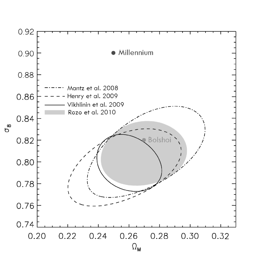
The Bolshoi simulation was run with the cosmological parameters listed in Table 1, together with , . As Table 1 shows, these parameters are compatible with the WMAP seven-year data (WMAP7) (Jarosik et al., 2010) results, with the WMAP five-year data (WMAP5), with WMAP5 combined with Baryon Acoustic Oscillations and Supernova data (Hinshaw et al., 2009; Komatsu et al., 2009; Dunkley et al., 2009). The parameters used for the Bolshoi simulation are also compatible with the recent constraints from the Chandra X-ray cluster cosmology project (Vikhlinin et al., 2009) and other recent X-ray cluster studies. The Bolshoi parameters are in excellent agreement with the SDSS maxBCG+WMAP5 cosmological parameters (Rozo et al., 2009). The optical cluster abundance and weak gravitational lensing mass measurements of the SDSS maxBCG cluster catalog are fully consistent with the WMAP5 data, and the joint maxBCG+WMAP5 analysis quoted in Table 1 reduces the errors. Figure 1 shows current observational constraints on the and parameters. It shows graphically that Bolshoi agrees with the recent constraints while Millennium is far outside them.
The Millennium simulation (Springel et al., 2005, MS-I) has been the basis for many studies of the distribution and statistical properties of dark matter halos and for semi-analytic models of the evolving galaxy population. However, it is important to appreciate that this simulation and the more recent Millennium-II simulation (Boylan-Kolchin et al., 2009, MS-II) used the first-year (WMAP1) cosmological parameters, which are rather different from the current parameters summarized in Table 1. The main difference is that the Millennium simulations used a substantially larger amplitude of perturbations than Bolshoi. Formally, the value of used in the Millennium simulations is more than 3 away from the WMAP5+BAO+SN value and nearly 4 away from the WMAP7+BAO+H0 value. However, the difference is even larger on galaxy scales because the Millennium simulations also used a larger tilt for the power spectrum. Figure 2 shows the linear power spectra of the Bolshoi and Millennium simulations. Because of the large difference in the amplitude, it is not surprising that the Millennium simulations over-predict the abundance of galaxy-size halos. The Sheth-Tormen approximation (Sheth & Tormen, 2002) gives a factor of 1.3-1.7 more halos at for Millennium as compared with Bolshoi, which is a large difference. Angulo & White (2009) argue that cosmological N-body simulations can be re-scaled by certain approximations or by other means. However, the accuracy of those re-scalings cannot be estimated without running accurate simulations and testing particular characteristics.

| Parameter | Value |
| Box size ( Mpc) | 250 |
| Number of particles | |
| Mass resolution () | |
| Force resolution | |
| (kpc, physical) | 1.0 |
| Initial redshift | 80 |
| Zero-level mesh | |
| Maximum number of | |
| refinement levels | 10 |
| Zero-level time-step | |
| Maximum number of time-steps | |
| Maximum displacement | 0.10 |
| per time-step | (cell units) |
The Bolshoi simulation uses a computational box across and 8 billion particles, which gives a mass resolution (one particle mass) of . The force resolution (smallest cell size) is physical (proper) 1 kpc (see below for details). For comparison, the Millennium-I simulation had force resolution (Plummer softening length) 5 kpc and the Millennium-II simulation had 1 kpc. Table 2 gives a short summary of various numerical parameters of the Bolshoi simulation.
The Bolshoi simulation was performed with the Adaptive-Refinement-Tree (ART) code, which is an Adaptive-Mesh-Refinement (AMR) type code. A detailed description of the code is given in Kravtsov et al. (1997) and Kravtsov (1999). The code was parallelized using MPI libraries and OpenMP directives (Gottloeber & Klypin, 2008). Details of the time-stepping algorithm and comparison with GADGET and PKDGRAV codes are given in Klypin et al. (2009). Here we give a short outline of the code and present details specific for Bolshoi.
The ART code starts with a homogeneous mesh covering the whole cubic computational domain. For Bolshoi we use a mesh. The Cloud-In-Cell (CIC) method is used to obtain the density on the mesh. The Poisson equation is solved on the mesh with the FFT method with periodic boundary conditions. The ART code increases the force resolution by splitting individual cubic cells into cells with each new cell having half the size of its parent. This is done for every cell if the density of the cell exceeds some specified threshold. The value of the threshold varies with the level of refinement and with the redshift. Once the hierarchy of refinement cells is constructed, the Poisson equation is solved on each refinement level using the Successive OverRelaxation (SOR) technique with red-black alternations. Boundary conditions are taken from the one-level coarser grid. The initial guess for the gravitational potential is taken from the previous time-step whenever possible.
We use the on-line Code for Anisotropies in the Microwave Background of Lewis et al. (CAMB 2000)222http://lambda.gsfc.nasa.gov/toolbox/tb_camb_form.cfm to generate the power spectrum of cosmological perturbations. The code is based on the CMBFAST code by Seljak & Zaldarriaga (1996).
At early moments of evolution, when the amplitude of perturbations was small, the refinement thresholds were chosen in a way that allows unimpeded growth of even the shortest perturbations, with wavelengths close to the Nyquist frequency. Ideally, the distance between particles should be at least two cell sizes: at that separation the force of gravity is Newtonian. In setting parameters for Bolshoi we came close to this condition: we used a density threshold of 0.6 particles per cell, which resulted in effectively resolving the whole computational volume down to 4 levels of refinement or, equivalently, to a 40963 mesh. This condition was kept until redshift . As the perturbations grow, get nonlinear, and collapse, it becomes prohibitively expensive (memory consuming) and not necessary to keep this strict refinement condition. We gradually increase the threshold for the 4-th refinement level: 0.8 particles till , 1 particle till , 3 particles till , and thereafter we had 5 particles. The same increase of the thresholds was done for higher refinement levels, for which we started with 2 particles at high and ended with 5 particles at .
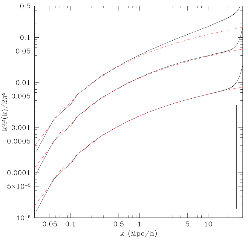
Figure 3 shows the power spectrum of perturbations at redshifts and compares it with the linear theory. A mesh was used to estimate in the simulation, which may underestimate the real spectrum by 3-5 percent at the Nyquist frequency due to the finite smoothing of the density field produced by the Cloud-In-Cell density assignment. Results indicate that the code was evolving the system as it was expected to: linear growth of small perturbations at early stages and at large scales with no suppression at high frequencies.
The number of refinement levels, and thus the force resolution, change with time. For example, there were 8 levels at , and 9 at , which gives the proper resolution of 0.4 kpc. At the tenth level was open with the proper resolution of 0.5 kpc. However, when a level of refinement opens, it contains only a small fraction of volume and particles. Only somewhat later does the number of particles on that level become substantial. This is why the evolution of the force resolution is consistent with nearly constant proper force resolution of 1 kpc from to .
The ART code uses the expansion parameter as the time variable. Each particle moves with its own time-step which depends on the refinement level. The zero-level defines the maximum value of the stepping of the expansion parameter. For Bolshoi for and for later moments. The time-step decreases by a factor of two from one level of refinement to the next. There were ten levels of refinement at the later stages of evolution (). This gives the effective number of 400,000 time-steps.
The initial conditions for the simulation were created using the Zeldovich approximation with particles placed in a homogeneous grid (Klypin & Shandarin, 1983; Klypin & Holtzman, 1997). Bolshoi starts at when the rms density fluctuation in the computational box with particles was equal to . (The Nyquist frequency defines the upper cutoff of the spectrum, with the low cutoff being the fundamental mode.) The initialization code uses the Zeldovich approximation, which provides accurate results only if the density perturbation is less than unity. This should be valid at every point in the volume. In practice, the fluctuations must be even smaller than unity for high accuracy. With independent realizations of the density, one expects to find one particle in the box to have a 6.5 fluctuation. For this particle the density perturbation is ; still below 1.0. The most dense 100 particles are expected to have a density contrast , low enough for the Zeldovich approximation still to be accurate.
The Bolshoi simulation was run at the NASA Ames Research Center on the Pleiades supercomputer. It used 13,824 cores (1728 MPI tasks each having 8 OpenMP threads) and a cumulative 13 Tb of RAM. We saved 180 snapshots for subsequent analysis. The total number of files saved in different formats is about 600,000, which use 100 Tb of disk space.
For some comparisons we also use a catalog of halos for the Via Lactea-II simulation (Diemand et al., 2008). This simulation was run for one isolated halo with maximum circular velocity km s-1. Using approximations for the dark matter profile provided by Diemand et al. (2008), we estimate the virial mass and radius of the halo to be and . Here we use the top-hat model with cosmological constant to estimate the virial radius, as explained in the next section. The Via Lactea-II simulation uses slightly different cosmological parameters as compared with Bolshoi (see Table 1). In particular, the amplitude of perturbations is 10 percent lower: .
3 Halo identification
Let us start with some definitions. A distinct halo is a halo that does not “belong” to another halo: its center is not inside of a sphere with a radius equal to the virial radius of a larger halo. A subhalo is a halo whose center is inside the virial radius of a larger distinct halo. Note that distinct halos may overlap: the same particle may belong to (be inside the virial radius of) more than one halo. We call a halo isolated if there is no larger halo within twice its virial radius. In some cases we study very isolated halos with no larger halo within three times its virial radius.
We use the Bound-Density-Maxima (BDM) algorithm to identify halos in Bolshoi (Klypin & Holtzman, 1997). Appendix A gives some of the details of the halofinder. Knebe et al. (2011) present detailed comparison of BDM with other halofinders and show results of different tests. The code locates maxima of density in the distribution of particles, removes unbound particles, and provides several statistics for halos including virial mass and radius, and maximum circular velocity
| (1) |
Throughout this paper we will use and the term circular velocity to mean maximum circular velocity over all radii . When a halo evolves over time, its may also evolve. This is especially important for subhalos, which can be significantly tidally stripped and can reduce their over time. Thus, we distinguish instantaneous and the peak circular velocity over halo’s history.
We use the virial mass definition that follows from the top-hat model in an expanding Universe with a cosmological constant. We define the virial radius of halos as the radius within which the mean density is the virial overdensity times the mean universal matter density at that redshift. Thus, the virial mass is given by
| (2) |
For our set of cosmological parameters, at the virial radius is defined as the radius of a sphere with overdensity of 360 of the average matter density. The overdensity limit changes with redshift and asymptotically goes to 178 for high . Different definitions are also found in the literature. For example, the often used overdensity 200 relative to the critical density gives mass , which for Milky-Way-mass halos is about 1.2-1.3 times smaller than . The exact relation depends on halo concentration.
Overall, there are about 10 million halos in Bolshoi. Halo catalogs are complete for halos with km s-1 (). We track evolution of each halo in time using 180 stored snapshots. The time difference between consecutive snapshots is rather small: (40-80) Myrs.
4 Halo mass and concentration functions


Throughout most of the paper we characterize halos using their circular velocity. However, tightly correlates with halo mass, as demonstrated in Figure 4. For distinct halos with 90% of halos have their circular velocities within 8% of the median value. Even 99% of halos are within only 15-20%. The variations are substantially larger for subhalos: 90% of subhalos with masses lie within 20% of the median . On average, the circular velocity increases with mass. The relation depends on halo concentration , and, thus, studying this relation gives us a way to estimate without making fits to individual halo profiles. Any halo mass profile can be parameterized as , where and are parameters with mass and radius units and the function is dimensionless. If is the dimensionless radius corresponding to the maximum circular velocity, then we can write the following relation between the maximum circular velocity and the virial mass (Klypin et al., 2001):
| (3) | |||||
| (4) | |||||
| (5) | |||||
| (6) |
Here is the overdensity limit that defines the virial radius; and are the critical density and the contribution of matter to the average density of the Universe. The first two equations are general relations for any density profile. Eqs. (5) and (6) are specific for NFW: is the characteristic radius of the NFW profile, which is the radius at which the logarithmic slope of the density is . At , for our cosmological model, and . Calculating the numerical factors in eqs.(3-6) we get the following relation between virial mass, circular velocity and concentration at :
| (7) |
where mass is in units of , circular velocity is in units of km s-1. This relation gives us an opportunity to estimate halo concentration directly for given virial mass and circular velocity.
Alternatively, one may skip the term and simply use power-law approximations for the relation which give a good fit to numerical data.
For distinct halos:
| (8) |
and for subhalos:
| (9) |
Here velocities are in km s-1 and masses are in units of .
Equations (3 - 6) can be considered as equations for halo concentration: for given , , and one can solve them to find . For quiet halos the result must be the same as what one gets from fitting halo density profiles with the NFW approximation: two independent parameters (in our case and ) uniquely define the density profile. However, by using only two parameters, we are prone to fluctuations. In order to reduce the effects of fluctuations we apply eqs. (3 - 6) to the median values of for each mass bin. For each mass bin with the average we find the median circular velocity . We then solve equations (3-6) and get median halo concentrations . One can also find concentration for each halo and then take the median - result is the same because for a given mass the relation between and is monotonic. This procedure minimizes effects of fluctuations and gives the median halo concentration for a given mass. Muñoz-Cuartas et al. (2010) applied our method to their simulations and reproduced results of direct density profile fitting. Prada et al. (2011) state that this method recovers results of halo concentrations in MS-I (Neto et al., 2007) with deviations of less than 5 percent over the whole range of masses in the simulation.
Figure 5 shows the concentrations for redshifts . For redshift zero we get the following approximation:
| (10) |
for distinct halos. For subhalos we find:
| (11) |
Subhalos are clearly more concentrated than distinct halos with the same mass, which is likely caused by tidal stripping. The differences between subhalos and distinct halos on average are not large: a 30% effect in halo concentration.
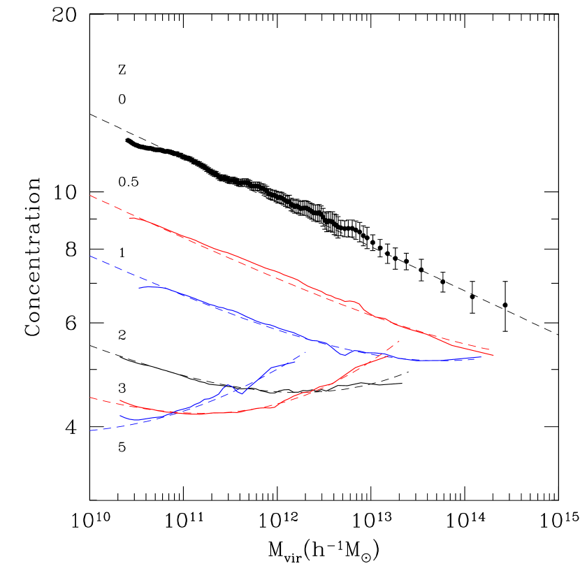
We also study the evolution of distinct halo concentration with redshift. Figure 5 shows the concentrations for redshifts . Results can be approximated using the following functions:
| (12) | |||||
where and are two free factors for each . Table 3 gives the parameters for this approximation at different redshifts. For convenience we also give the concentration for a virial mass and the minimum value of concentration . The simulation box for the Bolshoi is not large enough to find whether there is a minimum concentration for . For these epochs the Table gives the value of concentration at as predicted by the analytical fits.

The curves in Figure 5 look different for different redshifts. Typically the concentration declines with redshift and the shape of the curves evolves. Another interesting result is that the high- curves show that the halo concentration has an upturn: for the most massive halos the concentration increases with mass. In order to demonstrate this more clearly, we study in more detail the evolution with redshift of the halo concentration for halos with two masses: and . Note that the masses are the same at different redshifts. So, this is not the evolution of the same halos. Figure 6 shows the results. Just as expected, in both cases at low redshifts the halo concentration declines with redshift. The decline is not as steep as often assumed ; it is significantly shallower even at low . For a power-law approximation is a much better fit, where is the linear growth factor. It is also a better approximation because the evolution of concentration should be related with the growth of perturbations, not with the expansion of the universe. At larger the concentration flattens and slightly increases at . The upturn is barely visible for the larger mass, but it is clearly seen for the mass halos. These and other results show that the concentration in the upturn does not increase above though it may be related with the finite box size of our simulation. There is also an indication that there is an absolute minimum of the concentration at high redshifts. Relaxed halos333 Relaxed halos are defined as halos with offset parameter and with spin parameter , where is the distance from the halo center to its center of mass in units of the virial radius. show a slightly stronger upturn indicating that non-equilibrium effects are not the prime explanation for the increasing of the halo concentration.
The following analytical approximations provide fits for the evolution of concentrations for fixed masses as shown in Figure 6:
| (13) |
here is the linear growth factor of fluctuations normalized to be and is a free parameter, which for the masses presented in the Figure is for and for ten times more massive halos with .
| Redshift | ||||
|---|---|---|---|---|
| 0.0 | 9.60 | – | – | 9.60 |
| 0.5 | 7.08 | 5.2 | 7.2 | |
| 1.0 | 5.45 | 5.1 | 5.8 | |
| 2.0 | 3.67 | 4.6 | 4.6 | |
| 3.0 | 2.83 | 4.2 | 4.4 | |
| 5.0 | 2.34 | 4.0 | 5.0 |

It is interesting to compare these results with other simulations. Zhao et al. (2003, 2009) were the first to find that the concentration flattens at large masses and at high redshifts. Their estimates of the minimum concentration are compatible with our results. Figure 2 in Zhao et al. (2003) shows an upturn in concentration at . However, the results were noisy and inconclusive: the text does not even mention it.
Macciò et al. (2008) present results that can be directly compared with ours because they use the same definition of the virial radius and estimate masses within spherical regions. Their models named WMAP5 have parameters that are very close to those of Bolshoi. There is one potential issue with their simulations. Macciò et al. (2008) use a set of simulations with each simulation having a small number of particles and either a low resolution, if the box size is large, or very small box, if the resolution is small. For all the halos in their simulations the approximation for concentration is . Bolshoi definitely gives more concentrated halos. The largest difference is for cluster-size halos. For our results give while Macciò et al. (2008) predict – a 40% difference. The difference gets smaller for galaxy-size halos: 14% for and 2% for . Comparing results for relaxed halos we find that the disagreement is smaller. Muñoz-Cuartas et al. (2010) give for as compared with our results (also for relaxed halos) of - a 3% difference. For clusters with the disagreement is 18%.

We can also compare our results with those of MS-I (Neto et al., 2007) though MS-I has different cosmological parameters and a different power spectrum. Because the analysis of MS-I was done for the overdensity 200, we also made halo catalogs for this definition of halos. Neto et al. (2007) give the following approximation for all halos: . For halos in the Bolshoi simulation . Thus the MS-I is 8% larger than the concentrations in Bolshoi for , with a small (10%) difference for . For in the MS-II and Aquarius simulations Boylan-Kolchin et al. (2009) give an even larger concentration of , which is 1.3 times larger than what we get from Bolshoi. Most of the differences are likely due to the larger amplitude of cosmological fluctuations in MS simulations because of the combination of a larger and a steeper spectrum of fluctuations.
The mass function of distinct halos is a classical cosmological result (e.g., Warren et al., 2006; Reed et al., 2007; Tinker et al., 2008; Macciò et al., 2008; Reed et al., 2009). Figure 7 presents the results for the Bolshoi simulation together with the predictions of the Sheth-Tormen approximation (Sheth & Tormen, 2002, ST, see also Appendix B). We find that the ST approximation gives an accurate fit for with the deviations less than 10 percent for masses ranging from to . However, the ST approximation overpredicts the abundance of halos at higher redshifts. For example, at for halos with the ST approximation gives a factor of 1.5 more halos as compared with the simulation. At redshift ten the ST approximation gives a factor of ten more halos than what we find in the simulation.
We introduce a simple correction factor which brings the analytical predictions much closer to the results of simulations. We find that the ST approximation multiplied by the following factor gives less than 10 percent deviations for masses and redshifts :
| (14) |
where is the linear growth rate factor normalized to unity at (see eq. (B2)).
Our results are in good agreement with Tinker et al. (2008), who present the evolution of the mass function for for halos defined using the spherical overdensity method. At redshift zero, their mass function for overdensity relative to the mean mass density is 20% above the ST approximation. This is expected because masses defined with spherical overdensity are typically 10-20% larger than virial masses, which are used in our paper. Results in Tinker et al. (2008) together with our work indicate that at higher redshifts the mass function gets more and more below the ST approximation. In addition, the shape of the mass function in simulations gets steeper: there is a larger disagreement at larger masses. Tinker et al. (2008) argue that this behavior indicates that the mass function is not “universal”: it does not scale with the redshift only as a function of the amplitude of perturbations on scale (see Appendix B for definitions). Our results extend this trend to redshifts at least as large as . Our results also qualitatively agree with Cohn & White (2008), who present spherical overdensity halo masses at . They also find substantially lower mass functions as compared with the ST approximation, though the differences with the approximation are somewhat smaller than what we find.

These results are at odds with those obtained with the Friends-Of-Friends (FOF) method (e.g. Lukić et al., 2007; Reed et al., 2007, 2009; Cohn & White, 2008). The FOF halo mass function scales very close to the “universal” behavior. The reason for the disagreement between spherical overdensity and FOF halo finding methods is likely related with the fact that FOF has a tendency to link together structures before they become a part of a virialized halo. This happens more often with the rare most massive halos, which have a tendency to be out of equilibrium and in the process of merging. As a result of this, FOF masses are artificially inflated. Cohn & White (2008) studied case-by-case some halos at and conclude that in their simulations FOF assigned to halos almost twice more mass. Comparison of the ST predictions with the Bolshoi results shown in Figure 7 points to the difference of a factor of 2.5 in mass for . Because of the steep decline of the mass function, a factor of 2.5 increase in mass translates to a factor of ten increase in the number-density of halos. This correction to the FOF masses must be taken into account when making any estimates of the frequency of appearance of high- objects.
In Appendix C we also directly compare FOF masses with those obtained with the BDM code. At the FOF masses with the linking parameter were on average 1.4 times larger than the BDM masses. In addition, the spread of estimates was very large with FOF in many cases giving 3-5 times larger masses than BDM. Analysis of individual cases shows that this happens because FOF links large fragments of filaments, not just an occasional neighboring halo. The situation is different at . Here both BDM and FOF () give remarkably similar results, though some spread is still present (Tinker et al., 2008). We speculate that the difference in the behavior at high and low is related with the slope of the power spectrum of perturbations probed by halos at different redshifts.
These differences between different definitions of masses and radii of halos indicate the inherent weakness of masses as halo properties: in the absence of a well defined physical process responsible for halo formation, masses are defined somewhat arbitrarily. We know that halos do not form according to the often used top-hat model. We also know that the virial radius is ill-defined for non-isolated interacting objects. Nevertheless, we use one definition or another and we pay a price for this vagueness. These uncertainties in masses also motivate us to use another, – much better defined quantity – the maximum circular velocity.
5 Halo velocity function
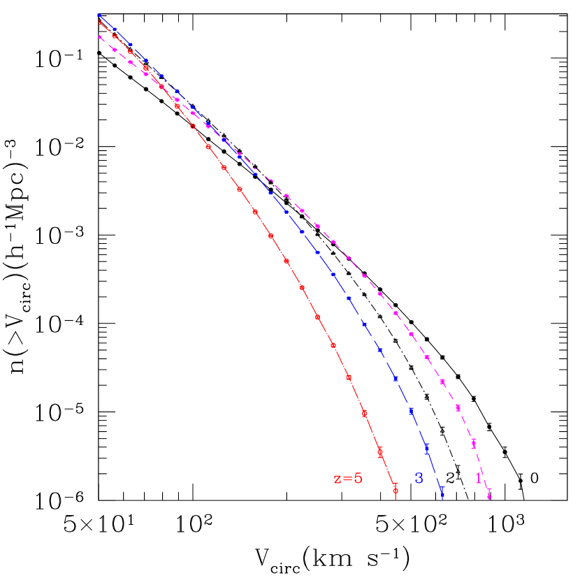
The velocity function for distinct halos is shown in Figure 8. It declines very steeply with velocity. At small velocities the power slope is –3 with an exponential cutoff at large velocities. We find that at all redshifts the cumulative velocity function can be accurately approximated by the following expression:
| (15) |
where the parameters , , and are functions of redshift. For we find
| (16) | |||||
The evolution of the parameters should not directly depend on the redshift, but on the amplitude of perturbations. Indeed, when we plot the parameters as functions of as predicted by the linear theory at different redshifts, the functions are very close to power-laws as demonstrated by Figure 9. We find the following fits to the parameters:
| (17) | |||||
6 Abundance of Subhalos

Figure 10 shows the cumulative velocity function of all subhalos in Bolshoi regardless of the circular velocity of their host halos. We use maximum circular velocities over the whole evolution for both subhalos and distinct halos. The top panel shows the ratio of the number of subhalos to the number of distinct halos with the same limit on the circular velocity. Note that for given most of the halos are distinct. This may sound a bit counter intuitive. Because each distinct halo has many subhalos, one would naively expect that there are many more satellites as compared with distinct halos. This is not true. The number of satellites is large, but most are small. When we count small distinct halos, their number increases very fast and we always end up with more distinct halos at a given circular velocity. The abundance of subhalos can be approximated with the same function given by eq. (15) as for the distinct halos. However, the parameters of the approximation are different. For subhalos that exist at and for which we use peak velocities over their history of evolution, we find:
| (18) |
The remarkable similarity of the shapes of the velocity functions of halos and subhalos suggests a simple interpretation for the difference in their parameters: subhalos were typically accreted at the epoch when the velocity function of distinct halos had the same parameters and as the velocity function of subhalos at present. For the parameters given by eqs. (17,18) we get a typical accretion redshift .
In order to study statistics of subhalos belonging to different parent halos we split our sample of distinct halos into subsamples with different ranges of circular velocities. For each subhalo we use either its circular velocity or the peak value over its entire evolution. Figure 11 shows both the present day and the peak velocity distribution functions for distinct halos with masses and velocities ranging from galaxy-size halos to clusters of galaxies. The average circular velocities for each bin presented in the figure are (from bottom to top): km s-1. The number of halos in each bin varies from 200 for the most massive halos () to 30000 for the least massive halos with . The increase in the abundance of substructure for more massive hosts is consistent with the results of Gao et al. (2004), who give a factor of 2.0-2.5 increase for host halos from mass to . van den Bosch et al. (2005); Taylor & Babul (2005); Zentner et al. (2005) came to similar conclusions using their (semi)analytic models.
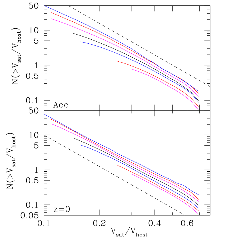
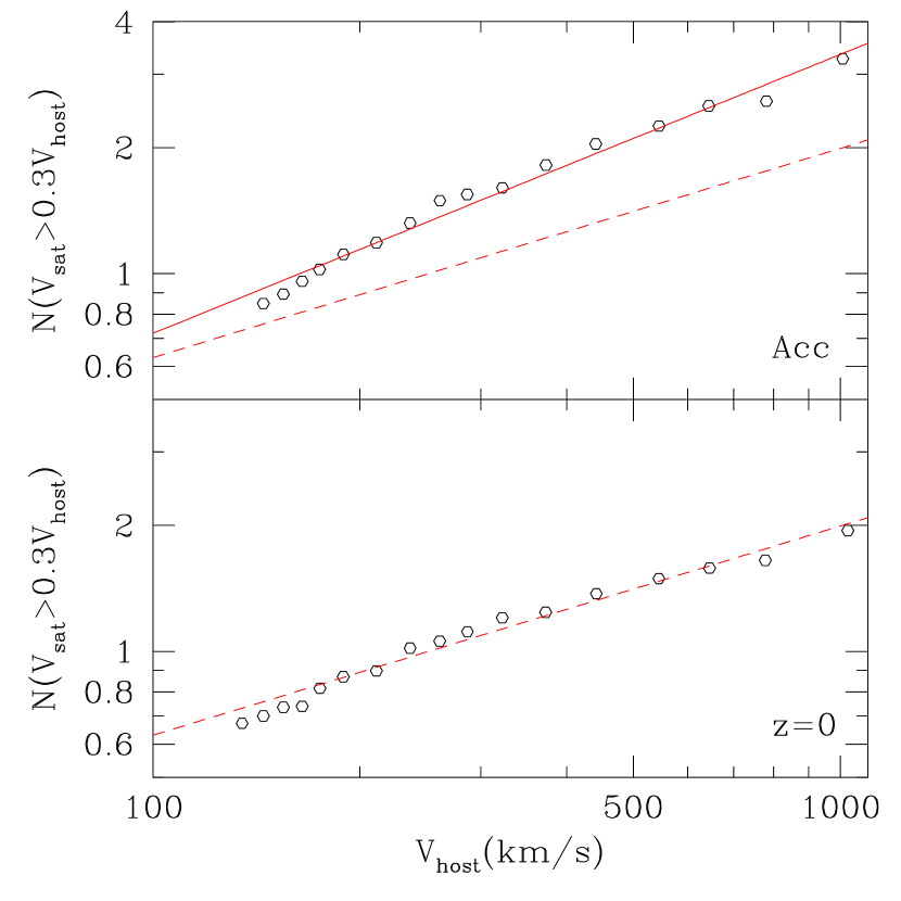
In order to more accurately measure the dependence of the abundance of subhalos on the circular velocity of the host halo, we analyze the number of satellites with circular velocities larger than 0.3 of the circular velocity of their hosts: . This approximately corresponds to the mass ratio of . The threshold of 0.3 is a compromise between the statistics of satellites and the numerical resolution of the simulation. Figure 12 shows the number of satellites for hosts ranging from 150 km s-1 to 1000 km s-1. The number of satellites scales as a power-law with the slope depending on how the circular velocity is estimated. For the velocities the slope is , and it is larger for the peak velocities: .
There is an indication that the dependence of the cumulative number of satellites on their circular velocity gets slightly shallower for more massive host halos. Figure 13 illustrates the point. Here we study the most massive (but also rare) halos. Again, the number of satellites is approximated by a power-law. However, the slope is about , which is somewhat shallower than the slope found for smaller host halos.
We compare some of our results with the Via Lactea-II (VL-II) simulation (Diemand et al., 2008). We do not use the published results because the analysis of VL-II was done using overdensity 180 relative to the matter density, which gives a larger radius for halos as compared with the virial radius. We use the halo catalog of VL-II, which lists coordinates and circular velocities of individual halos. We also use published parameterization of the dark matter density in order to estimate the virial radius of VL-II. When comparing with VL-II, we select halos in Bolshoi in a narrow range of circular velocities km s-1. There are 4960 of those with the average virial mass of , which is close to the virial mass of Via Lactea II. Figure 14 presents results of the velocity function of subhalos in those host halos. The dashed line in the figure is the power law , which gives a good fit to the data for a wide range of circular velocities from 4 km s-1 to 100 km s-1. Bolshoi has slightly more subhalos by about 10%. This is a small difference and it goes in line with expectation that a smaller normalization of cosmological fluctuations gives fewer subhalos. In the same vein, the Aquarius simulations have an even higher (by 30% as compared to VL-II) number of subhalos, probably because of an even larger amplitude.
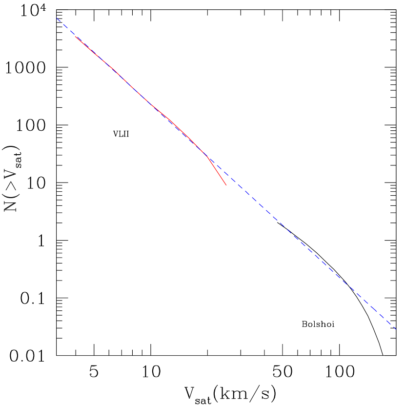
Summarizing all the results, we conclude that the cumulative velocity function of subhalos can be reasonably accurately approximated by the power law:
| (19) | |||||
| (20) |
where the circular velocity of the host is given in units of km s-1. Again, these results are broadly consistent with the -body simulations of Gao et al. (2004) and with the semianalytic models of van den Bosch et al. (2005); Taylor & Babul (2005) and Zentner et al. (2005). For peak circular velocities we obtain:
| (21) |
7 The spatial distribution of satellites

The spatial distribution of satellites has numerous astrophysical applications. Among others, these include the survivability of dark matter subhalos (e.g., Moore et al., 1996; Klypin et al., 1999; Colín et al., 1999), the potential annihilation signal of dark matter (e.g., Kuhlen et al., 2008; Springel et al., 2008; Ando, 2009), and motion of satellites as a probe for masses of isolated galaxies and groups (e.g., Prada et al., 2003; Klypin & Prada, 2009; More et al., 2009). The relative abundance of satellites and dark matter is a form of bias. Thus, studying the distribution of satellites in simulations sheds light on the physics of bias and, thus, on the formation of dwarf galaxies. There is an additional reason to study the satellites in the Bolshoi simulation: comparison with high resolution simulations such as Via Lactea gives an additional test on resolution effects and provides limits of the applicability of the simulation.
The spatial distribution of satellites has been extensively studied in simulations (Ghigna et al., 1998, 2000; Nagai & Kravtsov, 2005; Diemand et al., 2008; Springel et al., 2008; Angulo et al., 2009). One of the main issues regarding satellites is to what degree their distribution is more extended than that of the dark matter. As a small halo falls into the gravitational potential of a larger halo, it experiences tidal stripping and dynamical friction. It may also experience interaction with other subhalos before and during infall. Tidal stripping reduces the mass of subhalos, resulting in a very strong radial bias: subhalos selected by mass have relatively low number-density in the central region of their hosts. However, stripping affects much less the central parts of subhalos. This is why the distribution of subhalos is more concentrated when selected by their circular velocity (Nagai & Kravtsov, 2005). Depending on the mass and concentration of the subhalo and on its trajectory, the role of different physical effects may vary. Interplay of these processes results in a complicated picture of the distribution of the satellites. Numerical effects add to the complexity of the situation: it is a challenge to preserve and to identify small subhalos through the whole history of evolution of the Universe.
The traditional way of displaying results is to normalize both the dark matter and satellites to the average mass inside the virial radius. When presented in this way, results routinely show that there are relatively more satellites in the outer parts of halos. For example, Angulo et al. (2009) find that independently of subhalo mass, subhalos are a factor of two more abundant than dark matter around the virial radius of their hosts. If that were correct, this would imply some kind of physical mechanism to produce more satellites outside of the virial radius, a far-reaching conclusion. However, below we show that this not correct.
The main issue here is the normalization. If a simulation includes only a small region, a typical setup for modern high-resolution simulations, there is no sensible way to normalize satellites. This is not the case given the statistics of Bolshoi. We can reliably normalize the abundance of even halos with small mass and circular velocities. The velocity function of all distinct halos is given by eq. (15). There are 20-25% subhalos at given circular velocity. Using the velocity function and the fraction of subhalos from Bolshoi, we estimate the average number of all halos with any given . These estimates are used to normalize the number-density profile of subhalos in VL II presented in Figure 15. A comparison with the dark matter profile is quite interesting: there is very little bias in the Via Lactea distribution of subhalos for radii . Subhalos are not more extended as compared with the dark matter. However, Via Lactea-II is just one halo and there may be some effects related with cosmic variance. We use halos in Bolshoi that have similar characteristics as Via Lactea-II: very isolated halos (no equal mass halo inside ) and circular velocities in the range km s-1 with corresponding masses . For Bolshoi halos we find a small 10% antibias. In the inner regions () the number density of satellites goes below the results of Via Lactea, but the difference is not large: 20-30%. Some of the differences with Via Lactea-II may be real because subhalos in Bolshoi are more massive, and, thus, they must experience stronger dynamical friction. However, it is more likely that most of the differences are numerical: after all, Bolshoi has substantially worse resolution than Via Lactea-II. Regardless of the cause of those small differences, it is quite remarkable that simulations with five orders of magnitude difference in mass resolution produce results that deviate only by 10-20%.
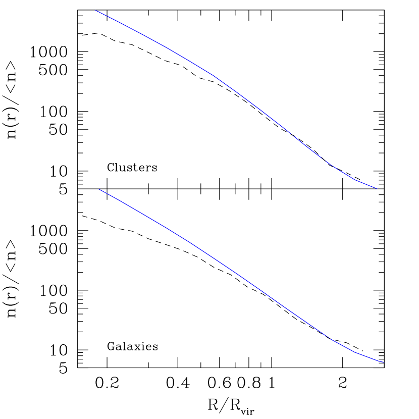
Comparison with Via Lactea-II is difficult because for these masses () Bolshoi has only a few subhalos per each host. In order to have a better picture of the spatial distribution of satellites, we study more massive halos for which our resolution is relatively better. Again, we select isolated halos: those with no larger halo within twice the virial radius. Figure 16 shows the results for hosts with very different masses. The top panel shows results for 82 halos with circular velocities in the range 900-1100 km s-1 (average virial mass ). The bottom panel shows 2200 halos with km s-1 and average . Results are very similar for such different host halos: satellites follow the dark matter very closely for radii with possible small (10%) antibias. In the central region the subhalo abundance goes below the dark matter by a factor of 2-2.5 at .
It is interesting to compare the Bolshoi results with Nagai & Kravtsov (2005), who present profiles for 8 clusters with almost the same masses as in the top panel of our Figure 16. If we change their normalization for subhalos selected by present-day circular velocity (their Figure 3) in such a way that the dark matter profile matches the overdensity of satellites at the virial radius (we use a factor of 0.8 to match our definition of virial radius), then there is excellent agreement with Bolshoi, with both simulations giving the ratio of the dark matter density to the number-density of satellites at .
8 Conclusions
Using the large halo statistics and high resolution of the Bolshoi simulation we study numerous properties of halos and subhalos. We present accurate analytical approximations for such characteristics as the halo and subhalo abundances and concentrations, the velocity functions, and the number-density profiles of subhalos. Detailed discussions of different statistics have already been given in relevant sections of the text. Here we present a short summary of our main conclusions.
Velocity function. Our main property of halos is their maximum circular velocity . As compared with virial masses, circular velocities are better quantities to characterize the physical parameters of the central regions of dark matter halos. As such, they are better quantities to relate the dark matter halos and galaxies, which they host. We present the halo velocity functions at different redshifts and show that they can be accurately described by eqs. (15-17). The halo circular velocity function declines as a power-law at small velocities and has a quasi-exponential cutoff at large circular velocities.
Mass function of distinct halos. We find that the ST approximation (Sheth & Tormen, 2002) gives an accurate fit to the redshift-zero mass function: errors are less than 10% for masses in the range . However, the approximation overpredicts the halo abundance at higher redshifts and gives a factor of ten more halos than the Bolshoi simulation at . The correction factor eq. (14) brings the accuracy of the approximation back to the % level for redshifts . It also breaks the universality of the fit: the mass function cannot be written as a function of only the rms fluctuation on mass scales . These results depend on how halos are defined with the Friends-Of-Friends algorithm giving different answers than the spherical overdensity method. See Appendix C for details.
Concentrations of halos. The halo concentration appears to be more complex than previously envisioned. For a given redshift , the concentration first declines with increasing mass. Then it flattens-out and reaches a minimum of with the value of the minimum changing with redshift. At even larger masses starts to slightly increase. This “up-turn” in the concentration is a weak feature: the change in concentration is only 20%. Moreover, it cannot be detected at low redshifts, . If our estimates are correct, at the upturn should start at masses about - clusters this massive do not exist. However, at the upturn is visible at the very massive tail of the mass function. It is not clear what causes the upturn. The upturn is even stronger for relaxed halos, which indicates that non-equilibrium effects cannot be the reason for the upturn. At large redshifts the halos that show the upturn are very rare: their mass is much larger than the characteristic mass of halos existing at that time. Most of them likely experience a very fast growth. They also represent very high- peaks of the density field. It is known that the statistics of rare peaks are different from those of more “normal” peaks (Bardeen et al., 1986). One may speculate that this may result in a change in halo concentration. More extensive analysis of halo concentrations is given in Prada et al. (2011).
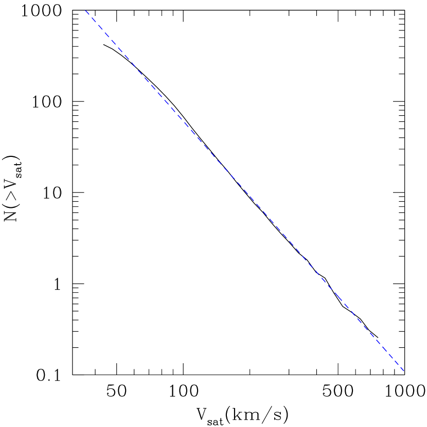
Subhalo abundance. The cumulative abundance of satellites is a power-law with a steep slope: . Combing our results with those of the Via Lactea-II simulation (Diemand et al., 2008), we show that the power-law extends at least from 4 km s-1 to 150 km s-1for Milky-Way-mass halos and yields the correct abundance of large satellites such as the Large Magellanic Cloud (Busha et al., 2010). The abundance of satellites increases with the circular velocity and mass of the host halo as . For example, this means that in relative units a cluster of galaxies has 2.5 times more satellites than the Milky Milky Way, in good agreement with previous numerical results (Gao et al., 2004). Eqs. (20-21) give approximations for the abundance of satellites.
Subhalo number-density distribution. One of the main issues here is the number-density of satellites relative to the dark matter in the outer regions of halos. Some previous simulations indicated substantial (a factor of two) overabundance of satellites around the virial radius. We do not confirm this conclusion. Our re-analysis of the Via Lactea-II simulation as well as the results from the Bolshoi simulation unambiguously show that there is no overabundance of satellites. In the Via Lactea-II simulation the satellites follow very closely the distribution of dark matter for radii . In the Bolshoi simulation we find a small (10%) antibias at the virial radius.
References
- Allgood et al. (2006) Allgood, B., Flores, R. A., Primack, J. R., Kravtsov, A. V., Wechsler, R. H., Faltenbacher, A., & Bullock, J. S. 2006, MNRAS, 367, 1781
- Ando (2009) Ando, S. 2009, Phys. Rev. D, 80, 023520
- Angulo et al. (2009) Angulo, R. E., Lacey, C. G., Baugh, C. M., & Frenk, C. S. 2009, MNRAS, 399, 983
- Angulo & White (2009) Angulo, R. E., & White, S. D. M. 2009, arXiv:0912.4277
- Bardeen et al. (1986) Bardeen, J. M., Bond, J. R., Kaiser, N., & Szalay, A. S. 1986, ApJ, 304, 15
- Blumenthal et al. (1984) Blumenthal, G. R., Faber, S. M., Primack, J. R., & Rees, M. J. 1984, Nature, 311, 517
- Boylan-Kolchin et al. (2009) Boylan-Kolchin, M., Springel, V., White, S. D. M., & Jenkins, A. 2009, arXiv:0911.4484
- Boylan-Kolchin et al. (2009) Boylan-Kolchin, M., Springel, V., White, S. D. M., Jenkins, A., & Lemson, G. 2009, MNRAS, 398, 1150 (MS-II)
- Bryan & Norman (1998) Bryan, G. L., & Norman, M. L. 1998, ApJ, 495, 80
- Bullock et al. (2001) Bullock, J. S., Dekel, A., Kolatt, T. S., Kravtsov, A. V., Klypin, A. A., Porciani, C., & Primack, J. R. 2001, ApJ, 555, 240
- Busha et al. (2010) Busha, M. T., Wechsler, R. H., Behroozi, P. S., Gerke, B. F., Klypin, A. A., & Primack, J. R. 2010, arXiv:1011.6373
- Carroll et al. (1992) Carroll, S. M., Press, W. H., & Turner, E. L. 1992, ARA&A, 30, 499
- Cohn & White (2008) Cohn, J. D., & White, M. 2008, MNRAS, 385, 2025
- Colín et al. (1999) Colín, P., Klypin, A. A., Kravtsov, A. V., & Khokhlov, A. M. 1999, ApJ, 523, 32
- Davis et al. (1985) Davis, M., Efstathiou, G., Frenk, C. S., & White, S. D. M. 1985, ApJ, 292, 371
- Diemand et al. (2008) Diemand, J., Kuhlen, M., Madau, P., Zemp, M., Moore, B., Potter, D., & Stadel, J. 2008, Nature, 454, 735 (VL-II)
- Dunkley et al. (2009) Dunkley, J., et al. 2009, ApJS, 180, 306
- Gao et al. (2004) Gao, L., White, S. D. M., Jenkins, A., Stoehr, F., & Springel, V. 2004, MNRAS, 355, 819
- Ghigna et al. (1998) Ghigna, S., Moore, B., Governato, F., Lake, G., Quinn, T., & Stadel, J. 1998, MNRAS, 300, 146
- Ghigna et al. (2000) Ghigna, S., Moore, B., Governato, F., Lake, G., Quinn, T., & Stadel, J. 2000, ApJ, 544, 616
- Gnedin et al. (2007) Gnedin, O. Y., Weinberg, D. H., Pizagno, J., Prada, F., & Rix, H.-W. 2007, ApJ, 671, 1115
- Gottloeber & Klypin (2008) Gottloeber, S., & Klypin, A. 2008, in ”High Performance Computing in Science and Engineering Garching/Munich 2007”, Eds. S. Wagner et al, Springer, Berlin 2008 (arXiv:0803.4343)
- Henry et al. (2009) Henry, J. P., Evrard, A. E., Hoekstra, H., Babul, A., & Mahdavi, A. 2009, ApJ, 691, 1307
- Hinshaw et al. (2009) Hinshaw, G., et al. 2009, ApJS, 180, 225
- Jarosik et al. (2010) Jarosik, N., et al. 2010, arXiv:1001.4744
- Jenkins et al. (1998) Jenkins, A., et al. 1998, ApJ, 499, 20
- Klypin & Shandarin (1983) Klypin, A. A., & Shandarin, S. F. 1983, MNRAS, 204, 891
- Klypin et al. (1996) Klypin, A., Primack, J., & Holtzman, J. 1996, ApJ, 466, 13
- Klypin & Holtzman (1997) Klypin, A., & Holtzman, J. 1997, arXiv:astro-ph/9712217
- Klypin et al. (1999) Klypin, A., Gottlöber, S., Kravtsov, A. V., & Khokhlov, A. M. 1999, ApJ, 516, 530
- Klypin et al. (2001) Klypin, A., Kravtsov, A. V., Bullock, J. S., & Primack, J. R. 2001, ApJ, 554, 903
- Klypin & Prada (2009) Klypin, A., & Prada, F. 2009, ApJ, 690, 1488
- Klypin et al. (2009) Klypin, A., Valenzuela, O., Colín, P., & Quinn, T. 2009, MNRAS, 398, 1027
- Knebe et al. (2011) Knebe, A., et al. 2011, MNRAS, 819
- Komatsu et al. (2009) Komatsu, E., et al. 2009, ApJS, 180, 330
- Kravtsov et al. (1997) Kravtsov, A. V., Klypin, A. A., & Khokhlov, A. M. 1997, ApJS, 111, 73
- Kravtsov (1999) Kravtsov, A. V. 1999, Ph.D. Thesis
- Kravtsov et al. (2004) Kravtsov, A. V., Berlind, A. A., Wechsler, R. H., Klypin, A. A., Gottlöber, S., Allgood, B., & Primack, J. R. 2004, ApJ, 609, 35
- Kuhlen et al. (2008) Kuhlen, M., Diemand, J., & Madau, P. 2008, ApJ, 686, 262
- Lahav et al. (1991) Lahav, O., Lilje, P. B., Primack, J. R., & Rees, M. J. 1991, MNRAS, 251, 128
- Lewis et al. (2000) Lewis, A., Challinor, A., & Lasenby, A. 2000, ApJ, 538, 473
- Lukić et al. (2007) Lukić, Z., Heitmann, K., Habib, S., Bashinsky, S., & Ricker, P. M. 2007, ApJ, 671, 1160
- Macciò et al. (2007) Macciò, A. V., Dutton, A. A., van den Bosch, F. C., Moore, B., Potter, D., & Stadel, J. 2007, MNRAS, 378, 55
- Macciò et al. (2008) Macciò, A. V., Dutton, A. A., & van den Bosch, F. C. 2008, MNRAS, 391, 1940
- Mantz et al. (2008) Mantz, A., Allen, S. W., Ebeling, H., & Rapetti, D. 2008, MNRAS, 387, 1179
- Melott et al. (1983) Melott, A. L., Einasto, J., Saar, E., Suisalu, I., Klypin, A. A., & Shandarin, S. F. 1983, Physical Review Letters, 51, 935
- Moore et al. (1996) Moore, B., Katz, N., & Lake, G. 1996, ApJ, 457, 455
- More et al. (2009) More, S., van den Bosch, F. C., Cacciato, M., Mo, H. J., Yang, X., & Li, R. 2009, MNRAS, 392, 801
- Muñoz-Cuartas et al. (2010) Muñoz-Cuartas, J. C., Macciò, A. V., Gottlöber, S., & Dutton, A. A. 2010, MNRAS, 1685
- Nagai & Kravtsov (2005) Nagai, D., & Kravtsov, A. V. 2005, ApJ, 618, 557
- Navarro et al. (1996) Navarro, J. F., Frenk, C. S., & White, S. D. M. 1996, ApJ, 462, 563
- Neto et al. (2007) Neto, A. F., et al. 2007, MNRAS, 381, 1450
- Prada et al. (2003) Prada, F., et al. 2003, ApJ, 598, 260
- Prada et al. (2011) Prada, F., et al. 2011, in preparation.
- Primack & Blumenthal (1984) Primack, J. R., & Blumenthal, G. R. 1984, NATO ASIC Proc. 117: Formation and Evolution of Galaxies and Large Structures in the Universe, 163
- Reed et al. (2007) Reed, D. S., Bower, R., Frenk, C. S., Jenkins, A., & Theuns, T. 2007, MNRAS, 374, 2
- Reed et al. (2009) Reed, D. S., Bower, R., Frenk, C. S., Jenkins, A., & Theuns, T. 2009, MNRAS, 394, 624
- Rozo et al. (2009) Rozo, E., et al. 2009, ApJ, 699, 768
- Seljak & Zaldarriaga (1996) Seljak, U., & Zaldarriaga, M. 1996, ApJ, 469, 437
- Sheth & Tormen (2002) Sheth, R. K., & Tormen, G. 2002, MNRAS, 329, 61
- Spergel et al. (2003) Spergel, D. N., et al. 2003, ApJS, 148, 175
- Springel et al. (2005) Springel, V., et al. 2005, Nature, 435, 629 (MS-I)
- Springel et al. (2008) Springel, V., et al. 2008, MNRAS, 391, 1685
- Springel et al. (2008) Springel, V., et al. 2008, Nature, 456, 73
- Taylor & Babul (2005) Taylor, J. E., & Babul, A. 2005, MNRAS, 364, 515
- Tinker et al. (2008) Tinker, J., Kravtsov, A. V., Klypin, A., Abazajian, K., Warren, M., Yepes, G., Gottlöber, S., & Holz, D. E. 2008, ApJ, 688, 709
- Trujillo-Gomez et al. (2010) Trujillo-Gomez, S., Klypin, A., Primack, J., & Romanowski, A. 2010, arXiv:1005.1289
- van den Bosch et al. (2005) van den Bosch, F. C., Tormen, G., & Giocoli, C. 2005, MNRAS, 359, 1029
- Vikhlinin et al. (2009) Vikhlinin, A., et al. 2009, ApJ, 692, 1060
- Warren et al. (2006) Warren, M. S., Abazajian, K., Holz, D. E., & Teodoro, L. 2006, ApJ, 646, 881
- Wechsler et al. (2002) Wechsler, R. H., Bullock, J. S., Primack, J. R., Kravtsov, A. V., & Dekel, A. 2002, ApJ, 568, 52
- Zentner et al. (2005) Zentner, A. R., Berlind, A. A., Bullock, J. S., Kravtsov, A. V., & Wechsler, R. H. 2005, ApJ, 624, 505
- Zhao et al. (2003) Zhao, D. H., Jing, Y. P., Mo, H. J., & Börner, G. 2003, ApJ, 597, L9
- Zhao et al. (2009) Zhao, D., Jing, Y. P., Mo, H. J., & Börner, G., 2009, ApJ, 707, 354
Appendix A APPENDIX: Bound Density Maxima halofinder
We use a parallel (MPI+OpenMP) version of the Bound-Density-Maxima algorithm to identify halos in Bolshoi (Klypin & Holtzman, 1997). For detailed comparison with other halofinders see Knebe et al. (2011). The code detects both distinct halos and subhalos. The code locates maxima of density in the distribution of particles, removes unbound particles, and provides several statistics for halos including virial mass and radius, as well as maximum circular velocity. The parameters of the BDM halo finder were set such that the density maxima are not allowed to be closer than . We keep only the more massive density maximum 444We keep the peak that has the largest mass inside a sphere of radius if that happens. This is mostly done to save computer time. It is also consistent with the force resolution of Bolshoi. Halo catalogs obtained with a smaller minimum separation of did not include more halos.
Removal of unbound particles is done iteratively. It goes in steps:
-
1.
Find the bulk velocity of a halo: the velocity with which the halo moves in space. The rms velocities of individual particles are later found relative to this velocity. We use the central region of the halo (the 30 particles closest to the halo center) to find the bulk velocity.
-
2.
Find the halo radius: the minimum of the virial radius and the radius of the declining part of the density profile (radius of the density minimum, if it exists).
-
3.
Find the rms velocity of dark matter particles and the circular velocity profile. Estimate the halo concentration.
-
4.
Find the escape velocity as a function of radius and remove particles that exceed the escape velocity. Use only bound particles for the next iteration.
The whole procedure (steps 1–4) is repeated 4 times. If the mass or radius of a halo are too small (too few particles), the density maximum is removed from the list of halo candidates.
If two halos (a) are separated by less than one virial radius, (b) have masses that differ by less than a factor of 1.5, and (c) have a relative velocity less than 0.15 of the rms velocity of dark matter particles inside the halos, we remove the smaller halo and keep only the larger one. This is done to remove a defect of halo-finding where the same halo is identified more than once. This removal of “duplicates” (halos with nearly the same mass, position, and velocity) happens only during major merger events when instead of two merging nearly equal-mass halos the halo finder sometimes finds 3-5 halos. Unfortunately, this also has the side effect of removing one of the major merger halos. This is a relatively rare event and it affects only the very tip of the subhalo velocity function.
We use the virial mass definition that follows from the top-hat model in an expanding Universe with a cosmological constant. We define the virial radius of halos as the radius within which the mean density is the virial overdensity times the mean universal matter density at that redshift. Thus, the virial mass is given by
| (A1) |
Eq. (B1) gives an analytical approximation for . For our set of cosmological parameters, at the virial radius is defined as the radius of a sphere with overdensity of 360 times the average matter density. The overdensity limit changes with redshift and asymptotically approaches 178 for high .
Overall, there are about 10 million halos in Bolshoi (8.8 M at , 12.3 M at , 4.8 M at ). Halo catalogs are complete for halos with km s-1 (). We do post-processing of identified halos. In particular, for distinct halos we find their properties (e.g., mass, circular velocity, density profiles) without removing unbound particles. For most, but not all, halos it makes little difference. For example, the differences in circular velocities are less than a percent for halos with and without unbound particles. Differences in mass can be a few percent depending on halo mass and on environment.

In order to track the evolution of halos over time, we find and store the 50 most bound particles (fewer, if the halo does not have 50 particles). Together with other parameters of the halo (coordinates, velocities, virial mass and circular velocity) the information on most bound particles is used to identify the same halos at different moments of time. The procedure of halo tracking starts at and goes back in time. The final result is the history (track) of the major progenitor of a given halo. The halo track may be lost at some high redshift when the halo either becomes too small to be detected or the tracking algorithm fails to find it. A new halo track may be initiated at some redshift if there is a halo for which there was no track at previous snapshots (smaller redshifts). This happens when a halo merges and gets absorbed by another halo.
With 180 snapshots stored, the time difference between consecutive snapshots is rather small. For example, the snapshot before the snapshot has with a time difference of 37 Myrs. The difference in time between snapshots stays on nearly the same level (42-46 Myrs) until when it becomes twice as large. We start with halos and identify them in the previous snapshot. If a halo is not found at that snapshot, we try the next one. Altogether, we may try 6 snapshots. Typically, 95% of halos are found in the previous snapshot, an additional 2-3% in the next one and 1% in even earlier ones. Overall, about (0.2-0.3)% of halos cannot be tracked at any given snapshot: they are either lost because their progenitor gets too small or because of numerical problems. The number depends on the redshift and on halo mass. Figure 17 shows the fraction of halos tracked to given redshift for halos that exist at . More massive halos are tracked to larger redshifts. Half of all halos with km s-1 are tracked to and half of all halos with km s-1 are tracked to .
Appendix B APPENDIX: Auxiliary approximations
For completeness, here we present some approximations used in the text. For the family of flat cosmologies () an accurate approximation for the value of the virial overdensity is given by the analytic formula (Bryan & Norman, 1998):
| (B1) |
where and .
The linear growth-rate function used in is defined as
| (B2) |
where is the expansion parameter and is:
| (B3) |
| (B4) |
where and are the density contributions of matter and the cosmological constant at respectively. For the growth rate factor can be accurately approximated by the following expressions (Lahav et al., 1991; Carroll et al., 1992):
| (B5) |
| (B6) | |||||
| (B7) |
For the error of this approximation is less than .
The Sheth-Tormen approximation (Sheth & Tormen, 2002) for the distinct halos mass function can be written in the following form:
| (B8) |
| (B9) |
where is the halo virial mass and
| (B10) |
| (B11) |
| (B12) |
Here is the power spectrum of perturbations, and is the Fourier transform of the real-space top-hat filter corresponding to a sphere of mass . For the cosmological parameters of the Bolshoi simulation the rms density fluctuation can be approximated by the following expression:
| (B13) | |||||
| (B14) |
The accuracy of this approximation is better than 2 percent for masses .
Appendix C APPENDIX: FOF and SO masses

In order to clarify the situation with the difference between the results on the halo mass function in the Bolshoi simulation and in the ST approximation at high redshifts, we make more detailed analysis of halos at redshift . We also study results obtained using the FOF halofinder with three linking-lengths: and 0.23. We start by considering only the most massive halos with masses larger than . Each of those halos should have more than 700 particles. The spherical overdensity algorithm (BDM) identified 55 halos above this mass threshold. The FOF found 121, 255, and 602 halos with linking lengths and 0.23 above the same mass threshold. It is clear that FOF gives significantly higher masses. It is also very sensitive to the particular choice of the linking length.
At the ST approximation predicts a factor of 4 – 6 more halos as compared with what we find using the spherical overdensity algorithm. Because FOF with gives about five times more halos, it makes a very good match to the ST approximation. This is consistent with the results of Cohn & White (2008) and Reed et al. (2009). The left panel in Figure 18 shows the mass functions at . At all masses FOF with is well above the SO results and is close to the ST predictions.
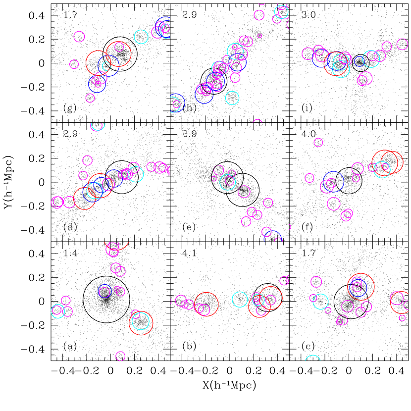
However, FOF results are very misleading. We compare the SO halos (as found by the BDM code) with the FOF halos found using . For halos with more than 100 particles both algorithms find essentially the same distinct halos, but FOF typically assigns larger masses to the same halos. The right panel in Figure 18 illustrates the point. There is a large variety of situations. We typically find that when there is a well-defined halo center and the halo dominates its environment, both the FOF and the SO masses are reasonably consistent (e.g., panel (a)). However, FOF has a tendency to link fragments of long filaments. In such cases the formal center of the FOF halo may not even be found in a large halo. Surprisingly, there are many of those long filaments at the high redshifts.


Figure 19 presents statistics for the ratios of FOF and SO masses. Left panels show the most massive 17000 halos with SO masses larger than at . There is a large spread of masses and on average FOF masses are 1.4 times larger than the SO counterparts. We made the same analysis for the most massive 10000 halos with the SO masses larger than at using for FOF. Remarkably, both halofinders produce similar results - a big contrast with high redshifts. Overall, there is a small offset in the mass ratios with SO producing 1.05 times larger masses. However, the difference is remarkably small.
Thus, as we stated in §4, FOF halo masses are similar to SO ones at low redshifts, but systematically larger at high redshifts.