Integrable discretizations for the short wave model of the Camassa-Holm equation

Abstract

The link between the short wave model of the Camassa-Holm equation (SCHE) and bilinear equations of the two-dimensional Toda lattice (2DTL) is clarified. The parametric form of $N$-cuspon solution of the SCHE in Casorati determinant is then given. Based on the above finding, integrable semi-discrete and full-discrete analogues of the SCHE are constructed. The determinant solutions of both semi-discrete and fully discrete analogues of the SCHE are also presented.

To be submitted to : J. Phys. A: Math. Gen.

1 Introduction

In the present paper, we consider integrable discretizations of the nonlinear partial differential equation

$$w_{TXX}-2\kappa^{2}w_{X}+2w_{X}w_{XX}+ww_{XXX}=0,$$ (1)

which belongs to the Harry-Dym hierarchy [1, 2, 3]. Here $\kappa$ is a real parameter and, as shown subsequently, can be normalized by the scaling transformation when $\kappa\neq 0$. A connection between Eq.(1) and the sinh-Gordon equation was established in [4]. When $\kappa=0$, Eq.(1) is called the Hunter-Saxton equation and is derived as a model for weakly nonlinear orientation waves in massive nematic liquid crystals [5]. The Lax pair and bi-Hamiltonian structure were discussed by Hunter and Zheng [6]. The dissipative and dispersive weak solutions were discussed in details by the same authors [7, 8].

Equation (1) can be viewed as a short-wave model of the Camassa-Holm equation [9]

$$w_{T}+2\kappa^{2}w_{X}-w_{TXX}+3ww_{X}=2w_{X}w_{XX}+ww_{XXX}\,.$$ (2)

Following the procedure in [10, 11, 12], we introduce the time and space variables ${\tilde{T}}$ and ${\tilde{X}}$

$${\tilde{T}}=\epsilon T\,,\quad{\tilde{X}}=\epsilon^{-1}X\,,$$

where $\epsilon$ is a small parameter. Then $w$ is expanded as $w=\epsilon^{2}(w_{0}+\epsilon w_{1}+\cdots)$ with $w_{i}$ ($i=0,1,\cdots$) being functions of ${\tilde{T}}$ and ${\tilde{X}}$. At the lowest order in $\epsilon$, we obtain

$$w_{0,{\tilde{T}}{\tilde{X}}{\tilde{X}}}-2\kappa^{2}w_{0,{\tilde{X}}}+2w_{0,{\tilde{X}}}w_{0,{\tilde{X}}{\tilde{X}}}+w_{0}w_{0,{\tilde{X}}{\tilde{X}}{\tilde{X}}}=0\,,$$ (3)

which is exactly Eq.(1) after writing back into the original variables. Based on this fact, Matsuno obtained the $N$-cuspon solution of Eq.(1) by taking the short-wave limit on the $N$-soliton solution of the Camassa-Holm equation [13, 14].

Note that the parameter $\kappa$ of Eq.(1) can be normalized to $1$ under the transformation

$$x=\kappa X\,,\quad t=\kappa T\,,$$

which leads to

$$w_{txx}-2w_{x}+2w_{x}w_{xx}+ww_{xxx}=0\,.$$ (4)

We call Eq.(4) the short wave model of the Camassa-Holm equation (SCHE). Without loss of generality, we will focus on Eq. (4) and its integrable discretizations, since the solution of Eq.(1) with arbitrary nonzero $\kappa$, its integrable discretizations and the corresponding solutions can be recovered through the above transformation.

The reminder of the present paper is organized as follows. In section 2, we reveal a connection between the SCHE and the bilinear form two-dimensional Toda-lattice (2DTL) equations. The parametric form of $N$-cuspon solution expressed by the Casorti determinant is given, which is consistent with the solution given in [13]. Based on this fact, we propose an integrable semi-discrete analogue of the SCHE in section 3, and further its integrable full-discrete analogue in section 4. The concluding remark is given in section 5.

2 The connection with 2DTL equations, and $N$-cuspon solution in determinant form

2.1 The link of the SCHE with the two-reduction of 2DTL equations

In this section, we will show that the SCHE can be derived from the bilinear form of two-dimensional Toda lattice (2DTL) equations

$$-\left(\frac{1}{2}D_{-1}D_{1}-1\right)\tau_{n}\cdot\tau_{n}=\tau_{n+1}\tau_{n-1}\,,$$ (5)

where $D_{x}$ is the Hirota $D$-derivative defined as

$$D_{x}^{n}f\cdot g=\left(\frac{\partial}{\partial x}-\frac{\partial}{\partial y}\right)^{n}f(x)g(y)|_{y=x}\,,$$

and $D_{-1}$ and $D_{1}$ represent the Hirota $D$ derivatives with respect to variables $x_{-1}$ and $x_{1}$, respectively.

It is shown that the $N$-soliton solution of the 2DTL equations (5) can be expressed as the Casorati determinant [16, 17]

$$\tau_{n}=\left|\psi_{i}^{(n+j-1)}(x_{1},x_{-1})\right|_{1\leq i,j\leq N}=\left|\matrix{\psi_{1}^{(n)}&\psi_{1}^{(n+1)}&\cdots&\psi_{1}^{(n+N-1)}\cr\psi_{2}^{(n)}&\psi_{2}^{(n+1)}&\cdots&\psi_{2}^{(n+N-1)}\cr\vdots&\vdots&\ddots&\vdots\cr\psi_{N}^{(n)}&\psi_{N}^{(n+1)}&\cdots&\psi_{N}^{(n+N-1)}}\right|\,,$$ (6)

with $\psi_{i}^{(n)}$ satisfying the following dispersion relations:

$$\frac{\partial\psi_{i}^{(n)}}{\partial x_{-1}}=\psi_{i}^{(n-1)},\qquad\frac{\partial\psi_{i}^{(n)}}{\partial x_{1}}=\psi_{i}^{(n+1)}\,.$$

A particular choice of $\psi_{i}^{(n)}$

$$\psi_{i}^{(n)}=a_{i,1}p_{i}^{n}e^{{p_{i}}^{-1}x_{-1}+p_{i}x_{1}+\eta_{0i}}+a_{i,2}q_{i}^{n}e^{{q_{i}}^{-1}x_{-1}+q_{i}x_{1}+\eta^{\prime}_{0i}}\,,$$ (7)

automatically satisfies the above dispersion relations.

Applying the two-reduction $\tau_{n-1}=(\prod_{i=1}^{N}p^{2}_{i})^{-1}\tau_{n+1}$, i.e., enforcing $p_{i}=-q_{i}$, $i=1,\cdots,N$, we get

$$-\left(\frac{1}{2}D_{-1}D_{1}-1\right)\tau_{n}\cdot\tau_{n}=\tau^{2}_{n+1}\,,$$ (8)

where the gauge transformation $\tau_{n}\to(\prod_{i=1}^{N}p_{i})^{n}\tau_{n}$ is used. Letting $\tau_{0}=f$, $\tau_{1}=g$ and $x_{-1}=s$, $x_{1}=y$, the above bilinear equation (8) takes the following form:

$$-\left(\frac{1}{2}D_{s}D_{y}-1\right)f\cdot f=g^{2}\,,$$ (9)

$$-\left(\frac{1}{2}D_{s}D_{y}-1\right)g\cdot g=f^{2}\,.$$ (10)

Introducing $u={g}/{f}$, Eqs.(9) and (10) can be converted into

$$-(\ln f)_{ys}+1 = u^{2}\,,$$ (11)

$$-(\ln g)_{ys}+1 = u^{-2}\,.$$ (12)

Subtracting Eq.(12) from Eq.(11), one obtains

$$\frac{\rho}{2}(\ln\rho)_{ys}+1=\rho^{2}\,,$$ (13)

by letting $\rho=u^{2}$.

Introducing the dependent variable transformation

$$w=-2(\ln g)_{ss}\,,$$

it then follows

$$\frac{1}{2}w_{y}=-\frac{\rho_{s}}{\rho^{2}}\,,$$

or

$$(\ln\rho)_{s}=-\frac{\rho}{2}w_{y}\,,$$ (14)

by differentiating Eq.(12) with respect to $s$.

In view of Eq.(14), Eq.(13) becomes

$$-\frac{\rho}{2}\left(\frac{\rho}{2}w_{y}\right)_{y}+1=\rho^{2}\,.$$ (15)

Introducing the hodograph transformation

$$\left\{\begin{array}[]{l}x=2y-2(\ln g)_{s}\,,\\ t=s\,,\end{array}\right.$$

and referring to Eq.(12), we have

$$\frac{\partial x}{\partial y}=2-2\left(\ln g\right)_{ys}=\frac{2}{\rho}\,,\qquad\frac{\partial x}{\partial s}=-2(\ln g)_{ss}=w\,,$$

which implies

$$\left\{\begin{array}[]{l}\displaystyle\partial_{y}=\frac{2}{\rho}\partial_{x}\,,\\[5.0pt] \partial_{s}=\partial_{t}+w\partial_{x}\,.\end{array}\right.$$

Thus, Eqs.(14) and (15) can be cast into

$$\left\{\begin{array}[]{l}\displaystyle(\partial_{t}+w\partial_{x})\ln\rho=-w_{x}\,,\\[5.0pt] \displaystyle-w_{xx}+1=\rho^{2}\,.\end{array}\right.$$ (16)

By eliminating $\rho$, we arrive at

$$(\partial_{t}+w\partial_{x})\ln\left(-w_{xx}+1\right)=-2w_{x}\,,$$

or

$$(\partial_{t}+w\partial_{x})w_{xx}-2w_{x}\left(1-w_{xx}\right)=0\,,$$

which is actually the SCHE (4).

2.2 The $N$-cuspon solution of the SCHE

Based on the link of the SCHE with the two-reduction of 2DTL equations, the $N$-cuspon solution of the SCHE (4) is given as follows:

$$w=-2(\ln g)_{ss}\,,$$

$$\left\{\begin{array}[]{l}x=2y-2(\ln g)_{s}\,,\\ t=s\,,\end{array}\right.$$

$$g=\left|\psi_{i}^{(j)}(y,s)\right|_{1\leq i,j\leq N}\,\,,$$

$$\psi_{i}^{(j)}=a_{i,1}p_{i}^{j}e^{{p_{i}}^{-1}s+p_{i}y+\eta_{0i}}+a_{i,2}(-p_{i})^{j}e^{-{p_{i}}^{-1}s-p_{i}y+\eta^{\prime}_{0i}}\,.$$ (17)

Moreover, the $N$-cuspon solution of the SCHE (1) with non-zero $\kappa$ is given as follows:

$$w(y,T)=-2(\ln g)_{ss},$$ (18)

$$\left\{\begin{array}[]{l}X=\frac{2y}{\kappa}-\frac{2}{\kappa}(\ln g)_{s},\\ T=\frac{s}{\kappa}\,,\end{array}\right.$$ (19)

where

$$g=\left|\psi_{i}^{(j)}(y,s)\right|_{1\leq i,j\leq N}\,,$$

with

$$\psi_{i}^{(n)}=a_{i,1}p_{i}^{n}e^{p_{i}y+s/p_{i}+\eta_{i0}}+a_{i,2}(-p_{i})^{n}e^{-p_{i}y-s/p_{i}+\eta^{\prime}_{i0}}\,.$$

We remark here that to assure the regularity of the solution, the $\tau$-function is required to be positive definite. In what follows, we list the one-cuspon and two-cuspon solutions. For $N=1$, the $\tau$-function is

$$g=1+e^{2p_{1}(y+\kappa T/p^{2}_{1}+y_{0})}\,,$$

by choosing $a_{1,1}/a_{1,2}=-1$, which yields the one-cuspon solution

$$w(y,T)=-\frac{2}{p^{2}_{1}}{\mbox{sech}}^{2}\left[p_{1}(y+\kappa T/p^{2}_{1}+y_{0})\right]\,,$$

$$X=\frac{2y}{\kappa}-\frac{2}{\kappa p_{1}}\left\{1+\tanh\left[p_{1}(y+\kappa T/p^{2}_{1}+y_{0})\right]\right\}\,.$$

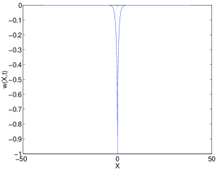
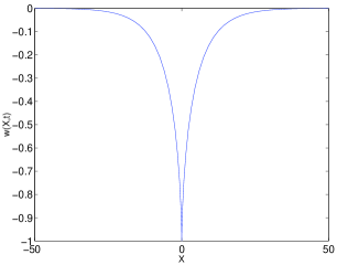
The profiles of one-cuspon with $\kappa=1.0$ and $\kappa=0.1$ are plotted in Fig. 1.

 

(a)(b)

Figure 1: Plots for one-cuspon solution for $p_{1}=\sqrt{2}$ and different $\kappa$: (a) $\kappa=1.0$; (b) $\kappa=0.1$.

The $\tau$-function corresponding to the two-cuspon solution is

$$g=1+e^{\theta_{1}}+e^{\theta_{2}}+\left(\frac{p_{1}-p_{2}}{p_{1}-p_{2}}\right)^{2}e^{\theta_{1}+\theta_{2}}\,,$$

with

$$\theta_{i}=2p_{i}(y+\kappa T/p^{2}_{i}+y_{i0}),\ i=1,2\,.$$

Here $a_{1,1}/a_{1,2}=-1$ and $a_{2,1}/a_{2,2}=1$ are chosen to assure the regularity of the solution.

3 Integrable semi-discretization of the SCHE

Based on the link of the SCHE with the two-reduction of 2DTL equations clarified in the previous section, we attempt to construct the integrable semi-discrete analogue of the SCHE.

Consider a Casorati determinant

$$\tau_{n}(k)=\left|\psi_{i}^{(n+j-1)}(k)\right|_{1\leq i,j\leq N}=\left|\matrix{\psi_{1}^{(n)}(k)&\psi_{1}^{(n+1)}(k)&\cdots&\psi_{1}^{(n+N-1)}(k)\cr\psi_{2}^{(n)}(k)&\psi_{2}^{(n+1)}(k)&\cdots&\psi_{2}^{(n+N-1)}(k)\cr\vdots&\vdots&\ddots&\vdots\cr\psi_{N}^{(n)}(k)&\psi_{N}^{(n+1)}(k)&\cdots&\psi_{N}^{(n+N-1)}(k)}\right|\,,$$

with $\psi_{i}^{(n)}$ satisfies the following dispersion relations

$$\Delta_{k}\psi_{i}^{(n)}=\psi_{i}^{(n+1)}\,,$$ (20)

$$\partial_{s}\psi_{i}^{(n)}=\psi_{i}^{(n-1)}\,,$$ (21)

where $\Delta_{k}$ is defined as $\Delta_{k}\psi(k)=\frac{\psi(k)-\psi(k-1)}{a}$. In particular, we can choose $\psi_{i}^{(n)}$ as

$$\psi_{i}^{(n)}(k)=p_{i}^{n}(1-ap_{i})^{-k}e^{\xi_{i}}+q_{i}^{n}(1-aq_{i})^{-k}e^{\eta_{i}}\,,$$

$$\xi_{i}=\frac{1}{p_{i}}s+\xi_{i0}\,,\quad\eta_{i}=\frac{1}{q_{i}}s+\eta_{i0}\,,$$

which automatically satisfies the dispersion relations (20) and (21). The above Casorati determinant satisfies the bilinear form of the semi-discrete 2DTL equation (the Bäcklund transformation of the bilinear equation of the 2DTL equation) [17, 18]

$$\left(\frac{1}{a}D_{s}-1\right)\tau_{n}(k+1)\cdot\tau_{n}(k)+\tau_{n+1}(k+1)\tau_{n-1}(k)=0\,.$$ (22)

Applying a two-reduction condition $p_{i}=-q_{i}$, $i=1,\cdots,N$, which implies $\tau_{n-1}\Bumpeq\tau_{n+1}$, we obtain

$$-\left(\frac{1}{a}D_{s}-1\right)f_{k+1}\cdot f_{k}=g_{k+1}g_{k}\,,$$ (23)

$$-\left(\frac{1}{a}D_{s}-1\right)g_{k+1}\cdot g_{k}=f_{k+1}g_{k}\,,$$ (24)

by letting $\tau_{0}(k)=f_{k}$, $\tau_{1}(k)=g_{k}$.

Letting $u_{k}=g_{k}/f_{k}$, Eqs.(23) and (24) are equivalent to

$$-\frac{1}{a}\left(\ln\frac{f_{k+1}}{f_{k}}\right)_{s}+1 = u_{k+1}u_{k}\,,$$ (25)

$$-\frac{1}{a}\left(\ln\frac{g_{k+1}}{g_{k}}\right)_{s}+1 = u^{-1}_{k+1}u^{-1}_{k}\,.$$ (26)

Subtracting Eq.(26) from Eq.(25), one obtains

$$\frac{u_{k+1}u_{k}}{a}\left(\ln\frac{u_{k+1}}{u_{k}}\right)_{s}+1=u^{2}_{k+1}u^{2}_{k}\,.$$ (27)

Introducing the discrete analogue of hodograph transformation

$$x_{k}=2ka-2(\ln g_{k})_{s}\,,$$

and

$$\delta_{k}=x_{k+1}-x_{k}=2a-2\left(\ln\frac{g_{k+1}}{g_{k}}\right)_{s}\,.$$

It then follows from Eq.(26)

$$\delta_{k}=\frac{2a}{u_{k+1}u_{k}}\,,$$

or

$$\rho_{k+1}\rho_{k}=\frac{4a^{2}}{\delta_{k}^{2}}\,,$$ (28)

by assuming $\rho_{k}=u^{2}_{k}$.

Introducing the dependent variable transformation

$$w_{k}=-2(\ln g_{k})_{ss}\,,$$

Eq.(27) becomes

$$\frac{1}{\delta_{k}}\left(\ln\frac{\rho_{k+1}}{\rho_{k}}\right)_{s}+1-\frac{4a^{2}}{\delta_{k}^{2}}=0\,.$$ (29)

Differentiating Eq.(26) with respect to $s$, we have

$$\frac{1}{2a}(w_{k+1}-w_{k})=-\frac{1}{u_{k+1}u_{k}}\left(\ln u_{k+1}u_{k}\right)_{s}=-\frac{1}{2u_{k+1}u_{k}}\left(\ln\rho_{k+1}\rho_{k}\right)_{s}\,,$$

or

$$(\ln\rho_{k+1}\rho_{k})_{s}=-\frac{2}{\delta_{k}}(w_{k+1}-w_{k})\,.$$ (30)

Eliminating $\rho_{k}$ and $\rho_{k+1}$ from Eqs.(29) and (30), we obtain

$$\frac{1}{\delta_{k}}(w_{k+1}-w_{k})-\frac{1}{\delta_{k-1}}(w_{k}-w_{k-1})=\frac{1}{2}(\delta_{k}+\delta_{k-1})-2a^{2}\left(\frac{1}{\delta_{k}}+\frac{1}{\delta_{k-1}}\right)\,,$$ (31)

or

$$\Delta^{2}w_{k}=\frac{1}{\delta_{k}}M\left(\delta_{k}-\frac{4a^{2}}{\delta_{k}}\right)\,,$$ (32)

by defining a difference operator $\Delta$ and an average operator $M$ as follows

$$\Delta F_{k}=\frac{F_{k+1}-F_{k}}{\delta_{k}}\,,\quad MF_{k}=\frac{F_{k+1}+F_{k}}{2}\,.$$

Furthermore, a substitution of Eq.(28) into Eq. (30) leads to

$$\frac{d\delta_{k}}{ds}=w_{k+1}-w_{k}\,.$$ (33)

Equations (31) and (33) constitute the semi-discrete analogue of the SCHE.

Next, let us show that in the continuous limit, $a\to 0$ ($\delta_{k}\to 0$), the proposed semi-discrete SCHE recovers the continuous SCHE. To this end, Eqs.(31) and (33) are rewritten as

$$\left\{\begin{array}[]{l}\displaystyle\frac{-2}{\delta_{k}+\delta_{k-1}}\left(\Delta w_{k}-\Delta w_{k-1}\right)+1=\frac{4a^{2}}{\delta_{k}\delta_{k-1}}\,,\\[15.0pt] \displaystyle\partial_{s}\delta_{k}=w_{k+1}-w_{k}\,.\end{array}\right.$$

By taking logarithmic derivative of the first equation, we get

$$\frac{\displaystyle\partial_{s}\left\{\frac{-2}{\delta_{k}+\delta_{k-1}}\left(\Delta w_{k}-\Delta w_{k-1}\right)+1\right\}}{\displaystyle\frac{-2}{\delta_{k}+\delta_{k-1}}\left(\Delta w_{k}-\Delta w_{k-1}\right)+1}=-\frac{\partial_{s}\delta_{k}}{\delta_{k}}-\frac{\partial_{s}\delta_{k-1}}{\delta_{k-1}}\,.$$

The dependent variable $w$ is regarded as a function of $x$ and $t$, where $x$ is the space coordinate of the $k$-th lattice point and $t$ is the time, defined by

$$x_{k}=x_{0}+\sum_{j=0}^{k-1}\delta_{j}\,,\qquad t=s\,.$$

In the continuous limit, $a\to 0$ ($\delta_{k}\to 0$), we have

$$\frac{\partial_{s}\delta_{k}}{\delta_{k}}=\frac{w_{k+1}-w_{k}}{\delta_{k}}\to w_{x}\,,\quad\frac{\partial_{s}\delta_{k-1}}{\delta_{k-1}}=\frac{w_{k}-w_{k-1}}{\delta_{k-1}}\to w_{x}\,,$$

$$\frac{2}{\delta_{k}+\delta_{k-1}}\left(\Delta w_{k}-\Delta w_{k-1}\right)\to w_{xx}\,,$$

$$\frac{\partial x_{k}}{\partial s}=\frac{\partial x_{0}}{\partial s}+\sum_{j=0}^{k-1}\frac{\partial\delta_{j}}{\partial s}=\frac{\partial x_{0}}{\partial s}+\sum_{j=0}^{k-1}(w_{j+1}-w_{j})\to w\,,$$

$$\partial_{s}=\partial_{t}+\frac{\partial x}{\partial s}\partial_{x}\to\partial_{t}+w\partial_{x}\,,$$

where the origin of space coordinate $x_{0}$ is taken so that $\displaystyle\frac{\partial x_{0}}{\partial s}$ cancels $w_{0}$. Thus the above semi-discrete SCHE converges to

$$\frac{(\partial_{t}+w\partial_{x})(-w_{xx}+1)}{\displaystyle-w_{xx}+1}=-2w_{x}\,,$$

or

$$(\partial_{t}+w\partial_{x})w_{xx}=2w_{x}\left({\displaystyle-w_{xx}+1}\right)\,,$$ (34)

which is nothing but the SCHE (4).

In summary, the semi-discrete analogue of the SCHE and its determinant solution are given as follows:
The semi-discrete analogue of the SCHE

$$\left\{\begin{array}[]{l}\displaystyle\frac{1}{\delta_{k}}(w_{k+1}-w_{k})-\frac{1}{\delta_{k-1}}(w_{k}-w_{k-1})=\frac{1}{2}(\delta_{k}+\delta_{k-1})-2a^{2}\left(\frac{1}{\delta_{k}}+\frac{1}{\delta_{k-1}}\right)\,,\\[15.0pt] \displaystyle\frac{d\delta_{k}}{dt}=w_{k+1}-w_{k}\,.\end{array}\right.$$ (35)

The determinant solution of the semi-discrete SCHE

$$w_{k}=-2(\ln g_{k})_{ss}\,,$$

$$\delta_{k}=x_{k+1}-x_{k}=2a\frac{f_{k+1}f_{k}}{g_{k+1}g_{k}}\,,$$

$$\left\{\begin{array}[]{l}x_{k}=2ka-2(\ln g_{k})_{s}\,,\\ t=s\,,\end{array}\right.$$

$$g_{k}=\left|\psi_{i}^{(j)}(k)\right|_{1\leq i,j\leq N}\,,\quad f_{k}=\left|\psi_{i}^{(j-1)}(k)\right|_{1\leq i,j\leq N}\,,$$

$$\psi_{i}^{(j)}(k)=a_{i,1}p_{i}^{j}(1-ap_{i})^{-k}e^{{p_{i}}^{-1}s+\eta_{0i}}+a_{i,2}(-p_{i})^{j}(1+ap_{i})^{-k}e^{-{p_{i}}^{-1}s+\eta^{\prime}_{0i}}\,.$$ (36)

Introducing new independent variables $X_{k}=x_{k}/\kappa$ and $T=t/\kappa$, we can include the parameter $\kappa$ in the semi-discrete SCHE (35)

$$\left\{\begin{array}[]{l}\displaystyle\frac{1}{\delta_{k}}(w_{k+1}-w_{k})-\frac{1}{\delta_{k-1}}(w_{k}-w_{k-1})=\frac{1}{2\kappa^{2}}(\delta_{k}+\delta_{k-1})-2a^{2}\left(\frac{1}{\delta_{k}}+\frac{1}{\delta_{k-1}}\right)\,,\\[15.0pt] \displaystyle\frac{d\delta_{k}}{dT}=w_{k+1}-w_{k}\,,\end{array}\right.$$ (37)

where $\delta_{k}=X_{k+1}-X_{k}$ and $s=\kappa T$. This is the semi-discrete analogue of the SCHE (1).

The $N$-cuspon solution of the semi-discrete SCHE (37) with the parameter $\kappa$ is given by

$$w_{k}=-2(\ln g_{k})_{ss}\,,$$

$$\delta_{k}=X_{k+1}-X_{k}=\frac{2a}{\kappa}\frac{f_{k+1}f_{k}}{g_{k+1}g_{k}}\,,$$

$$\left\{\begin{array}[]{l}X_{k}=\frac{2ka}{\kappa}-\frac{2}{\kappa}(\ln g_{k})_{s}\,,\\ T=\frac{s}{\kappa}\,,\end{array}\right.$$

$$g_{k}=\left|\psi_{i}^{(j)}(k)\right|_{1\leq i,j\leq N}\,,\quad f_{k}=\left|\psi_{i}^{(j-1)}(k)\right|_{1\leq i,j\leq N}\,,$$

$$\psi_{i}^{(j)}(k)=a_{i,1}p_{i}^{j}(1-ap_{i})^{-k}e^{{p_{i}}^{-1}s+\eta_{0i}}+a_{i,2}(-p_{i})^{j}(1+ap_{i})^{-k}e^{-{p_{i}}^{-1}s+\eta^{\prime}_{0i}}\,.$$ (38)

4 Full-discretization of the SCHE

In much the same way of finding the semi-discrete analogue of the SCHE, we seek for its full-discrete analogue and in the process we arrive at its $N$-cuspon solution.

Consider the following Casorati determinant

$$\tau_{n}(k,l)=\left|\psi_{i}^{(n+j-1)}(k,l)\right|_{1\leq i,j\leq N}\,,$$ (39)

where

$$\psi_{i}^{(n)}(k,l)=a_{i,1}p_{i}^{n}(1-ap_{i})^{-k}\left(1-b{p_{i}}^{-1}\right)^{-l}e^{\xi_{i}}+a_{i,2}q_{i}^{n}(1-aq_{i})^{-k}\left(1-b{q_{i}}^{-1}\right)^{-l}e^{\eta_{i}}\,,$$

with

$$\xi_{i}={p_{i}}^{-1}s+\xi_{i0}\,,\quad\eta_{i}={q_{i}}^{-1}s+\eta_{i0}\,.$$

It is known that the above determinant satisfies bilinear equations [18]

$$\left(\frac{1}{a}D_{s}-1\right)\tau_{n}(k+1,l)\cdot\tau_{n}(k,l)+\tau_{n+1}(k+1,l)\tau_{n-1}(k,l)=0\,,$$ (40)

and

$$(bD_{s}-1)\tau_{n}(k,l+1)\cdot\tau_{n+1}(k,l)+\tau_{n}(k,l)\tau_{n+1}(k,l+1)=0\,.$$ (41)

Here $a,b$ are mesh sizes for space and time variables, respectively.

Applying the two-reduction $\tau_{n-1}=(\prod_{i=1}^{N}p^{2}_{i})^{-1}\tau_{n+1}$, i.e., enforcing $p_{i}=-q_{i}$, $i=1,\cdots,N$, and letting $\tau_{0}(k,l)=f_{k,l}$, $\tau_{1}(k,l)=g_{k,l}$, the above bilinear equations take the following form:

$$\left(\frac{1}{a}D_{s}-1\right)f_{k+1,l}\cdot f_{k,l}+{g}_{k+1,l}{g}_{k,l}=0\,,$$ (42)

$$\left(\frac{1}{a}D_{s}-1\right){g}_{k+1,l}\cdot{g}_{k,l}+{f}_{k+1,l}{f}_{k,l}=0\,,$$ (43)

$$(bD_{s}-1)f_{k,l+1}\cdot{g}_{k,l}+f_{k,l}{g}_{k,l+1}=0\,,$$ (44)

$$(bD_{s}-1){g}_{k,l+1}\cdot f_{k,l}+{g}_{k,l}f_{k,l+1}=0\,,$$ (45)

where the gauge transformation $\tau_{n}\to(\prod_{i=1}^{N}p_{i})^{n}\tau_{n}$ is used. It is readily shown that the above equations are equivalent to

$$\frac{1}{a}\left(\ln\frac{f_{k+1,l}}{f_{k,l}}\right)_{s}=1-\frac{{g}_{k+1,l}{g}_{k,l}}{f_{k+1,l}f_{k,l}}\,,$$ (46)

$$\frac{1}{a}\left(\ln\frac{{g}_{k+1,l}}{{g}_{k,l}}\right)_{s}=1-\frac{f_{k+1,l}f_{k,l}}{{g}_{k+1,l}{g}_{k,l}}\,,$$ (47)

$$b\left(\ln\frac{f_{k,l+1}}{{g}_{k,l}}\right)_{s}=1-\frac{f_{k,l}{g}_{k,l+1}}{f_{k,l+1}{g}_{k,l}}\,,$$ (48)

$$b\left(\ln\frac{{g}_{k,l+1}}{f_{k,l}}\right)_{s}=1-\frac{{g}_{k,l}f_{k,l+1}}{{g}_{k,l+1}f_{k,l}}\,.$$ (49)

We introduce a dependent variable transformation

$$w_{k,l}=-2\left(\ln{g_{k,l}}\right)_{ss}\,,$$ (50)

and a discrete hodograph transformation

$$x_{k,l}=2ka-2(\ln g_{k,l})_{s}\,,$$ (51)

then the mesh

$$\delta_{k,l}=x_{k+1,l}-x_{k,l}=2a-2\left(\ln{\frac{g_{k+1,l}}{g_{k,l}}}\right)_{s}\,$$ (52)

is naturally defined. It then follows

$$\left(\ln{\frac{g_{k+1,l}}{g_{k-1,l}}}\right)_{s}=2a-\frac{1}{2}\left(\delta_{k,l}+\delta_{k-1,l}\right)\,.$$ (53)

In view of Eq.(47), one obtains

$$\frac{f_{k+1,l}f_{k,l}}{{g}_{k+1,l}{g}_{k,l}}=\frac{\delta_{k,l}}{2a}\,.$$ (54)

A substitution into Eq.(46) yields

$$\left(\ln{\frac{f_{k+1,l}}{f_{k,l}}}\right)_{s}=a-\frac{2a^{2}}{\delta_{k,l}}\,,$$ (55)

it then follows

$$\left(\ln{\frac{f_{k+1,l}}{f_{k-1,l}}}\right)_{s}=2a-{2a^{2}}\left(\frac{1}{\delta_{k,l}}+\frac{1}{\delta_{k-1,l}}\right)\,.$$ (56)

Starting from an alternative form of Eq.(47)

$$2a-2\left(\ln\frac{{g}_{k+1,l}}{{g}_{k,l}}\right)_{s}=2a\frac{f_{k+1,l}f_{k,l}}{{g}_{k+1,l}{g}_{k,l}}\,,$$ (57)

we obtain

$$\frac{w_{k+1,l}-w_{k,l}}{\delta_{k,l}}=\frac{-2\left(\ln\frac{{g}_{k+1,l}}{{g}_{k,l}}\right)_{ss}}{2a-2\left(\ln\frac{{g}_{k+1,l}}{{g}_{k,l}}\right)_{s}}=\left(\ln\frac{f_{k+1,l}f_{k,l}}{{g}_{k+1,l}{g}_{k,l}}\right)_{s}\,,$$ (58)

by taking logarithmic derivative with respect to $s$. A shift from $k$ to $k-1$ gives

$$\frac{w_{k,l}-w_{k-1,l}}{\delta_{k-1,l}}=\left(\ln\frac{f_{k,l}f_{k-1,l}}{{g}_{k,l}{g}_{k-1,l}}\right)_{s}\,.$$ (59)

Subtracting Eq.(59) from Eq.(58), we obtain

$$\frac{w_{k+1,l}-w_{k,l}}{\delta_{k,l}}-\frac{w_{k,l}-w_{k-1,l}}{\delta_{k-1,l}}=\left(\ln{\frac{f_{k+1,l}}{f_{k-1,l}}}\right)_{s}-\left(\ln{\frac{g_{k+1,l}}{g_{k-1,l}}}\right)_{s}\,.$$ (60)

By using the relations (53) and (56), we finally arrive at

$$\frac{w_{k+1,l}-w_{k,l}}{\delta_{k,l}}-\frac{w_{k,l}-w_{k-1,l}}{\delta_{k-1,l}}-\frac{1}{2}\left(\delta_{k,l}+\delta_{k-1,l}\right)+{2a^{2}}\left(\frac{1}{\delta_{k,l}}+\frac{1}{\delta_{k-1,l}}\right)=0\,.$$ (61)

Similar to Eq.(32), Eq.(61) constitutes the first equation of the full-discretization of the SCHE, which can be cast into a simpler form:

$$\Delta^{2}w_{k,l}=\frac{1}{\delta_{k,l}}M\left(\delta_{k,l}-\frac{4a^{2}}{\delta_{k,l}}\right)\,.$$ (62)

Next, we seek for the second equation of the full-discretization. Recalling (46)–(49), one could obtain

$$\frac{x_{k+1,l+1}-x_{k,l+1}}{x_{k+1,l}-x_{k,l}}=\frac{2a-2\left(\ln\frac{{g}_{k+1,l+1}}{{g}_{k,l+1}}\right)_{s}}{2a-2\left(\ln\frac{{g}_{k+1,l}}{{g}_{k,l}}\right)_{s}}=\frac{\left(\ln\frac{{g}_{k+1,l+1}}{{f}_{k+1,l}}\right)_{s}-\frac{1}{b}}{\left(\ln\frac{{f}_{k,l+1}}{{g}_{k,l}}\right)_{s}-\frac{1}{b}}\,,$$ (63)

here a shift from $l$ to $l+1$ in (47) and a shift from $k$ to $k+1$ in (49) are employed.

From Eqs.(50), (55) and (58), one can find the following two relations

$$\left(\ln\frac{{g}_{k+1,l+1}}{{f}_{k+1,l}}\right)_{s}=-\frac{w_{k+1,l}-w_{k,l}-2a^{2}}{2\delta_{k,l}}+\frac{1}{4}\left(x_{k+1,l}+x_{k,l}-2x_{k+1,l+1}\right)\,,$$ (64)

$$\left(\ln\frac{{f}_{k,l+1}}{{g}_{k,l}}\right)_{s}=\frac{w_{k+1,l+1}-w_{k,l+1}+2a^{2}}{2\delta_{k,l+1}}-\frac{1}{4}\left(x_{k+1,l+1}+x_{k,l+1}-2x_{k,l}\right)\,,$$ (65)

after some tedious algebraic manipulations. Substituting these two relations into (63), we finally obtain the second equation of the fully discrete analogue of the SCHE

$$\frac{\delta_{k,l+1}-\delta_{k,l}}{b} + \frac{1}{4}\delta_{k,l+1}\left(x_{k+1,l+1}+x_{k,l+1}-2x_{k,l}\right)$$ (66)

$$+ \frac{1}{4}\delta_{k,l}\left(x_{k+1,l}+x_{k,l}-2x_{k+1,l+1}\right)$$

$$= \frac{1}{2}\left(w_{k+1,l+1}+w_{k+1,l}-w_{k,l+1}-w_{k,l}\right)\,.$$

Taking the continuous limit $b\to 0$ in time, we have

$$\frac{\delta_{k,l+1}-\delta_{k,l}}{b}\to\frac{d\delta_{k}}{ds}\,,$$

$$\delta_{k,l+1}\left(x_{k+1,l+1}+x_{k,l+1}-2x_{k,l}\right)\to 0\,,$$

$$\delta_{k,l+1}\delta_{k,l}\left(x_{k+1,l}+x_{k,l}-2x_{k+1,l+1}\right)\to 0\,,$$

and

$$\frac{1}{2}\left(w_{k+1,l+1}+w_{k+1,l}-w_{k,l+1}-w_{k,l}\right)\to w_{k+1}-w_{k}.$$

Therefore, one recovers exactly the second equation of the semi-discrete SCHE (33).

In summary, the fully discrete analogue of the SCHE and its determinant solution are given as follows:
The fully discrete analogue of the SCHE

$$\left\{\begin{array}[]{l}\displaystyle\frac{w_{k+1,l}-w_{k,l}}{\delta_{k,l}}-\frac{w_{k,l}-w_{k-1,l}}{\delta_{k-1,l}}-\frac{1}{2}\left(\delta_{k,l}+\delta_{k-1,l}\right)+{2a^{2}}\left(\frac{1}{\delta_{k,l}}+\frac{1}{\delta_{k-1,l}}\right)=0\,,\\[15.0pt] \displaystyle\frac{\delta_{k,l+1}-\delta_{k,l}}{b}+\frac{1}{4}\delta_{k,l+1}\left(x_{k+1,l+1}+x_{k,l+1}-2x_{k,l}\right)\\[15.0pt] \displaystyle\qquad+\frac{1}{4}\delta_{k,l}\left(x_{k+1,l}+x_{k,l}-2x_{k+1,l+1}\right)=\frac{1}{2}\left(w_{k+1,l+1}+w_{k+1,l}-w_{k,l+1}-w_{k,l}\right)\,.\end{array}\right.$$ (67)

The determinant solution of the fully discrete SCHE

$$w_{k,l}=-2(\ln g_{k,l})_{ss}=-2\frac{{\bar{h}_{k,l}}g_{k,l}-h_{k,l}^{2}}{g_{k,l}^{2}}\,,$$

$$x_{k,l}=2ka-2(\ln g_{k,l})_{s}=2ka-2\frac{h_{k,l}}{g_{k,l}}\,,$$

$$\delta_{k,l}=x_{k+1,l}-x_{k,l}=2a\frac{f_{k+1,l}f_{k,l}}{g_{k+1,l}g_{k,l}}\,,$$

$$g_{k,l}=\left|\psi_{i}^{(j)}(k,l)\right|_{1\leq i,j\leq N}\,,\quad f_{k,l}=\left|\psi_{i}^{(j-1)}(k,l)\right|_{1\leq i,j\leq N}\,,$$

$$h_{k,l}=\frac{\partial g_{k,l}}{\partial s}=\left|\matrix{\psi_{1}^{(0)}(k,l)&\psi_{1}^{(2)}(k,l)&\psi_{1}^{(3)}(k,l)&\cdots&\psi_{1}^{(N)}(k,l)\cr\psi_{2}^{(0)}(k,l)&\psi_{2}^{(2)}(k,l)&\psi_{2}^{(3)}(k,l)&\cdots&\psi_{2}^{(N)}(k,l)\cr\vdots&\vdots&\vdots&\ddots&\vdots\cr\psi_{N}^{(0)}(k,l)&\psi_{N}^{(2)}(k,l)&\psi_{N}^{(3)}(k,l)&\cdots&\psi_{N}^{(N)}(k,l)}\right|\,,$$

$${\bar{h}}_{k,l}=\frac{\partial^{2}g_{k,l}}{\partial s^{2}}=\left|\matrix{\psi_{1}^{(-1)}(k,l)&\psi_{1}^{(2)}(k,l)&\psi_{1}^{(3)}(k,l)&\cdots&\psi_{1}^{(N)}(k,l)\cr\psi_{2}^{(-1)}(k,l)&\psi_{2}^{(2)}(k,l)&\psi_{2}^{(3)}(k,l)&\cdots&\psi_{2}^{(N)}(k,l)\cr\vdots&\vdots&\vdots&\ddots&\vdots\cr\psi_{N}^{(-1)}(k,l)&\psi_{N}^{(2)}(k,l)&\psi_{N}^{(3)}(k,l)&\cdots&\psi_{N}^{(N)}(k,l)}\right|$$

$$\qquad+\left|\matrix{\psi_{1}^{(0)}(k,l)&\psi_{1}^{(1)}(k,l)&\psi_{1}^{(3)}(k,l)&\cdots&\psi_{1}^{(N)}(k,l)\cr\psi_{2}^{(0)}(k,l)&\psi_{2}^{(1)}(k,l)&\psi_{2}^{(3)}(k,l)&\cdots&\psi_{2}^{(N)}(k,l)\cr\vdots&\vdots&\vdots&\ddots&\vdots\cr\psi_{N}^{(0)}(k,l)&\psi_{N}^{(1)}(k,l)&\psi_{N}^{(3)}(k,l)&\cdots&\psi_{N}^{(N)}(k,l)}\right|\,,$$

$$\psi_{i}^{(j)}(k,l)=a_{i,1}p_{i}^{j}(1-ap_{i})^{-k}\left(1-b{p_{i}}^{-1}\right)^{-l}e^{\xi_{i}}+a_{i,2}(-p_{i})^{j}(1+ap_{i})^{-k}\left(1+b{p_{i}}^{-1}\right)^{-l}e^{\eta_{i}}\,,$$

$$\xi_{i}={p_{i}}^{-1}s+\xi_{i0}\,,\quad\eta_{i}=-{p_{i}}^{-1}s+\eta_{i0}\,.$$ (68)

Note that $s$ is an auxiliary parameter. By virtue of $s$, $h_{k,l}$ and ${\bar{h}}_{k,l}$ can be expressed as $h_{k,l}=\partial_{s}g_{k,l}$ and ${\bar{h}}_{k,l}=\partial^{2}_{s}g_{k,l}$, respectively, because the auxiliary parameter $s$ works on elements of the above determinant by $\partial_{s}\psi_{i}^{(n)}(k,l)=\psi_{i}^{(n-1)}(k,l)$.

Introducing new independent variables $X_{k,l}=x_{k,l}/\kappa$ and $\tilde{b}=b/\kappa$, we can include the parameter $\kappa$ in the full-discrete SCHE (67):

$$\left\{\begin{array}[]{l}\displaystyle\frac{w_{k+1,l}-w_{k,l}}{\delta_{k,l}}-\frac{w_{k,l}-w_{k-1,l}}{\delta_{k-1,l}}-\frac{1}{2\kappa^{2}}\left(\delta_{k,l}+\delta_{k-1,l}\right)+{2a^{2}}\left(\frac{1}{\delta_{k,l}}+\frac{1}{\delta_{k-1,l}}\right)=0\,,\\[15.0pt] \displaystyle\frac{\delta_{k,l+1}-\delta_{k,l}}{\tilde{b}}+\frac{1}{4\kappa^{2}}\delta_{k,l+1}\left(X_{k+1,l+1}+X_{k,l+1}-2X_{k,l}\right)\\[15.0pt] \displaystyle\qquad+\frac{1}{4\kappa^{2}}\delta_{k,l}\left(X_{k+1,l}+X_{k,l}-2X_{k+1,l+1}\right)=\frac{1}{2}\left(w_{k+1,l+1}+w_{k+1,l}-w_{k,l+1}-w_{k,l}\right)\,.\end{array}\right.$$ (69)

Similarly, the $N$-cuspon solution of the full-discrete SCHE (69) with the parameter $\kappa$ is given as follows:

$$w_{k,l}=-2(\ln g_{k,l})_{ss}=-{2}\frac{{\bar{h}_{k,l}}g_{k,l}-h_{k,l}^{2}}{g_{k,l}^{2}}\,,$$

$$X_{k,l}=\frac{2ka}{\kappa}-\frac{2}{\kappa}(\ln g_{k,l})_{s}=\frac{2ka}{\kappa}-\frac{2}{\kappa}\frac{h_{k,l}}{g_{k,l}}\,,$$

$$\delta_{k,l}=X_{k+1,l}-X_{k,l}=\frac{2a}{\kappa}\frac{f_{k+1,l}f_{k,l}}{g_{k+1,l}g_{k,l}}\,,$$

$$g_{k,l}=\left|\psi_{i}^{(j)}(k,l)\right|_{1\leq i,j\leq N}\,,\quad f_{k,l}=\left|\psi_{i}^{(j-1)}(k,l)\right|_{1\leq i,j\leq N}\,,$$

$$h_{k,l}=\frac{\partial g_{k,l}}{\partial s}=\frac{1}{\kappa}\left|\matrix{\psi_{1}^{(0)}(k,l)&\psi_{1}^{(2)}(k,l)&\psi_{1}^{(3)}(k,l)&\cdots&\psi_{1}^{(N)}(k,l)\cr\psi_{2}^{(0)}(k,l)&\psi_{2}^{(2)}(k,l)&\psi_{2}^{(3)}(k,l)&\cdots&\psi_{2}^{(N)}(k,l)\cr\vdots&\vdots&\vdots&\ddots&\vdots\cr\psi_{N}^{(0)}(k,l)&\psi_{N}^{(2)}(k,l)&\psi_{N}^{(3)}(k,l)&\cdots&\psi_{N}^{(N)}(k,l)}\right|\,,$$

$${\bar{h}}_{k,l}=\frac{\partial^{2}g_{k,l}}{\partial s^{2}}=\frac{1}{\kappa^{2}}\left|\matrix{\psi_{1}^{(-1)}(k,l)&\psi_{1}^{(2)}(k,l)&\psi_{1}^{(3)}(k,l)&\cdots&\psi_{1}^{(N)}(k,l)\cr\psi_{2}^{(-1)}(k,l)&\psi_{2}^{(2)}(k,l)&\psi_{2}^{(3)}(k,l)&\cdots&\psi_{2}^{(N)}(k,l)\cr\vdots&\vdots&\vdots&\ddots&\vdots\cr\psi_{N}^{(-1)}(k,l)&\psi_{N}^{(2)}(k,l)&\psi_{N}^{(3)}(k,l)&\cdots&\psi_{N}^{(N)}(k,l)}\right|$$

$$\qquad+\frac{1}{\kappa^{2}}\left|\matrix{\psi_{1}^{(0)}(k,l)&\psi_{1}^{(1)}(k,l)&\psi_{1}^{(3)}(k,l)&\cdots&\psi_{1}^{(N)}(k,l)\cr\psi_{2}^{(0)}(k,l)&\psi_{2}^{(1)}(k,l)&\psi_{2}^{(3)}(k,l)&\cdots&\psi_{2}^{(N)}(k,l)\cr\vdots&\vdots&\vdots&\ddots&\vdots\cr\psi_{N}^{(0)}(k,l)&\psi_{N}^{(1)}(k,l)&\psi_{N}^{(3)}(k,l)&\cdots&\psi_{N}^{(N)}(k,l)}\right|\,,$$

$$\psi_{i}^{(j)}(k,l)=a_{i,1}p_{i}^{j}(1-ap_{i})^{-k}\left(1-b{p_{i}}^{-1}\right)^{-l}e^{\xi_{i}}+a_{i,2}(-p_{i})^{j}(1+ap_{i})^{-k}\left(1+b{p_{i}}^{-1}\right)^{-l}e^{\eta_{i}}\,,$$

$$\xi_{i}={p_{i}}^{-1}s+\xi_{i0}\,,\quad\eta_{i}=-{p_{i}}^{-1}s+\eta_{i0}\,.$$ (70)

5 Concluding remarks

In the present paper, bilinear equations and the determinant solution of the SCHE are obtained from the two-reduction of 2DTL equations. Based on this fact, integrable semi-and full-discrete analogues of the SCHE are constructed. The $N$-soliton solutions of both continuous and discrete SCHEs are formulated in the form of the Casorati determinant. Note that the short pulse equation was also obtained from the two-reduction of the 2DTL equation [19].

Finally, we remark that the present paper is one of our series of work in an attempt of obtaining integrable discrete analogues for a class of integrable nonlienar PDEs whose solutions possess singularities such as peakon, cuspon or loop soliton solutions. New discrete integrable systems obtained in this paper, along with the semi-discrete analogue for the Camassa-Holm equation [15] and the semi-discrete and fully discrete analogues of the short pulse equation [19] deserves further study in the future.

References

• [1] Kruskal M D 1975 In Dynamical Systems, Theory and Applications, J. Moser (ed.), Lecture Notes in Physics 38 (New York: Springer)
• [2] Alber M S, Camassa R, Holm D D and Marsden J 1995 Proc. R. Soc. A 450 667โ€“692
• [3] Alber M S, Camassa R, Fedorov R, Holm D D and Marsden J 2001 Commun. Math. Phys. 221 197โ€“227
• [4] Dai H H and Pavlov M 1998 J. Phys. Soc. Jpn. 67 3655โ€“3657
• [5] Hunter J K and Saxton R A 1991 SIAM J. Appl. Math. 51 1498โ€“1521
• [6] Hunter J K and Zheng Y 1994 Physica D 79 361โ€“386
• [7] Hunter J K and Zheng Y 1995 Arch. Rat. Mech. Anal. 129 305โ€“353
• [8] Hunter J K and Zheng Y 1995 Arch. Rat. Mech. Anal. 129 355โ€“383
• [9] Camassa R and Holm D 1993 Phys. Rev. Lett. 71 1661โ€“1664
• [10] Manna M A and Merle V 1998 Phys. Rev. E 57 6206โ€“6209
• [11] Manna M A 2001 J. Phys. A: Math. Gen. 34 4475โ€“4491
• [12] Faquir M, Manna M A and Neveu A 2007 Proc. R. Soc. A 463 1939-1954
• [13] Matsuno Y 2006 Phys. Lett. A 359 451โ€“457
• [14] Matsuno Y 2005 J. Phys. Soc. Jpn. 74 1983โ€“1987
• [15] Ohta Y, Maruno K and Feng B-F 2008 J. Phys. A: Math. Theor. 41 355205
• [16] Hirota R, Ito M and Kako F 1988 Prog. Theor. Phys. Suppl. 94 42โ€“58
• [17] Hirota R 2004 Direct Method in Soliton Theory (Cambridge: Cambridge University Press)
• [18] Ohta Y, Kajiwara K, Matsukidaira J and Satsuma J 1993 J. Math. Phys. 34 5190โ€“5204
• [19] Feng B-F, Maruno K and Ohta Y 2010 J. Phys. A: Math. Theor. 43 085203