Mobile Wireless Localization through Cooperation
Abstract
This paper considers mobile nodes that move together in the vicinity of each other, whose initial poses as well as subsequent movements must be accurately tracked in real time with the assist of reference nodes. By engaging the neighboring mobile nodes in a simple but effective cooperation, and by exploiting both the time-of-arrival (TOA) information (between mobile nodes and reference nodes) and the received-signal-strength (RSS) information (between mobile nodes), an effective new localization strategy, termed “cooperative TOA and RSS” (COTAR), is developed. An optimal maximum likelihood detector is first formulated, followed by the derivation of a low-complexity iterative approach that can practically achieve the Cramer-Rao lower bound. Instead of using simplified channel models as in many previous studies, a sophisticated and realistic channel model is used, which can effectively account for the critical fact that the direct path is not necessarily the strongest path. Extensive simulations are conducted in static and mobile settings, and various practical issues and system parameters are evaluated. It is shown that COTAR significantly outperforms the existing strategies, achieving a localization accuracy of only a few tenths of a meter in clear environments and a couple of meters in heavily obstructed environments.
Index Terms:
mobile localization, wireless localization, user cooperation, maximum likelihood estimation, iterative detection, time-of-arrival, received-signal-strengthI Introduction
Efficient and accurate localization is desirable for a variety of wireless ad-hoc networks, especially mobile ad hoc networks and robot systems that will be forming dynamic coalitions for important missions like search-and-rescue and disaster recovery [1]-[14]. While the world-wise deployment of global positioning systems (GPS) has significantly alleviated the localization problem [3], there exist several scenarios, such as inside a building or in a forest, where GPS signal is lacking. Further, because of the hardware cost, size, battery and other concerns, not all the nodes in a system may be equipped with a GPS receiver.
Wireless localization is being studied in the system architecture, protocol, and algorithm level. This paper considers mobile localization in the algorithm level, and attacks position tracking, the fundamental computation problem at the heart of mobile localization. In some situations, the initial pose of the mobile node is known and hence only incremental errors need to be compensated. The more challenging case, also referred to as the “global localization problem,” is when the initial position and all of the subsequent movements must be detected from the scratch [5]. A desirable mobile localization algorithm should provide good accuracy and robustness. The former is particularly relevant to indoor applications where localization errors should in general be controlled below a few of meters or even a few tenths of a meter. The latter is pivotal to the system survivability in a dynamic environment where the communication channels may be randomly faded, shadowed, or heavily obstructed without line-of-sight (LOS). Finally, the good quality of localization should be achieved in a cost-effective manner with simple hardware, since many mobile nodes, especially those in large systems, may be constrained by their cost and sizes, and hence are only provisioned with limited resources like a single small omnidirectional antenna, an inexpensive low-precision clock and a small piece of bandwidth. This paper aims to develop new localization strategies that can achieve all of these goals.
A fundamental method to determine the point location of a target node (i.e. a robot or a cell phone) is triangulation. Existing techniques exploit different modalities of the radio frequency (RF) signal, such as received angle-of-arrival (AOA), received signal strength (RSS), time-of-flight (TOF) (also known as time-of-arrival or TOA), and time-difference-of-arrival (TDOA), to compute and estimate the location or the relative location of the target node with respect to the reference nodes or anchor nodes[1, 11].
Since the AOA technique requires the availability of expensive directional antennas at the reference nodes and/or at the sensor nodes, this is much less employed in practical systems than the other techniques. The RSS technique exploits the received signal power together with a path-loss and shadowing model to provide a distance estimate between the sender and the receiver. It works effectively when the nodes are close to each other, but is quite sensitive to shadowing, multi-path fading and scattering, and hence the performance deteriorates quickly with the increase of the distance [7]. The TOA technique uses the signal propagation time between a target node to a reference node to compute the target position in a circular track. The TDOA technique estimates the distance difference of a target node to two reference nodes through received-time difference, thus determining the position of the target in an ellipse track without knowledge of the signal transmitting time. Comparing to the RSS technique, the TOA/TDOA-based methods can achieve a reasonable accuracy at a much larger measurement range. It is also possible to improve the accuracy of TOA/TDOA by increasing the signal transmit power and the system bandwidth, but since the localization inaccuracy is largely caused by multi-path and no-line-of-sight (NLOS), the TOA/TDOA accuracy will hit a bottleneck at some point, beyond which further increasing transmit power or bandwidth does not help [14]. To combat NLOS and other channel dynamics and to improve positioning accuracy, hybrid schemes that employ multiple different modalities are proposed [9][10]. For estimating the incremental pose change of a mobile node, a posteriori methods, including Kalman filters, multi-hypothesis Kalman filters, Markov localization and Monte Carlo location [2][5], are also shown to be useful.
This paper considers the global localization problem in a highly dynamic environment where the communication channels may be randomly faded, shadowed, or heavily obstructed without line-of-sight (LOS). One big challenge about timing an RF signal in an obstructed environment is that the direct path signal is not necessarily the strongest path, and hence the detector tends to miss the direct path signal but catch the strongest path signal, causing the measurement of the propagation time to be longer than it actually is111It should be noted that this type of error is different from the usual measurement error which can be modeled by a Gaussian random variable and which can in theory cancel out, given enough repeated measures.. However, the majority of the existing studies have only looked into clear-sight environments, and hence have not explicitly accounted for this critical source of error. In this paper, we will adopt a sophisticated and realistic 2-ray channel model which is derived from real-world experiments and which can effectively capture the reflective path distortion [14], in addition to all the other usual noise and measurement error.
Unlike the majority of the work that considers localization as independent tasks of individual (mobile) nodes, here we consider cooperative localization. Many applications involve locating and tracking multiple target nodes that stay in the vicinity of each other. Examples include tracking first-responders operating in a buddy system in a search-and-rescue task in a building, positioning a group of scientists exploring a forest, or monitoring a robot that is equipped with two (or more) sensors on both sides of the body performing tasks in a cave. Exploring practical application needs, we propose to engage neighboring nodes in a simple but effective cooperation, and to jointly exploit the TOA information (between each target node and each reference node) and the RSS information (between neighboring target nodes) to accurately localize all the target nodes at once. The proposed strategy, thereafter referred to as cooperative TOA and RSS (COTAR), is advantageous in several ways:
-
•
COTAR operates on simple hardware and limited resources such as simple omni-directional antennas (rather than expensive directional antennas), and a narrow bandwidth (e.g. 2M Hz as in Zigbee sensors) rather than ultra-wide band.
-
•
Rather than treat sensors as independent nodes, COTAR makes clever use of the vicinity of two, three or more target nodes, and introduces among them very simple, practical and effective cooperation. The cooperation increases the signal spatial diversity and the geometric diversity, resulting in a significant improvement in the localization accuracy at the cost of only marginal overhead.
-
•
There has been consideration of jointly utilizing TOA and RSS in the literature [9][10], but the strategies thereof employ TOA and RSS in a rather natural and straight-forward manner, namely, each target node individually sends a beacon signal such that the reference nodes record both RSS and TOA information and use all of the measures to localize this target. By combining RSS with TOA, such hybrid schemes help improve the localization accuracy in short ranges, but as soon as the measurement range increases beyond 10 meters, they perform no better than TOA-only systems (yet with a higher complexity) [9][10]. In comparison, COTAR combines TOA and RSS in a more clever manner and exploits each in its most favorable way – TOA for long ranges and RSS for short ranges, and hence achieves a significant performance gain in both short and long ranges. Additionally, COTAR can also effectively combat various channel conditions (e.g. fading, shadowing and NLOS) and measurement distortions, and is particularly suitable for heavily obstructed environments such as in an office building or in a forest.
-
•
The proposed strategy is rather general, allowing the joint localization of (where can be any number ) cooperative target nodes by exploiting (where can be any number ) reference nodes and two radio signal measurements (TOA and RSS). While the exact formulation takes a rather sophisticated, albeit systematic, nonlinear form, we have introduced a way to simplify it by approximating it to a low-complexity linear problem that can be iteratively refined in an efficient manner. Linearity makes incremental position tracking effective, and iterative refinement makes estimation accurate.
-
•
The proposed strategy is also analytically tractable. Asymptotic lower bounds on the localization distortion, quantified by the root mean square (RMS) distortion and the Cramer-Rao bound (CRB), are derived for COTAR, and simulations yield results extremely close to the theoretical bounds.
Extensive simulations are conducted in static and mobile settings and in clear-sight and obstructed environments, and various practical issues and system parameters are evaluated, including the impact of the missing RSS information, the number of collaborating target nodes, the number and geometry of the reference nodes, the measurement range, and the mobility speed. Comparison to the conventional RSS, TOA, and TOA/RSS hybrid schemes confirm the superiority of the proposed COTAR scheme.
The remainder of the paper is organized as follows. Section II introduces the system model. Section III discusses the proposed COTAR localization protocol. Section IV formulates the maximum likelihood detection method and discusses its low-complexity linear approximation with iterative refinement. Section V analyzes the performance of the proposed strategy and presents a lower bound on root mean square error. Section VI presents and discusses the simulation results. Finally Section VII concludes the paper.
II System Model
Without loss of generality, we consider employing () reference nodes with pre-known coordinates vector to help localize a cluster of target nodes with unknown coordinate vector in a two-dimensional space. In the sequel, unless otherwise stated, we will use bold fonts (e.g. ) to denote vectors or matrices, and use regular fonts (e.g. ) to denote scalars. All the vectors are by default column vectors. Further, subscript and denote the quantities associated with the targets nodes and the reference nodes, respectively.
II-A Path-Loss Model and RSS Estimate Accuracy
The average path loss of the radio signal propagation in general follows an exponential attenuation model, and can be expressed in unit of dB as:
| (1) |
where is the attenuation factor, is the distance between the transmitter and the receiver, and is the calibration pass-loss. The shadowing, multi-path and scattering phenomenons are collectively modeled as Gaussian distributed noise in dB (sometimes referred to as logarithmic Gaussian noise in the literature) with variance . Thus the individual path-loss or signal attenuation follows a Gaussian distribution (when measured in dB):
| (2) |
Unless otherwise specified, we will use the attenuation factor and the standard deviation of the path-loss dB in the analysis and the simulations.
II-B Multi-Path Model and TOA Estimate Accuracy
To study the TOA measurement error, consider modeling the multi-path channel profile as:
| (4) |
where is the number of multi-path, and and are the time delay and the attenuation coefficient of the th multi-path, respectively. To be practical, we assume that the receivers use a simple early-late structure and determine the signal arrival time by the first zero-crossing point of the correlator’s output [14]. One major challenge about measuring TOA, especially in a highly obstructed environment with severe reflection and multi-path, is that the direct path (i.e. the first arrival path) is not necessarily the strongest path. As such, the receiver will likely miss the direct path, catch the strongest path and mistaken it for the direct path, thus arriving at a longer TOA estimate (and a longer distance estimate) than it actually is222Note that 1 ns of TOA error amounts to 0.3 meter of distance error.. To account for this factor in our study, we use the two-ray approximation model developed in [14] to capture and simulate the effect of the strongest path. The two-ray approximation model consider two dominant paths: the direct path that occurs at some refrence time , and a second path that is usually a ground-reflected path (may be the strongest path) occurring after a small delay at time . The small time dealy is known as the mean excess delay [14]. The channel coefficient is thus mathematically expressed as follows:
| (5) |
where is the Rayleigh faded random coefficient, and is termed the Rician factor in the literature, which denotes the direct-path to multi-path energy ratio. A large indicates that the channel is clear sight having strong LOS, while a small indicates heavy obstruction and severe multi-path.
Following Kim et. at.’s measurements in realistic engineering buildings [13], we consider two representative cases for the localization environment: the case of clear line-of-sight, which is associated with a mean excess delay ns and a Rician factor , and the case of heavy obstruction, which has ns and . Additionally, following the performance predicting techniques in [14], we arrive at the the TOA estimation errors for different situations, which are listed in Table.I and which will be used in our analysis and simulations.
| situation | Rician factor | mean excess delay (ns) | time-of-arrival error std (ns) |
|---|---|---|---|
| clear line-of-sight | 5 | 25.8 | 8.8 |
| heavily obstructed | 2 | 76.9 | 40.2 |
III Cooperative TOA and RSS Localization Protocol
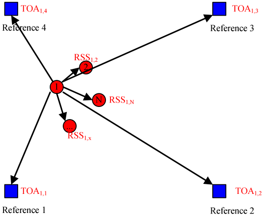
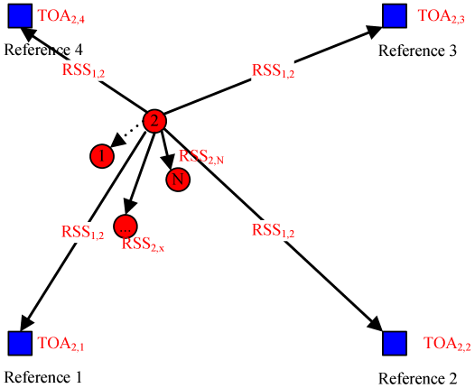
The proposed COTAR strategy engages the set of target nodes in a simple but effective cooperation to facilitate each other’s positioning. Consider the target nodes sending beacon packets one by one in a sequential manner. Due to the wireless broadcast advantage, when one target node transmits beacon signals, all the other target nodes in the vicinity can hear and measure the received-signal-strength from the transmitting node rather accurately. These RSS measurements contain valuable information about the relative distances and geological topology of the set of target nodes, which, when properly harnessed, can serve as useful calibration to compensate and mitigate localization errors.
To exploit all this neighboring RSS information, we propose the following COTAR localization strategy depicted in Figure 1:
(A)
(B)
The first target node starts out sending a beacon signal, and all the reference nodes measure and record the TOA of the beacon packet. At the same time, all the subsequent target nodes also measure the RSS from the transmitting target node.
Starting from the second target node, each target node will embed all the RSS it has measured from the previous target nodes in the payload of its beacon packet, and broadcasts. That is, the second target node transmits to all the reference nodes the RSS information between the first target node and itself; the third target node transmits the RSS information between the first target node and itself and between the second target node and itself; and so on. The reference nodes not only measure and record the TOA of these beacon packets, but also try to demodulate and decode the beacon packets to obtain the embedded RSS information.
Finally, the reference nodes share all the TOA information (between targets nodes and reference nodes) and all the RSS information (between target nodes) they have collected and perform centralized computation, either at one of the reference nodes or a dedicated control center. The centralized computation estimates the positions of all the target nodes in a single batch, and may implement different estimation methods, some of which are optimal and others suboptimal. In this paper, we consider formulating the problem as as a maximum likelihood position estimation problem, and further propose a linear simplification of the ML method to render a fast and efficient implementation through iterative refinement.
Here are a few comments:
(1) The proposed cooperative strategy is simple and practical, and incurs very minimal cooperative overhead. Compared to non-cooperative localization strategies where the target nodes must each send a beacon packet anyway, the additional requirement imposed by COTAR is for the target nodes to record and include in its beacon packet the RSS measurements. In practical systems, any (wireless) packets, including load-less beacon packets, must consist a sufficient packet-head to provide such information as where the packet is originated from. In many systems, there is also a minimal payload length required for a wireless packet, such that the packet does not become too short to easily slip off without being detected. As such, in which case the RSS information actually gets a free ride.
(2) The proposed strategy works for any set of target nodes that are in the vicinity of each other and willing to cooperate, but a practical question arises as what is a good value for . It is expected that the overall localization performance will improve with (with a diminishing return), but to engage many nodes in cooperation can be expensive or difficult in practical scenarios. Further, the communication overhead (recall that the th target node is expected to convey RSS measurements to the reference nodes) as well as the complexity of the centralized estimation also increase with . As we will show later in our analytical and simulation results, it is actually quite unnecessary to pull many nodes. Two to four cooperating nodes are sufficient, and in many cases, a mere engagement of two nodes () promises to delivery most of the cooperative gain.
(3) In the COTAR strategy, the reference nodes are expected to not only measure the TOA of beacon packets, but also extract from them the embedded RSS information. It is not necessary for all the reference nodes to correctly decode all the RSS information; as long as one out of the reference nodes gets it (and conveys it to the central node), an optimal joint estimation can proceed. In the rare case when none of the reference nodes succeeds in deducing a particular RSS information, the system may adopt one of the following two strategies. (i) First, the reference nodes can forward their individual reception of the beacon packets using, for example, amplify-and-forward (AF) or other ostensible signal-relaying technologies [15], to the central node for joint decoding. The central node is thus supplied with noisy copies of the beacon packet with a diversity order of at least , and has a considerably higher probability of extracting the RSS information than individual reference nodes can. (ii) Alternatively or as a last resort, the system can simply give up on the missing RSS information, and perform joint localization without having all the RSS information in place. Depending on how many and what RSS measurements are missing, the localization accuracy may be affected. We will discuss this issue in detail later, but in general, considering the rather small probability that none of the reference nodes has deduced the RSS information, the overall impact of missing RSS is very small.
IV Maximum Likelihood Position Estimation Using Joint TOA and RSS
Having discussed the general COTAR protocol, we now elaborate the maximum likelihood algorithm the central node performs to simultaneously estimate all the target positions through the collection of TOA and RSS information.
IV-A Path Loss among Target Nodes
Let be the horizontal and vertical coordinates of the actual positions for the targets nodes ( and are each dimensional column vectors). From the radio propagation attenuation model, we can write the average path loss between a pair of target nodes and , in the unit of dB, as:
| (6) |
where is the path-loss at the calibration distance, which is a constant and does not affect the localization accuracy.
The effect of multi-path, scattering, and shadowing phenomena may be collectively modeled as a multiplicative channel coefficient that follows a logarithmically Gaussian distribution. When expressing the channel attenuation in dB, the multiplicative coefficient becomes an addictive (noise) term that follows the Gaussian distribution (in dB). Since there are target nodes, the actual path loss between any pair of target nodes can be expressed in an dimensional column vector as
| (7) |
IV-B Time-Of-Arrival from Target Nodes to Reference Nodes
The distances between the th reference node and all the target nodes can be expressed using an dimensional column vector function:
| (8) |
The time of arrival (TOA) for the th target node’s signal arrives at all the reference nodes will ideally take the form as follows:
| (9) |
where is the speed of the waveform propagation, which is m/s for radio frequency signals. We arrange all TOAs from each target nodes to each reference nodes into one single dimensional TOA vector as
| (10) |
All this TOA estimation error is modeled as an dimensional Gaussian-distributed error vector . Hence, the noisy TOA vector from each target node to each reference node can be written as:
| (11) |
IV-C Path Loss between Target Nodes and Reference nodes
The average path loss between each target node and all reference nodes, in the unit of dB, as:
| (12) |
where is the path-loss at the calibration distance, which is a constant and does not affect the localization accuracy. We also rearrange all the RSS between each target node and each reference node in a single dimensional column vector as:
| (13) |
The effect of multi-path, scattering, and shadowing phenomena may be collectively modeled as a multiplicative channel coefficient that follows an addictive Gaussian noise term in logarithmical domain using unit dB. Since there are target nodes, the actual path loss between each target node and any reference node can be expressed in an dimensional column vector as
| (14) |
IV-D Unified RSS and TOA observation vector function
For a compact representation, we subsume the expected path-loss vector and all the expected TOAs in a single column vector consisting of rows, termed observation vector:
| (15) |
The true observation can be written as the sum of the observation vector and a Gaussian noise vector :
| (16) |
where the noise vector is given by
| (17) |
The observation error denotes the measurement distortion caused by various imperfect conditions regarding RSS and TOA, and is assumed to be a multivariate random vector with dimensional positive-definite covariance matrix:
| (18) |
IV-E Simplification through Taylor Expansion
The vector function , , and are nonlinear, which makes the measurement vector function technically challenging to handle. To make real-time computation possible, we approximate them using a single linear function by Taylor expanding them at the vector point . Mathematically, it can be written as follows:
| (19) |
where is the partial derivative matrix for each measurement on each unknown variable. The partial derivative matrix can be further written a dimensional matrix as follows:
| (24) |
whose elements and represent the partial derivatives of the th element in the observation vector with respect to the th target node’s horizontal coordinate and vertical coordinate respectively. is the dimension of the observation vector , and is the initial position vector.
IV-F Partial Derivative Matrix
A key computation step in the proposed joint estimation is the computation of the partial derivative matrix , which consists of two parts:
| (28) |
where the sub-matrices is the partial derivative matrix pertaining to the RSS measurements between any two target nodes, is the TOA measurements between target nodes and reference nodes), and is the RSS measurement between each target node and each reference node, respectively.
The sub-matrix has rows and columns, where rows correspond to pairs of target nodes, and columns correspond to the target nodes’ horizontal and vertical positions. The exact formulation of is defined as follows:
| (33) |
A row vector corresponds to the RSS between the th and th target nodes. It has four non-zero elements in the positions , , and , and is zero everywhere else:
| (35) |
The partial derivative matrix for TOA, , can be further decomposed to sub-matrices, each corresponding to the TOA derivative matrix for one target nodes with respect to its horizontal and vertical coordinates:
| (42) |
Each submatrix is an dimensional column matrix, denoting the partial derivatives of the TOA values, measured by the reference nodes about the th target node, with respect to the th target node’s horizontal coordinates:
| (43) |
Submatrices are similar, but the partial derivative is with respect to the the vertical coordinate pf the th target node:
| (44) |
Combining (8) and (9), and after simplification, the partial derivative sub-matrices can be written as follows:
| (49) |
| (54) |
where is the speed of light.
The partial derivative matrix for RSS between each target node and each reference node, , can be further decomposed to sub-matrices, each corresponding to the TOA derivative matrix for one target nodes with respect to its horizontal and vertical coordinates:
| (59) |
Each submatrix is an dimensional column matrix, denoting the partial derivatives of the RSS values, measured by the reference nodes about the th target node, with respect to the th target node’s horizontal coordinates:
| (60) |
Submatrices are similar, but the partial derivative is with respect to the the vertical coordinate pf the th target node:
| (61) |
IV-G Joint ML Estimation with Linear Approximation
Having computed the partial derivative matrix , we now discuss position estimation through maximum likelihood method and its efficient implementation.
Since the noise in the observation vector function is assumed Gaussian distributed, we can write the probability distribution function (pdf) at the vector point as:
| (71) |
where denotes the determinant of , the superscript denotes the matrix inverse, and is the dimension of .
The maximum likelihood estimator calculates the value that maximizes (71). Equivalently, it minimizes the quadratic term:
| (72) |
We further define
| (73) |
Minimizing is a reasonable criterion for determination of an estimator even when the measurement error cannot be assumed to be Gaussian distributed. In this case, the resulting estimator is called the least squares estimator and is regarded as a matrix of weighting coefficients. Therefore, we turn the position estimation problem to solving the equation of .
From its definition, is a symmetric matrix, i.e., . Since , it follows that , which shows that is a symmetric matrix. Therefore, we can obtain:
| (75) |
We assume that the matrix of is nonsingular. Thus the solution of (75) can be expressed as:
| (76) |
IV-H Iterative Estimation Refinement
Note that (77) suffers from the inaccuracy caused by approximating a nonlinear function using the linear Taylor expansion in (19) especially when are far away from the actually position . To mitigate the error and improve the estimation accuracy in (77), we propose to solve this problem through iterative refinement, in which the estimated position of the previous iteration is used as the initial position for the next refining iteration. To start, when we have no a priori knowledge, we may take the center point (or any point) of the scenario as the initial location for all the target nodes. For example, suppose reference nodes are placed in the corner of a square area with meters per side, the proposed iterative localization proceeds as follows:
| (78) |
where is the iteration index.
It is expected that a good choice for the initial position helps expedite the process while a bad one may delay the convergence, but this appears to be a non-issue, since our algorithm converges very fast. Through extensive simulations, we show that it generally takes no more than two to three iterations to arrive at an accurate estimation, even when the initial position is set very far from the actual position.
In the case of mobile tracking, when the previous-time position is used as the initial position to estimate the next-time position, a single iteration suffices. The iterative process not only improves the localization accuracy, but also makes the strategy particularly suitable for mobile localization. When target nodes are moving and their continuous trace needs to be detected, it is very natural to use their previous locations as the starting point to estimate the next locations. Unless the nodes are moving at extremely fast speeds, the new locations will not be far from the old ones, and hence a single iteration suffices, allowing efficient position tracking.
V Analysis of Estimation Accuracy and performance comparisons
To provide a theoretical support, we first evaluate the Cramer-Rao lower bound for the proposed cooperative TOA-RSS localization scheme. We next analyze the theoretical root mean square error of the proposed maximum likelihood position estimation algorithm. We compare the bounds of the proposed localization scheme with the existing localization schemes.
V-A Cramer Rao lower bounds (CRB) analysis
The CRB of an unbiased estimator is given by
where is the Fisher information matrix (FIM) given by [17]:
| (81) |
where is the logarithm of the joint conditional probability density function. We can further write
| (82) |
The CRB on the standard derivation of each target node’s position estimation is:
| (83) |
The expression of is different for each localization estimation scheme.
Existing Localization Schemes
The traditional RSS scheme [18][19] uses only the RSS from a sensor node to all the reference nodes ( RSS measures per sensor) to perform position estimation. We have:
| (84) |
where .
Similarly, for the traditional TOA scheme [18][19], only the TOA at the reference nodes TOA measures per sensor is used for estimation. The logarithm of the joint conditional probability density function can be written as:
| (85) |
where , and .
The existing non-cooperative hybrid TOA-RSS schemes exploit both the RSS and TOA from each senor to all the reference nodes (, which exploits total modality measures per sensor, including modality measures per sensor for TOA and another modality measures per sensor for TOA). As discussed in [17], for the hybrid TOA-RSS scheme, it is given by
| (86) |
We further substitute (84)(85)(V-A) into (V-A)(V-A) respectively, and after some rather involved numerical calculation, we obtain the CRB for traditional RSS, TOA, and hybrid TOA-RSS localization schemes.
The Proposed New Scheme
The new cooperative TOA-RSS scheme developed here makes use of not only the TOA from each sensor to all the reference nodes but also the RSS between the two neighboring sensors, to jointly estimate the poses of both sensors ( modality measures for sensors). We can write the logarithm of the joint conditional probability density function as follows:
| (87) |
where .
Similar to the procedure of calculation traditional localization schemes, substituting (87) in (V-A) and (V-A) and after simplification, we can compute the Cramer-Rao bound for the proposed new scheme.
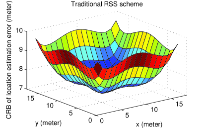
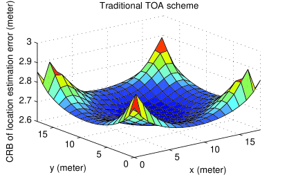
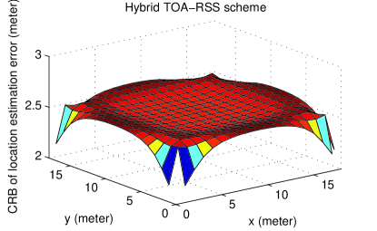
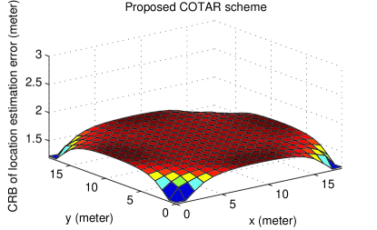
The Cramer-Rao bounds for different schemes are shown in Fig.2, where 4 reference nodes are deployed at the four corners of an meters’ square scenario in clear line-of-sight situation. Four cooperative target nodes help each other in the proposed COTAR scheme at the four corners of a meters’ square. It is clear to see that the RSS only scheme has a poor localization accuracy from 8 to 10 meters. The traditional TOA scheme obtains a better accuracy of 2.7 meters in the middle and 2.9 meters at the four corners. The hybrid TOA-RSS scheme helps improve the accuracy of traditional TOA scheme at the four corners to 2.2 meters, but not in the middle of the scenario. The proposed scheme has an excellent localization accuracy, which achieves 1.55 meters’ accuracy in the middle and 1.2 meters’ accuracy at the four corners of the scenario.
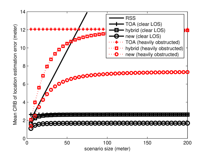
We further invest the localization accuracy vs increase of scenarios size for different localization schemes in different channel conditions in Fig.3. It is shown that the RSS scheme’s localization error increases linearly fast, which makes it useless in a large scenario. On the contrary, the accuracy of traditional TOA scheme does change with the increase of range. The hybrid TOA-RSS scheme can only improve the accuracy when the scenario size is less than 10 meters’ in clear line-of-sight situation, and 100 meters in heavily obstructed situation. Otherwise, it can only obtains the same performance as traditional TOA scheme. For the proposed COTAR scheme, it performs excellently in any scenario size. It cuts half down the localization error from to meters in heavily obstructed scenario, and improves the accuracy from meters to meters in clear line-of-sight situation.
V-B Root Mean Square Error Analysis for ML Estimation
We now analyze the performance error of the proposed detector in (77), and evaluate the errors with respect to different positions .
The expression in (77) shows that when the measurement vector is Gaussian distributed, the estimation vector becomes a dimensional Gaussian random vector with a pdf:
| (88) |
where , the covariance matrix of the estimation vector , is defined as:
| (89) |
There are two types of inaccuracy associated with a Gaussian distributed variable, the mean bias and the variance . The estimation error should in general consist of both:
| (90) |
On the other hand, substituting (16) into (77) and rearranging terms, we can write the estimation vector as:
| (91) |
It is clear from (91) that the estimation error comprises both a linearizing error and a noise term. The linearizing error in (91) contributes to the mean bias:
| (92) |
The estimator will be unbiased, if is a linear vector function; but since it is not, the inaccuracy of the Taylor expansion in (19) thus introduces non-zero mean bias to the estimation. From (19), we also know that if the initial position is sufficiently close to the actual position and , the linearizing error in (92) will become vanishingly small and can be safely ignored.
The residual noise in the estimation, caused by the measurement error vector , results in variation in the estimation results. This noise part is expressed as:
| (93) |
Here the error vector subsumes all the error contributors, including the measurement distortion of the signal TOA and the RSS between the two cooperative nodes, and others uncertainties in the system. It is reasonable to assume that the measurement distortion for TOA and RSS are unbiased, such that is a dimensional column vector following a zero-mean (vector) Gaussian distribution.
Since the mean bias is a constant vector given the initial position , the calculation for the covariance matrix of the estimation error is only affected by (93):
| (94) |
Note that the diagonal elements of denote the variances of the errors in the estimated positions.
Since the measurement distortion is Gaussian distributed with zero mean, the maximum likelihood or the least square estimator for the linearized model is the same as the minimum variance unbiased estimator. A scalar measure of the estimator accuracy is the root mean square error , which is defined as
| (95) |
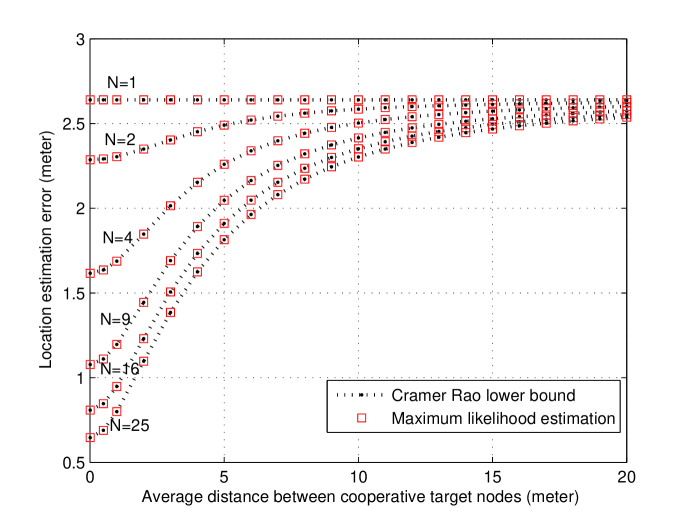
The RMS error bound of the proposed ML estimator for the COTAR scheme is plotted in Fig4 as a function of the distance between target nodes and the number of cooperative target nodes. For comparison, we also shown the CRB of the COTAR scheme in the same picture. We consider four reference nodes are deployed at the four corners of a meters’ square scenario, and target nodes are placed in a meters’ grid. The grid size is the distance between two closest cooperative target nodes. It is well-known that the CRB sets the lower bound of a scheme for all the possible detectors, and may be achieved by an unbiased optimal detector. That our root mean square error bounds matches perfectly with the CRB (shown in Fig. 4), and that our simplified iterative algorithm practically achieves these bounds (as will be shown in simulations), clearly indicates the efficiency of the proposed detection algorithm. We also find that the gird size and the number cooperative target nodes are two important factors to the localization accuracy. For example, increasing the number of cooperating nodes from 1 (non-cooperative) to 25 can effectively improve the localization accuracy from 2.7 meters to 0.7 meters. It also shows that the cooperative target nodes should not be too far away. Due to the quickly-decreasing accuracy of RSS with distance, a close neighbor can do more to improve localization accuracy than several remote collaborators.
VI Simulation results
VI-A COTAR vs Existing Strategies
We now conduct computer simulations to study the realistic performance for the proposed COTAR localization algorithm. We firstly consider four reference nodes () are located at the four corners of a square area with edge length meters.
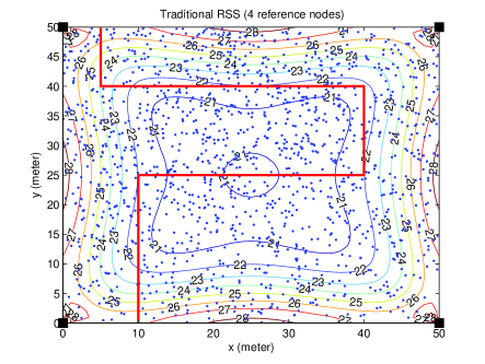
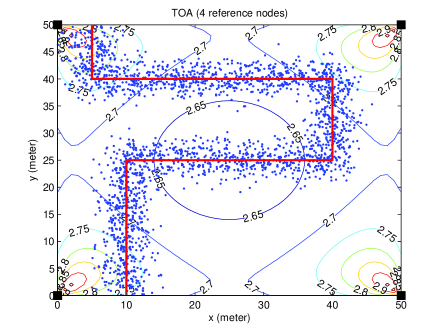
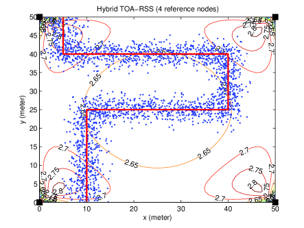
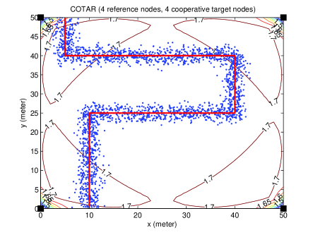
To start, we consider four cooperating target nodes that move together in the square area and always stay at the four corners of a meter’s grid. Four localization strategies based on RSS, TOA, hybrid TOA-RSS, and the proposed COTAR, are evaluated:
-
1.
RSS-only: Each target node sends a beacon packet independently, and all the reference nodes measure the RSS information, and route them to a central node for maximum likelihood estimation. The target nodes do not cooperate, and RSS measures are used to estimate the position of any one target node.
-
2.
TOA-only: It is similar to RSS-only, but the reference nodes measure the TOA information instead. TOA measures are used to estimate the position of any one target node.
-
3.
Hybrid TOA/RSS 333For convenience, we call the RSS between target nodes and reference nodes “remote-RSS” and the RSS between two (nearby) target nodes “neighboring-RSS.” [9][10]: It is similar to RSS-only and TOA-only, but the reference nodes measure both the TOA and the RSS information. The scheme is again non-cooperative, and measures ( TOA and RSS) are used to estimate the position of any one target node.
-
4.
COTAR: As discussed before, the scheme is one that combines TOA and neighboring-RSS. A set of target nodes are engaged in a simple cooperation, and TOA measures, neighboring-RSS measure, and remote RSS information are used to jointly estimate the positions of the target nodes. In the simulation, the scenario center with coordinates is always used as the initial position for both target nodes, and two iterations are used in the iterative refinement.
The localization results for tracking mobile nodes are shown in Fig.5, where red zigzag line shows the moving track of a group of four cooperative target nodes, and blue dots represents the estimated positions of different schemes. The results of 15 experiments are shown444We performed more experiments, but they make the picture too dense to see., and in each experiment, position tracking is performed in a continuous manner, with the previous estimated location serving as the starting point for the next one, and two iterations to estimate the incremental errors. Also shown in the figure are the performance contour. Because of the large distance between each target nodes and the reference nodes, we are not surprised to see that the RSS-only method performs rather poorly, with the estimated positions scatter all over the place, yielding an estimation error RMS of as large as to meters. In comparison, the traditional TOA-only method is much less sensitive to the distance. It attains a satisfactory performance of 2.7 meters of error. When TOA and remote-RSS are combined as hybrid TOA-RSS scheme [9], only the performance of the four corners of the scenario is effectively improved(, where reference nodes are deployed), but not the most of other positions especially in the middle of the scenario. The proposed COTAR strategy provides a much better solution by leveraging both the good accuracy of the RSS between two neighboring target nodes in short distance and the large localization range from TOA techniques. COTAR achieves a high localization accuracy of less than 1.5 meter’s of distortion in the middle of the scenario, and 1.2 meters’ accuracy at the four corners.
VI-B Impact of Initial Position and Number of Iterations
We next study the impact of the number of iterations and the initial position on the localization accuracy. The same meters’ square area with reference nodes and cooperating target nodes is simulated. We consider the clear line-of-sight channel situation, the cooperative grid size to be 1 meter, and use the scenario center as the initial position for the target nodes.
We evaluate the gap between the actual localization error and the theoretical lower bound. This gap is plotted in Figure 6(A) and Figure 6(B) for one and two estimation iterations, respectively. We see that the accuracy of the starting point can make a difference, but only to the first iteration. As shown in Figure 6(A), with only one iteration, the localization strategy may achieve a tiny RMS error of meter from the lower bound near the grid center, but an accuracy gap of as large as 1.9 meters near the four edges. It is interesting to observe that, when the target nodes get very close to the corner points, their closeness to one of the reference nodes, and hence the accurate TOA measures, can help mitigate the negative impact caused by the inaccurate starting point (and the insufficient iterations). As the iterations increases to two, the accuracy gap quickly drops to near-zero across the entire region. In the simulated (meter) grid, it appears that when the initial position is not offset by more than 10 meters from the actual target locations, one iteration is enough; Otherwise, two iterations suffice to bring down the estimation error to the lower bound.
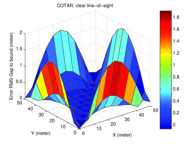
(A)
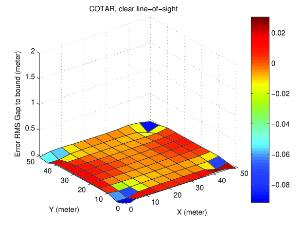
(B)
VI-C Impact of Number of Reference Nodes and Cooperative Nodes
We first consider there are more than 4 reference nodes, say 9 reference nodes in the scenario. The 9 reference nodes are evenly deploy at every 25 meters as black in Fig.7. We study the performance of the hybrid TOA-RSS scheme and the proposed COTAR scheme and plot the simulation results in Fig.7. From this figure, we see that the ML estimation algorithm works robustly in any position in the scenario, and increasing reference nodes number from 4 to 9 can effectively improve the localization accuracy for both hybrid TOA/RSS and COTAR schemes. At the middle of the scenario, the localization accuracy improve from 2.65 to 1.65 meters for hybrid TOA-RSS, and 1.7 to 1.05 meters for COTAR.
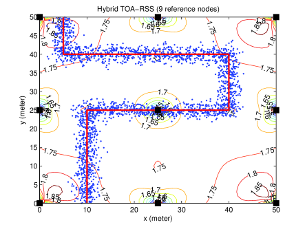
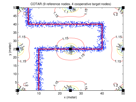
We further study the localization performance with more than 4 cooperative nodes. The same system set up is used, and we consider the cases when cooperative target nodes are available for cooperation.
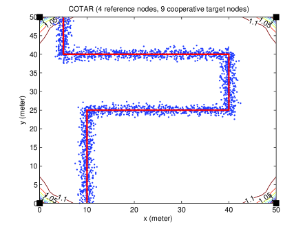
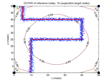
The simulation results, plotted in Figure 8, clearly speaks for the importance of increasing number of cooperative nodes. With the help of 9 cooperating target nodes, COTAR can achieves 1.05 meters’ accuracy in most of the area. If we further increase the number of cooperative nodes to 16, we are glad to find that COTAR obtains an excellent cooperative localization performance of only meters’ error.
VI-D Impact of Missing RSS
As mentioned before, although uncommon, it is possible for some RSS information to miss in the equation, either because a target node fails to estimate it in the first place, or because all the reference nodes fail to decode it from the beacon packet. In such cases, the joint estimation should proceed without this information. One possible way to handle such abnormality is to reformat all the relevant matrices in (33) by extracting the corresponding row(s) from (35). A more convenient way is to simply set the missing RSS information to be zero in the original formulation in (35) without changing the dimension of the partial derivative matrix.
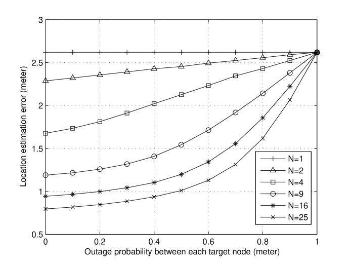
The potential impact of missing RSS information on the COTAR performance is presented in Figure 9. Cases with different cooperating nodes having different probability (percentage) of missing RSS are evaluated. It is encouraging to see that the localization accuracy degrades rather gracefully with missing RSS. When the missing RSS is below 20 percentage, the increase in average RMS error is very minor – no more than 0.07 meters for cooperating nodes and negligible for cooperating nodes. When all the RSS is missing (100% missing probability), the COTAR strategy reduces to the non-cooperative TOA-only scheme with RMS error of about 2.67 meters. It is also evident from the simulation that increasing the number of cooperating nodes is an effective way to compensate RSS loss and reduce localization error.
VI-E Tracking Highly Mobile Nodes
The proposed localization strategy is also evaluated in a highly mobile system such as the 3G mobile cellular phone networks. We consider four base stations situated at the four corners of a square grid with edge length meters, acting as the reference nodes (). Suppose a pair of cell phones are moving together in the grid with a high speed of up to 160 km/hour. Suppose the cell phones move with random directions and when they hit the boundary, they bounce off like the reflection of a ray of light. The COTAR algorithm is used to track the mobile positions of these cell phones, where the previous estimate is used as the starting point for the next estimate, and either one or two iterations of refinement is performed. To make the system simple and light-load, we consider a very low sample rate, such that beacon packets are transmitted and localization is performed once every 5 seconds.
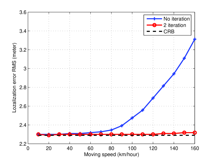
The localization RMS error is plotted at a function of the mobile speed in Figure 10. We can see that when the nodes move at a slow to medium speed ( km/hour), 1 iteration is enough to obtain good accuracy. As the mobile peed increases beyond 80 km/hour, since our sample rate is rather low and two succeeding sampling points are fairly separated, and since the localization errors may accumulate, 1 iteration becomes a little insufficient, resulting an increase of localization RMS error from 2.55 meters (at 80 km/hour) to 3.60 meters (at 160 km/hour). To bring down the error, one can simply add one more iteration, such that the localization error is kept consistently low and close to the lower bound.
VII Conclusion
Low-cost and accurate wireless localization is challenging, due to the limited bandwidth, hardware and computational resources, as well as possibly severe multi-path fading and non-LOS conditions. In the paper, we propose an effective cooperative-TOA-and-RSS localization strategy which is simple, practical, and inexpensive to deploy, and which requires no additional hardware than the usual cheap sensors (like Zigbee nodes). By engaging two or more target nodes in simple but effective cooperation, and by leveraging useful estimation and detection techniques, the new COTAR strategy reaps the merits of both TOA (i.e. decent performance fora a large localization range) and RSS (i.e. high accuracy in short distances), without incurring much cooperation overhead to the target nodes. Analytical and simulation results confirm the good performance of the new strategy in both clear and heavily obstructed cases. The proposed COTAR strategy is particularly useful for (high-speed) mobile localization, since the algorithm can naturally and efficiently achieve incremental update through iterative refinement.
References
- [1] A. Boukerche, H. A. B. Oliveira, E. F. Nakamura, and A. A. F. Loureiro, “Localization systems for wireless sensor networks,” IEEE Transaction on Wireless Communications, vol. 14, pp. 6-12, Dec. 2007
- [2] L. Jetto, S. Longhi, and G. Venturini, “Development and experimental validation of an adaptive extended Kalman filter for the localization of mobile robots,” IEEE Trans. Robotics and Automation, 1999.
- [3] A. Varshavsky, M. Y. Chen, E. de Lara, J. Froehlich, D. Haehnel, J. Hightower, A. LaMarca, F. Potter, T. Sohn, K. Tang, and I. Smith, “Are GSM phones THE solution for localization?” Proc. IEEE Workshop on Mobile Computing, 2006.
- [4] A. P. Lserte, A. I. Perez-Neira, and M. A. L. Hernandez, “Iterative algorithm for the estimation of distributed sources localization parameters”, Proceedings of the 11th IEEE Signal Processing Workshop on Statistical Signal Processing, Aug 6-8. 2001 pp.528-531.
- [5] S. Thrun, D. Fox, W. Burgard, and F. Dellaert, “Robust Monte Carlo localization for mobile robots,” Artificial Intelligence, 2001
- [6] M. L. Sichitiu and V. Ramadurai, “Localization of wireless sensor networks with a mobile beacon,” Proc. of IEEE Intl. Conf. Mobile Ad-hoc and Sensor Sys., 2004.
- [7] E. Elnahrawy, X. Li, and R. P. Martin, “The limits of localization using signal strength: A comparative study,” Proc IEEE SECON, 2004.
- [8] N. B. Priyantha, H. Balakrishnan, E. D. Demaine, and S. Teller, “Mobile-assisted localization in wireless sensor networks,” Proc. of IEEE Infocom, 2005.
- [9] K. C. Ho, and S. Ming, “Passive source localization using time differences of arrival and gain ratios of arrival”, IEEE Transactions on signal processing, Vol. 56, Issue 2, pp. 464-477, Feb. 2008.
- [10] L. Cong and W. Zhuang, “Hybrid TDOA/AOA mobile user location for wideband CDMA cellular systems,” IEEE Trans. Wireless Commun., vol. 1, pp. 439-447, Jul. 2002.
- [11] N. Patwari, J. N. Ash, S. Kyperountas, A. O. Hero III, R. L. Moses, and N. S. Correal, “Locating the nodes: Cooperative localization in wireless sensor networks,” IEEE Signal Processing Magazine, pp. 54-69, July, 2005
- [12] Y. Qi, Wireless geolocation in a non-line-of-sight environment, Ph.D. Dissertation, Princeton University, Dec. 2004.
- [13] S. Kim, H.L. Bertoni, and M. Stern, “Pulse propagation characteristics at 2.4GHz inside buildings,” IEEE Transactions on Vehicular Technology, 45(3):579-592, August 1996.
- [14] M. S. Wilcox, Techniques for Predicting the Performance of Time-of-Flight based local positioning Systems, Ph.D. Dissertation, University of London, Sept, 2005.
- [15] X. Bao, and J. Li, “Efficient Message Relaying for Wireless User Cooperation: Decode-Amplify-Forward (DAF) and Hybrid DAF and Coded-Cooperation”, IEEE transaction on wireless Communications, Vol. 6, No. 11, Nov. 2007.
- [16] Z. Sahinoglu and A. Catovic, “A hybrid location estimation scheme (H-LES) for partially synchronized wireless sensor networks,” in IEEE 2004 Int. Conf. Communications Conf. Rec., Paris, France, June 2004, pp. 3797 C3801.
- [17] A. Catovic, and Z. Sahinoglu, “The Cramer-Rao bounds of hybrid TOA/RSS and TDOA/RSS location estimation schemes”, IEEE Communication Letters, VOL. 8, NO. 10, OCT 2004.
- [18] K. Pahlavan, X. Li, and J. P. Makela, “Indoor geolocation science and technology,” IEEE Commun. Mag., vol. 40, no.2, pp.112-118, Feb. 2002.
- [19] N. Patwari, O. A. Hero, III , M. Perkins, N.S. Correal, and R.J. O’Dea, “Relative location estimation in wireless sensor networks,” IEEE Trans. Signal Processing, vol. 51, pp. 2137-2148, Aug. 2003.