Zone diagrams in compact subsets of uniformly convex normed spaces

Abstract.

A zone diagram is a relatively new concept which has emerged in computational geometry and is related to Voronoi diagrams. Formally, it is a fixed point of a certain mapping, and neither its uniqueness nor its existence are obvious in advance. It has been studied by several authors, starting with T. Asano, J. Matoušek and T. Tokuyama, who considered the Euclidean plane with singleton sites, and proved the existence and uniqueness of zone diagrams there. In the present paper we prove the existence of zone diagrams with respect to finitely many pairwise disjoint compact sites contained in a compact and convex subset of a uniformly convex normed space, provided that either the sites or the convex subset satisfy a certain mild condition. The proof is based on the Schauder fixed point theorem, the Curtis-Schori theorem regarding the Hilbert cube, and on recent results concerning the characterization of Voronoi cells as a collection of line segments and their geometric stability with respect to small changes of the corresponding sites. Along the way we obtain the continuity of the Dom mapping as well as interesting and apparently new properties of Voronoi cells.

1. Introduction

A zone diagram is a relatively new concept related to geometry and fixed point theory. In order to understand it better, consider first the more familiar concept of a Voronoi diagram. In a Voronoi diagram we start with a set $X$, a distance function $d$, and a collection of subsets $(P_{k})_{k\in K}$ in $X$ (called the sites or the generators), and with each site $P_{k}$ we associate the Voronoi cell $R_{k}$, that is, the set of all $x\in X$ the distance of which to $P_{k}$ is not greater than its distance to the union of the other sites $P_{j}$, $j\neq k$. On the other hand, in a zone diagram we associate with each site $P_{k}$ the set $R_{k}$ of all $x\in X$ the distance of which to $P_{k}$ is not greater than its distance to the union of the other sets $R_{j}$, $j\neq k$. Figures 2 and 2 show the Voronoi and zone diagrams, respectively, corresponding to the same ten singleton sites in the Euclidean plane.

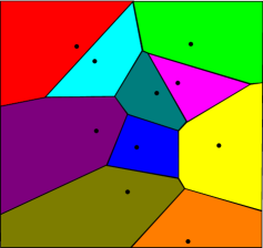
Figure 1. A Voronoi diagram of 10 point sites in a square in $(\mathbb{R}^{2},\ell_{2})$.

Figure 2. A zone diagram of the same 10 points as in Figure 2.

At first sight, it seems that the definition of a zone diagram is circular, because the definition of each $R_{k}$ depends on $R_{k}$ itself via the definition of the other cells $R_{j}$, $j\neq k$. On second thought, we see that, in fact, a zone diagram is defined to be a fixed point of a certain mapping (called the Dom mapping), that is, a solution of a certain equation. While the Voronoi diagram is explicitly defined, so its existence (and uniqueness) are obvious, neither the existence nor the uniqueness of a zone diagram are obvious in advance. As a result, in addition to the problem of finding algorithms for computing zone diagrams, we are faced with the more fundamental problem of establishing their existence (and uniqueness) in various settings, and with the problem of reaching a better understanding of this concept.

The concept of a zone diagram was first defined and studied by T. Asano, J. Matoušek and T. Tokuyama [2, 3] (see also [4]), in the case where $(X,d)$ was the Euclidean plane, each site $P_{k}$ was a single point, and all these (finitely many) points were different. They proved the existence and uniqueness of a zone diagram in this case, and also suggested a natural iterative algorithm for approximating it. Their proofs rely heavily on the above setting. Several other papers related to zone diagrams in the plane have been published, e.g., those of T. Asano and D. Kirkpatrick [1], of J. Chun, Y. Okada and T. Tokuyama [6], and recently of S. C. de Biasi, B. Kalantari and I. Kalantari [9].

Shortly after [3], the authors of [22] considered general sites in abstract spaces, called $m$-spaces, in which $X$ is an arbitrary nonempty set and the “distance” function should only satisfy the condition $d(x,x)\leq d(x,y)\,\,\,\,\forall x,y\in X$ and can take any value in the interval $[-\infty,\infty]$. They introduced the concept of a double zone diagram, and using it and the Knaster-Tarski fixed point theorem, proved the existence of a zone diagram with respect to any two sites in $X$. They also showed that in general the zone diagram is not unique. In a recent work by K. Imai, A. Kawamura, J. Matoušek, Y. Muramatsu and T. Tokuyama [14], the existence and uniqueness of the zone diagram with respect to any number of general positively separated sites in the $n$-dimensional Euclidean space $\mathbb{R}^{n}$ was announced. The proof is based on results from [22] and on an elegant geometric argument specific to Euclidean spaces. Very recently some of these authors have generalized this result to finite dimensional normed spaces which are both strictly convex and smooth [15].

In the present paper we prove the existence of zone diagrams with respect to finitely many pairwise disjoint compact sites contained in a compact and convex subset of a (possibly infinite dimensional) uniformly convex space, provided that either the sites or the convex subset satisfy a certain mild condition. This mild condition holds, for instance, if either the convex subset $X$ has a strictly convex boundary or the sites are contained in the interior of $X$ relative to the affine hull spanned by $X$ (and $X$ is arbitrary). The proof is based on the Schauder fixed point theorem, the Curtis-Schori theorem regarding the Hilbert cube, and on recent results concerning the characterization of Voronoi cells as a collection of line segments and their geometric stability with respect to small changes of the corresponding sites (see Sections 3 and 4). Along the way we obtain the continuity of the Dom mapping (Proposition 6.1) in a general setting and interesting properties of Voronoi cells, namely Lemma 5.1 and Lemma 5.2. Although Voronoi diagrams have been the subject of extensive research during the last decades [5, 18, 12], this research has been mainly focused on Euclidean finite dimensional spaces (in many cases just $\mathbb{R}^{2}$ or $\mathbb{R}^{3}$), and it seems that these lemmata are new even for $\mathbb{R}^{2}$ with a non-Euclidean norm.

It may be of interest to compare our main existence result with the recent existence result described in [15]. On the one hand, our result is weaker than that result, since we only prove the existence of a zone diagram in a compact and convex set, while in [15] uniqueness is also proved and the setting is the whole space $\mathbb{R}^{n}$. In addition, it seems that some of the arguments in [15], although only formulated for finitely many compact sites, can be extended to infinitely many, positively separated closed sites. On the other hand, our result is stronger in the sense that we allow infinite dimensional spaces and we do not require the smoothness of the norm. As a matter of fact, the counterexamples mentioned in [15] show that uniqueness does not necessarily hold if the norm is not smooth. In any case, the strategies used for proving these two results are completely different: in [15] the authors use the existence of double zone diagrams (based on the Knaster-Tarski fixed point theorem) and several geometric arguments, and here we use the Schauder fixed point theorem, the Curtis-Schori theorem regarding the Hilbert cube, and several general results about Voronoi cells in uniformly convex normed spaces and elsewhere.

The structure of the paper is as follows: in Section 2 we present the basic definitions and notation. In Section 3 we provide the outline of the proof of the main result. In Section 4 we formulate several claims which are needed in the proof. The proof itself is given in Sections 5, 6 and 7. We conclude the paper with Section 8, which contains open problems and two pictures of zone diagrams.

We note that although the setting in the main result is a compact and convex subset of a uniformly convex normed space, many of the auxiliary results actually hold in a more general setting with essentially the same proofs, and therefore we formulate and prove them there.

2. Definitions and Notation

In this section we present our notation and basic definitions. We consider a closed and convex set $X\neq\emptyset$ in some normed space $(\widetilde{X},|\cdot|)$, real or complex, finite or infinite dimensional. The induced metric is $d(x,y)=|x-y|$. We assume that $X$ is not a singleton, for otherwise everything is trivial.

The notation $|\theta|=1$ will always mean a unit vector $\theta$. Given $p\in X$ we set $\Theta_{p}=\{\theta:|\theta|=1,p+t\theta\in X\,\,\textnormal{for some}\,\,t>0\}$. This is the set of all directions such that rays emanating from $p$ in these directions intersect $X$ not only at $p$. We denote by $[p,x]$ the closed line segment connecting $p$ and $x$, i.e., the set $\{p+t(x-p):t\in[0,1]\}$. We denote by $B(x,r)$ the open ball of center $x$ and radius $r$. The notation $Y\approx Z$ means that the topological spaces $Y$ and $Z$ are homeomorphic.

Definition 2.1.

Given two nonempty sets $P,A\subseteq X$, the dominance region $\textnormal{dom}(P,A)$ of $P$ with respect to $A$ is the set of all $x\in X$ the distance of which to $P$ is not greater than its distance to $A$, that is,

$$\textnormal{dom}(P,A)=\{x\in X:d(x,P)\leq d(x,A)\}.$$

Here $d(x,A)=\inf\{d(x,a):a\in A\}$.

Definition 2.2.

Let $K$ be a set of at least 2 elements (indices), possibly infinite. Given a tuple $(P_{k})_{k\in K}$ of nonempty subsets $P_{k}\subseteq X$, called the generators or the sites, the Voronoi diagram induced by this tuple is the tuple $(R_{k})_{k\in K}$ of nonempty subsets $R_{k}\subseteq X$, such that for all $k\in K$,

$$R_{k}=\textnormal{dom}(P_{k},{\underset{j\neq k}{\bigcup}P_{j}})=\{x\in X:d(x,P_{k})\leq d(x,P_{j})\,\,\forall j\neq k,\,j\in K\}.$$

In other words, each $R_{k}$, called a Voronoi cell, is the set of all $x\in X$ the distance of which to $P_{k}$ is not greater than its distance to the union of the other $P_{j}$, $j\neq k$.

Definition 2.3.

Let $(X,d)$ be a metric space and let $K$ be a set of at least 2 elements (indices), possibly infinite. Given a tuple $(P_{k})_{k\in K}$ of nonempty subsets $P_{k}\subseteq X$, a zone diagram with respect to that tuple is a tuple $R=(R_{k})_{k\in K}$ of nonempty subsets $R_{k}\subseteq X$ such that

$$R_{k}=\textnormal{dom}(P_{k},\textstyle{\underset{j\neq k}{\bigcup}R_{j}})\quad\forall k\in K.$$

In other words, if we define $X_{k}=\{C:P_{k}\subseteq C\subseteq X\}$, then a zone diagram is a fixed point of the mapping $\textnormal{Dom}:\underset{{k\in K}}{\prod}X_{k}\to\underset{{k\in K}}{\prod}X_{k}$, defined by

(1) $$\textnormal{Dom}(R)=(\textnormal{dom}(P_{k},\textstyle{\underset{j\neq k}{\bigcup}R_{j}}))_{k\in K}.$$

For example, let $P_{1}=\{p_{1}\}$ and $P_{2}=\{p_{2}\}$ be two different sets in the Euclidean plane, or more generally, in a Hilbert space $X$. In this case the corresponding Voronoi diagram consists of two half-spaces: $\textnormal{dom}(P_{1},P_{2})$ is the half-space containing $P_{1}$ and determined by the hyperplane passing through the middle of the line segment $[p_{1},p_{2}]$ and perpendicular to it, and $\textnormal{dom}(P_{2},P_{1})$ is the other half-space. The zone diagram of $(P_{1},P_{2})$ exists by the results of [3] (in the case of the Euclidean plane), or [22] (in the general case), but it is not clear how to describe the zone diagram explicitly.

We now recall the definition of strictly and uniformly convex spaces.

Definition 2.4.

A normed space $(\widetilde{X},|\cdot|)$ is said to be strictly convex if for all $x,y\in\widetilde{X}$ satisfying $|x|=|y|=1$ and $x\neq y$, the inequality $|(x+y)/2|<1$ holds. $(\widetilde{X},|\cdot|)$ is said to be uniformly convex if for any $\epsilon\in(0,2]$, there exists $\delta\in(0,1]$ such that for all $x,y\in\widetilde{X}$, if $|x|=|y|=1$ and $|x-y|\geq\epsilon$, then $|(x+y)/2|\leq 1-\delta$.

Roughly speaking, if the space is uniformly convex, then for any $\epsilon>0$, there exists a uniform positive lower bound on how deep the midpoint between any two unit vectors must penetrate the unit ball, assuming the distance between them is at least $\epsilon$. In general normed spaces the penetration is not necessarily positive, since the unit ball may contain line segments. The plane $\mathbb{R}^{2}$ endowed with the max norm $|\cdot|_{\infty}$ is a typical example of this. A uniformly convex space is always strictly convex, and if it is also finite dimensional, then the converse is true too. The $n$-dimensional Euclidean space $\mathbb{R}^{n}$, or more generally, inner product spaces, the sequence spaces $\ell_{p}$, the Lebesgue spaces $L_{p}(\Omega)$, $p\in(1,\infty)$, and a uniformly convex product of a finite number of uniformly convex spaces, are all examples of uniformly convex spaces. See [7] and, for instance, [16] and [11] for more information regarding uniformly convex spaces.

We now recall three definitions of a topological character.

Definition 2.5.

The Hilbert cube $I^{\infty}$ is the set $I^{\infty}=\prod_{n=1}^{\infty}[0,1/n]$ as a topological space the topology of which is induced by the $\ell_{2}$ norm, or, equivalently, by the product topology.

Definition 2.6.

A topological space $X$ is said to be locally (path) connected if for any $x\in X$ and any open set $U$ containing $x$, there exists a (path) connected open set $V\subseteq U$ such that $x\in V$. $X$ is said to be weakly locally (path) connected, or (path) connected im kleinen, if for any $x\in X$ and any open set $U$ containing $x$, there exists a (path) connected set $C\subseteq U$ and an open set $V\subseteq C$ such that $x\in V$.

Definition 2.7.

Let $(X,d)$ be a metric space. Given two nonempty sets $A_{1},A_{2}\subseteq X$, the Hausdorff distance between them is defined by

$$D(A_{1},A_{2})=\max\{\sup_{a_{1}\in A_{1}}d(a_{1},A_{2}),\sup_{a_{2}\in A_{2}}d(a_{2},A_{1})\}.$$

Recall that the Hausdorff distance is different from the usual distance between two sets which is defined by

$$d(A_{1},A_{2})=\inf\{d(a_{1},a_{2}):a_{1}\in A_{1},a_{2}\in A_{2}\}.$$

Recall also that if $(X,d)$ is compact and we consider the set of all its nonempty closed subsets, then this space is a compact metric space with the Hausdorff distance as its metric [13].

We end this section with a definition which is pertinent to the formulation of our main result and some of our auxiliary assertions. It is followed by a brief discussion.

Definition 2.8.

Let $X$ be a closed and convex subset of a normed space. Let $p\in X$. Let $\theta\in\Theta_{p}$. Let $L(\theta)\in(0,\infty]$ be the length of the line segment generated from the intersection of $X$ and the ray emanating from $p$ in the direction of $\theta$. The point $p$ is said to have the emanation property (or to satisfy the emanation condition) in the direction of $\theta$ if for each $\epsilon>0$ there exists $\beta>0$ such that for any $\phi\in\Theta_{p}$, if $|\phi-\theta|<\beta$, then the intersection of $X$ and the ray emanating from $p$ in the direction of $\phi$ is a line segment of length at least $L(\theta)-\epsilon$. In other words, $L(\phi)\geq L(\theta)-\epsilon$. The point $p$ is said to have the emanation property if it has the emanation property in the direction of every $\theta\in\Theta_{p}$. A subset $C$ of $X$ is said to have the emanation property if each $p\in C$ has the emanation property.

The following examples illustrate the emanation property. In the first four the emanation property holds, and in the last one it does not hold.

Example 2.9.

$X$ is any bounded closed convex set and $p\in X$ is an arbitrary point in the interior of $X$ relative to the affine hull spanned by $X$.

Example 2.10.

The boundary of the bounded closed and convex $X$ is strictly convex (if $a\neq b$ are two points in the boundary, then the open line segment $(a,b)$ is contained in the interior of $X$ relative to the affine hull spanned by $X$) and $p\in X$ is arbitrary. Any ball in a strictly convex space has a strictly convex boundary.

Example 2.11.

$X$ is a cube (of any finite dimension) and $p\in X$ is arbitrary.

Example 2.12.

$X$ is a closed linear subspace and $p\in X$ is arbitrary.

Example 2.13.

This example shows that the emanation condition does not hold in general. Consider the Hilbert space $\ell_{2}$. Let $(e_{n})_{n=1}^{\infty}$ be the standard basis. Let $y_{1}=e_{1}$ and for each $n>1$ let $y_{n}=e_{1}/2+e_{n}/n$. Let $A=\{-e_{1}\}$. Let $X$ be the closed convex hull generated by $A\bigcup\{y_{n}:n=1,2,\ldots\}$. Let $p=0$ and let $\theta_{n}=y_{n}/|y_{n}|$ for each $n$. Then $p$ does not satisfy the emanation condition in the direction of $\theta_{1}$. Indeed, $\lim_{n\to\infty}\theta_{n}=\theta_{1}$ but $L(\theta_{n})=\sqrt{0.25+1/n^{2}}<0.99=L(\theta_{1})-0.01$ for each $n>1$. The subset $X$ is in fact compact since the sequence $(y_{n})_{n=1}^{\infty}$ converges.

For more details about the emanation property, see [21].

3. Outline of the proof of the main result

In this section we outline the proof of our main result, Theorem 7.2. It states that there exists a zone diagram with respect to finitely many pairwise disjoint compact sites in a compact and convex subset of a uniformly convex normed space, provided that either the sites or the convex subset satisfy a certain mild condition. The idea of the proof is to find a certain space $Y$ homeomorphic to the Hilbert cube $I^{\infty}$ ($Y\approx I^{\infty}$ for short) such that $\textnormal{Dom}(Y)\subseteq Y$ and Dom is continuous on $Y$. Now, if $h:I^{\infty}\to Y$ is a homeomorphism, then $f=h^{-1}\circ\textnormal{Dom}\circ h:I^{\infty}\to I^{\infty}$ is a continuous mapping which maps a compact and convex subset of $\ell_{2}$ into itself, so the Schauder fixed point theorem [23] (see also [10, p. 119] and Theorem 3.1 below) ensures that $f$ has a fixed point $q\in I^{\infty}$. By taking $R=h(q)$, we see that $R$ is a fixed point of Dom, that is, $R$ is a zone diagram. In order to apply this idea, one has to find the set $Y$, to prove that it is homeomorphic to $I^{\infty}$, and to prove the continuity of Dom on $Y$. It has turned out that even in the case of singleton sites in a square in the Euclidean plane the proof is not obvious (the main difficulty is to prove the continuity of Dom), and, in fact, such a proof has never been published.

The above strategy was suggested by the first author, and was briefly mentioned in [3, p. 1188]. The space $Y$ was taken to be $\prod_{k\in K}Y_{k}$, where $K$ was finite, $Y_{k}$ was $\{C:P_{k}\subseteq C\subseteq Q_{k}\,\,\textnormal{and}\,\,C\,\,\textnormal{is closed}\}$ and $Q_{k}$ was the intersection of the Voronoi cell of $P_{k}$ with $X$ (the square). Since each site $P_{k}$ is taken to be a singleton, it follows that each $Q_{k}$ is actually convex, so, in particular, it is a connected and locally connected compact metric space. Since, in addition, $P_{k}\neq Q_{k}$, it follows from the theorem of D. Curtis and R. Schori [8, Theorem 5.2] stated below (see also [13, p. 91]) that $Y_{k}$, as a metric space endowed with the Hausdorff metric, is homeomorphic to $I^{\infty}$. The topology on $Y$ is the product topology, induced by the uniform Hausdorff metric $\widetilde{D}((S_{k})_{k\in K},(S^{\prime}_{k})_{k\in K})=\max\{D(S_{k},S^{\prime}_{k}):k\in K\}$, so $Y$, as a finite product of spaces homeomorphic to $I^{\infty}$, is also homeomorphic to $I^{\infty}$.

Theorem 3.1.

(Schauder) Let $X$ be a nonempty convex and compact subset of a normed space. If $f:X\to X$ is continuous, then it has a fixed point.

Theorem 3.2.

(Curtis-Schori) Let $X$ be a Peano continuum, that is, a connected and locally connected compact metric space, and let $P\subseteq X$, $P\neq X$ be closed and nonempty. Let $2^{X}_{P}=\{C:P\subseteq C\subseteq X,\,C\,\,\textnormal{is closed}\}$, endowed with the Hausdorff metric. Then $2^{X}_{P}\approx I^{\infty}$.

In the general case, the application of the above strategy, and, in particular, the verification of the hypotheses of Theorem 3.2, are not a simple task, and they require several additional tools related to dominance regions, such as their characterization as unions of line segments, and their stability with respect to small perturbations of the relevant sets. These results will be stated in the next section. They have recently been established in [19, 21], and their proofs can be found there. Using these results, we first prove the existence of a zone diagram with respect to finite sites, and then, approximating compact sets by finite subsets of them and applying a continuity argument, we extend this existence result to any compact sites with the emanation property.

4. Several technical tools

In this section we either prove or cite several technical claims needed for establishing the main result; see [21] and [19] for those proofs not included here.

The following theorem is a new representation theorem for dominance regions.

Theorem 4.1.

Let $X$ be a closed and convex subset of a normed space. Let $P,A\subseteq X$ be nonempty. Suppose that the distance between $x$ and $P$ is attained for all $x\in X$. Then $\textnormal{dom}(P,A)$ is a union of line segments starting at the points of $P$. More precisely, given $p\in P$ and $|\theta|=1$, let

(2) $$T(\theta,p)=\sup\{t\in[0,\infty):p+t\theta\in X\,\,\mathrm{and}\,\,d(p+t\theta,p)\leq d(p+t\theta,A)\}.$$

Then

$$\textnormal{dom}(P,A)=\bigcup_{p\in P}\bigcup_{|\theta|=1}[p,p+T(\theta,p)\theta].$$

When $T(\theta,p)=\infty$, the notation $[p,p+T(\theta,p)\theta]$ means the ray $\{p+t\theta:t\in[0,\infty)\}$.

The proof of Theorem 4.1 is based on the following simple observation, which will also be needed for a different purpose later (see the proof of Lemma 5.2).

Lemma 4.2.

Let $(\widetilde{X},|\cdot|)$ be a normed space, and let $\emptyset\neq A\subseteq\widetilde{X}$. Suppose that $y,p\in\widetilde{X}$ satisfy $d(y,p)\leq d(y,A)$. Then $d(x,p)\leq d(x,A)$ for any $x\in[p,y]$.

The next two theorems describe a continuity property of dominance regions and the mapping $T$ defined in (2) in uniformly convex normed spaces. We note that condition (3) below expresses the fact that the set $A$ is “well distributed in $X$”. It obviously holds when $X$ is bounded, but it may also hold even when $X$ is not bounded, as in the case where $X=\mathbb{R}^{n}$ and $A$ is the lattice of points with integer coordinates.

Theorem 4.3.

Let $X$ be a closed and convex subset of a uniformly convex normed space. Then, under certain conditions, the mapping $\textnormal{dom}(\cdot,\cdot)$ has a uniform continuity property with respect to the Hausdorff distance. More precisely, assume that $P$ and $A$ are nonempty with $d(P,A)>0$. Suppose that

(3) $$\exists\rho\in(0,\infty)\,\,\textnormal{such that}\,\,\forall x\in X\,\,\textnormal{the open ball}\,\,B(x,\rho)\,\,\textnormal{intersects}\,\,A.$$

Then for each $\epsilon\in(0,d(P,A)/6)$ there exists $\Delta>0$ such that if $D(A,A^{\prime})<\Delta$, $D(P,P^{\prime})<\Delta$, and the distances between any point $x\in X$ and both $P$ and $P^{\prime}$ are attained, then the inequality $D(\textnormal{dom}(P,A),\textnormal{dom}(P^{\prime},A^{\prime}))<\epsilon$ holds.

Theorem 4.4.

Let $X$ be a closed and convex subset of a uniformly convex normed space. Let $p\in X$ and suppose that $p$ has the emanation property. Then the mapping $T(\cdot,p)$ has a certain continuity property. More precisely, let $A\subset X$ be nonempty such that (3) holds and that $d(p,A)>0$. Then for each $\epsilon\in(0,d(p,A)/6)$ and each $\theta\in\Theta_{p}$ there exists $\Delta>0$ such that for each $\phi\in\Theta_{p}$, if $|\theta-\phi|<\Delta$, then $|T(\theta,p)-T(\phi,p)|\leq\epsilon$. In addition, the range of the mapping $T$ is bounded by $\rho$.

We remark in passing that in the proofs of Theorems 4.3 and 4.4, the uniform convexity of the space enters, inter alia, through Clarkson’s strong triangle inequality [7, Theorem 3].

The following lemma will be needed for proving the local connectedness of certain dominance regions (Lemma 5.1 and Lemma 5.2). Note that the set $B_{p}$ is not necessarily the unit ball (or a ball of some closed affine hull), as in the case where $X$ is the Hilbert cube $I^{\infty}$ in $\ell_{2}$, or more generally, a compact and convex subset of an infinite dimensional normed space.

Lemma 4.5.

Let $X$ be a convex set in a normed space and let $p\in X$. Define the set $B_{p}=\{r\theta:r\in[0,1],\,\theta\in\Theta_{p}\}$. Then $B_{p}$ is convex.

Proof.

Let $b_{1},b_{2}\in B_{p}$. Then $b_{i}=r_{i}\theta_{i}$ for some $r_{i}\in[0,1]$ and $|\theta_{i}|=1$. Let $b=\lambda_{1}b_{1}+\lambda_{2}b_{2}$ for some $\lambda_{1},\lambda_{2}\in[0,1]$ with $\lambda_{1}+\lambda_{2}=1$. Suppose that $b\neq 0$, for otherwise $b\in B_{p}$. Then $b=r\theta$ with $r=|\lambda_{1}b_{1}+\lambda_{2}b_{2}|$ and $\theta=(\lambda_{1}b_{1}+\lambda_{2}b_{2})/r$. Clearly, $0\leq r\leq r_{1}\lambda_{1}+r_{2}\lambda_{2}\leq 1$, and $|\theta|=1$, so it remains to prove that $p+t\theta\in X$ for some $t>0$.

By the definition of $\theta_{i}$, there is $t_{i}>0$ such that $y_{i}:=p+t_{i}\theta_{i}\in X$. We can assume that $\lambda_{i}\neq 0$ and $r_{i}\neq 0$ for $i\in\{1,2\}$, for otherwise $\theta=\theta_{j}$ for $j\neq i$ and $p+t_{j}\theta\in X$. Let $\beta_{1}=\lambda_{1}r_{1}t_{2}/(\lambda_{1}r_{1}t_{2}+\lambda_{2}r_{2}t_{1})$, $\beta_{2}=\lambda_{2}r_{2}t_{1}/(\lambda_{2}r_{2}t_{1}+\lambda_{1}r_{1}t_{2})$ and $t=(\beta_{1}t_{1}+\beta_{2}t_{2})r/(\lambda_{1}r_{1}+\lambda_{2}r_{2})$. These values were obtained by equating the coefficients of the $\theta_{i}$ in the equation $p+t\theta=\beta_{1}y_{1}+\beta_{2}y_{2}$. It is easy to check that $\beta_{i}\in(0,1)$, $\beta_{1}+\beta_{2}=1$, $t>0$ and $p+t\theta=\beta_{1}y_{1}+\beta_{2}y_{2}$. Thus $p+t\theta\in X$ because $X$ is convex. ∎

The next two lemmata are probably known, at least in a version close in its spirit to their formulation (see, e.g., [17, p. 162, exercise 6] and [13, Proposition  10.7, pp. 82-83]), but we include their proof for the sake of completeness.

Lemma 4.6.

If $Z$ is a topological space which is weakly locally (path) connected, then it is locally (path) connected.

Proof.

The proof is based on the fact that $Z$ is locally (path) connected if and only if for every open set $U$ of $Z$ each (path) connected component of $U$ is open in $Z$ [17, p. 161]. Given an open set $U$, let $x\in U$. Let $C_{x}$ be the (path) connected component of $x$ in $U$. Since $Z$ is weakly locally (path) connected, there exist a (path) connected set $C\subseteq U$ and an open set $V\subseteq C$ such that $x\in V$. By the maximality of $C_{x}$, we have $C\subseteq C_{x}$, and hence $V\subseteq C_{x}$. Thus $x$ belongs to the interior of $C_{x}$, and in the same way all the other points of $C_{x}$ are in its interior. Hence $C_{x}$ is open in $X$ and the same is true for all other (path) components of $U$. ∎

Lemma 4.7.

Let $(Z,d)$ be a metric space and suppose that $Z=\bigcup_{i=1}^{m}Z_{i}$ for some locally (path) connected closed subsets $Z_{i}$ of $Z$. Then $Z$ is locally (path) connected.

Proof.

It suffices to prove the assertion for $m=2$; the general case follows by induction. Let $x\in Z$. Then $x\in Z_{i}$ for some $i$. Let $U$ be an open neighborhood of $Z$ with $x\in U$. Assume first that $x\notin Z_{j}$ for $j\neq i$. Then the intersection $U\cap B(x,d(x,Z_{j})/2)\subseteq Z_{i}$ contains an open (path) connected subset $V$ of $Z_{i}$ with $x\in V$, since $Z_{i}$ is locally (path) connected. Note that $V$ is also (path) connected with respect to the topology of $Z$. Since $d(V,Z_{j})>0$, it follows that $V$ is actually open in $Z$, so $x$ has an open (path) connected neighborhood contained in $U$ in this case.

Assume now that $x\in Z_{1}\cap Z_{2}$. Then $U\cap Z_{i}$ is an open neighborhood of $x$ in $Z_{i}$, so for each $i\in\{1,2\}$, there is an open (path) connected subset $V_{i}\subseteq U\cap Z_{i}$ of $Z_{i}$ with $x\in V_{i}$, because $Z_{i}$ is locally (path) connected. The union $V_{1}\cup V_{2}$ is a (path) connected subset of $Z$ which is contained in $U$, but it is not clear whether it is open in $Z$. However, by definition, $V_{i}=V^{\prime}_{i}\cap Z_{i}$ for some open set $V^{\prime}_{i}$ of $Z$, and

$$x\in V^{\prime}_{1}\cap V^{\prime}_{2}=(V^{\prime}_{1}\cap V^{\prime}_{2}\cap Z_{1})\cup(V^{\prime}_{1}\cap V^{\prime}_{2}\cap Z_{2})\subseteq V_{1}\cup V_{2}\subseteq U.$$

Since $x$ is arbitrary, this proves that $Z$ is weakly locally (path) connected, so by Lemma 4.6 it is locally (path) connected. ∎

The following lemma will be useful for proving the main result of Section 5.

Lemma 4.8.

Let $X$ be a convex set in a normed space, and suppose that $P,A\subset X$ satisfy $r:=d(P,A)>0$. Let $B(P,r/2):=\{x\in X:d(x,P)<r/2\}$. Then $B(P,r/2)\subseteq\{x\in X:d(x,P)<d(x,A)\}$ and $d(x,P)\geq r/2$ for any $x\in X$ satisfying $x\in\textnormal{dom}(A,P)$.

Proof.

The set $B(P,r/2)$ is contained in $\{x\in X:d(x,P)<d(x,A)\}$ because if $x\in B(P,r/2)$ and $a\in A$, then $r\leq d(a,P)\leq d(a,x)+d(x,P)<d(a,x)+r/2$, so $d(x,P)<r/2\leq d(x,A)$.

Now let $x\in\textnormal{dom}(A,P)$. Since $d(x,A)\leq d(x,P)$, this point does not belong to $B(P,r/2)$ by the above paragraph. Let $p\in P$ be arbitrary, and consider the line segment $[x,p]$. It intersects the boundary of $B(P,r/2)$ (otherwise the connected space $[x,p]$ would have a decomposition as a union of two disjoint open sets) at some point $y$, and since $B(P,r/2)$ is open, it follows that $d(y,P)\geq r/2$. Hence $d(x,p)=d(x,y)+d(y,p)\geq r/2$, i.e., $d(x,P)\geq r/2$, as claimed. ∎

We finish with the following lemma, the proof of which is a simple consequence of the definition.

Lemma 4.9.

The equality $\textnormal{dom}(\bigcup_{i=1}^{n}P_{i},A)=\bigcup_{i=1}^{n}\textnormal{dom}(P_{i},A)$ holds for any nonempty subsets $P_{1},\ldots,P_{n}$ and $A$ of the metric space $X$.

5. The space homeomorphic to the Hilbert cube

The main result of this section is Proposition 5.4 below. It is based on Lemma  5.2 which shows that $\textnormal{dom}(p,A)$ is locally path connected whenever $d(p,A)>0$, and on Lemma 5.3 which generalizes this result to $\textnormal{dom}(P,A)$ for any finite set $P$. As Lemma 4.2 shows, $\textnormal{dom}(p,A)$ is star-shaped. However, this property by itself is not sufficient for concluding that it is locally (path) connected, since there are simple examples of star-shaped sets in $\mathbb{R}^{2}$ which are not locally connected. In fact, a result of T. Zamfirescu [24, Theorem 4] shows that a large class (in the sense of Baire category) of star-shaped sets in $\mathbb{R}^{n}$ are not locally connected.

As a result, the local path connectedness of $\textnormal{dom}(p,A)$ must be proved. It has turned out that the proof, given in Lemma 5.2, is somewhat technical, and in a special but important case, namely Lemma 5.1 below, a simpler proof can be presented. This special case is of interest in itself, and its proof also casts some light on the strategy for proving Lemma 5.2. The condition on $p$ and $s$ described in Lemma 5.1 holds, for instance, when $p$ is in the interior of $X$ relative to the closed affine hull spanned by it. See also the short discussion before Lemma 4.5 regarding the set $B_{p}$.

Lemma 5.1.

Let $X$ be a closed and convex subset of a uniformly convex normed space. Let $p\in X$. Suppose that there exists some $s>0$ such that $p+s\theta\in X$ for each $\theta\in\Theta_{p}$. Suppose also that $p$ has the emanation property. Let $\emptyset\neq A\subset X$ be such that $d(p,A)>0$. Suppose also that condition (3) holds. Then $\textnormal{dom}(p,A)$ is homeomorphic to the set $B_{p}=\{r\theta:r\in[0,1],\,\theta\in\Theta_{p}\}$, and, in particular, $\textnormal{dom}(p,A)$ is path connected and locally path connected.

Proof.

Let $f:B_{p}\to\textnormal{dom}(p,A)$ be defined by $f(r\theta)=p+rT(\theta,p)\theta$, i.e., $f(0)=p$ and $f(x)=p+T(x/|x|,p)x$ for $x\neq 0$, where $T(\theta,p)$ is defined in (2). Let $\epsilon=\min\{d(p,A)/2,s/2\}$. Let $\theta\in\Theta_{p}$ and $t\in[0,\epsilon]$ be arbitrary. Then for $x=p+t\theta$ we have $x\in X$ because $t\leq s$ and $X$ is convex. In addition, $2\epsilon\leq d(p,A)\leq d(p,x)+d(x,A)\leq\epsilon+d(x,A)$, so $d(x,p)\leq\epsilon\leq d(x,A)$ and hence $x\in\textnormal{dom}(p,A)$. Thus $T(\theta,p)\geq\epsilon$ by the definition of $T$. From Theorem 4.4 it follows that $T$ is bounded, so $f$ is well defined. By Theorem 4.1, $f$ is onto, and it is one-to-one by a direct calculation. If $y=p+rT(\theta,p)\theta$, then $\theta=(y-p)/|y-p|$ and $r=|y-p|/T(\theta,p)$, so the inverse function is defined by

$$f^{-1}(y)=\left\{\begin{array}[]{ll}\frac{y-p}{T((y-p)/|y-p|,p)}&y\neq p\\ 0&y=p.\end{array}\right.$$

It now follows from Theorem 4.4 that both $f$ and $f^{-1}$ are continuous. Since $B_{p}$ is convex by Lemma 4.5, it is path connected and locally path connected, so $\textnormal{dom}(p,A)$ is both path connected and locally path connected, as claimed. ∎

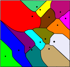
Figure 3. An example related to Lemma 5.1 in a square in $(\mathbb{R}^{2},\ell_{7})$. Here $p=p_{k}$, $A$ is the collection of the other singleton sites $p_{j},j\neq k$, and $\textnormal{dom}(p,A)$ is the Voronoi cell of $p_{k}$. The set $B_{p}$ is simply the unit ball.

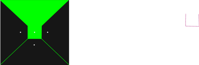
Figure 4. An example where the conclusion of Lemma 5.1 fails if the uniform convexity assumption is removed. Here $X$ is a square in $(\mathbb{R}^{2},\ell_{\infty})$, $p=(0,0)$, and $A=\{(2,0),(-2,0),(0,-2)\}$. The green region is $\textnormal{dom}(p,A)$.

An example related to Lemma 5.1 is given in Figure 4. This may be somewhat surprising, but in general the conclusion of Lemma 5.1 is not true, and Figure 4 presents a counterexample in the non-uniformly convex space $(\mathbb{R}^{2},\ell_{\infty}$) with two simple sets.

An examination of the above proof suggests that problems can appear if no positive number $s$ satisfies the condition in the formulation of Lemma 5.1, because in this case the function $f^{-1}$ may not be continuous. Such a phenomenon occurs in infinite dimensional spaces, for instance, when $X$ is the Hilbert cube $I^{\infty}$ in $\ell_{2}$, but cannot happen if $p$ is in the interior of $X$ relative to the closed affine hull spanned by it. In order to replace Lemma 5.1 one has to show directly by other arguments that $\textnormal{dom}(p,A)$ is connected and locally connected. This will be done in Lemma 5.2 below.

Lemma 5.2.

Let $X$ be a closed and convex set in a uniformly convex normed space. Let $p\in X$ and $\emptyset\neq A\subset X$ and suppose that $d(p,A)>0$. Suppose also that condition (3) holds and that $p$ has the emanation property. Then $\textnormal{dom}(p,A)$ is path connected and locally path connected.

Proof.

By Lemma 4.2, any two points $x_{1},x_{2}\in\textnormal{dom}(p,A)$ can be connected via $p$, so $\textnormal{dom}(p,A)$ is path connected. In order to prove that $\textnormal{dom}(p,A)$ is locally path connected it suffices by Lemma 4.6 to show that it is weakly locally path connected. Let $x_{0}\in\textnormal{dom}(p,A)$. If $x_{0}=p$, then let $V=B(x_{0},r)\cap X$ for $r=d(p,A)/3$. Given $y\in V$, the triangle inequality shows that $3r=d(p,A)\leq d(p,y)+d(y,A)\leq r+d(y,A)$. Hence $d(y,p)\leq r<2r\leq d(y,A)$ and $y\in\textnormal{dom}(p,A)$, so $V\subseteq\textnormal{dom}(p,A)$. Since $V$ is convex, $x_{0}=p$ has a path connected open neighborhood.

Now suppose that $x_{0}\neq p$, and for any $\epsilon>0$ let $U=B(x_{0},\epsilon)\cap\textnormal{dom}(p,A)$ be any neighborhood of $x_{0}$. Let $\theta_{0}=(x_{0}-p)/|x_{0}-p|$. Then $|\theta_{0}|=1$, and since $x_{0}=p+|x_{0}-p|\theta_{0}\in\textnormal{dom}(p,A)$, the definition of $T(\theta_{0},p)$ (in (2)) implies that $d(x_{0},p)\leq T(\theta_{0},p)$. Hence $x^{\prime}_{0}:=(x_{0}-p)/T((x_{0}-p)/|x_{0}-p|,p)=(|x_{0}-p|/T(\theta_{0},p))\theta_{0}$ is well defined, different from 0 and belongs to $B_{p}=\{r\theta:r\in[0,1],\,|\theta|=1,\,\,p+t\theta\in X\,\textnormal{for some}\,\,t>0\}$. In addition, $|x^{\prime}|>0$ for each $x^{\prime}\in B(x^{\prime}_{0},|x^{\prime}_{0}|/2)\cap B_{p}$.

Define $f:B(x^{\prime}_{0},|x^{\prime}_{0}|/2)\cap B_{p}\to\textnormal{dom}(p,A)$ by $f(x^{\prime})=p+T(x^{\prime}/|x^{\prime}|,p)x^{\prime}$. Since $T(\cdot,p)$ is continuous (Theorem 4.4) and since $f(x^{\prime}_{0})=x_{0}$, it follows that $f$ is continuous, so for the given $\epsilon>0$, there exists some $\delta_{1}\in(0,|x^{\prime}_{0}|/2)$ such that if $|x^{\prime}-x^{\prime}_{0}|<\delta_{1}$, then $|f(x^{\prime})-f(x^{\prime}_{0})|<\epsilon$. Hence $f(U^{\prime}_{1})\subset U$ for $U^{\prime}_{1}=B(x^{\prime}_{0},\delta_{1})\cap B_{p}$. Since $U^{\prime}_{1}$ is a path connected (in fact, convex) open set containing $x^{\prime}_{0}$, the continuity of $f$ implies that $f(U^{\prime}_{1})$ is a path connected set contained in $U$ and containing $x_{0}=f(x^{\prime}_{0})$. In order to establish the weak (path) connectedness of $\textnormal{dom}(p,A)$, it suffices to show that $f(U^{\prime}_{1})$ contains an open neighborhood of $x_{0}$.

Since $T(\theta_{0},p)>0$, the continuity of $T(\cdot,p)$ implies that there exists $\delta_{2}\in(0,1)$ such that if $\theta\in\Theta_{p}$ and $|\theta-\theta_{0}|<\delta_{2}$, then $T(\theta,p)>0$. Let $\delta_{3}=\delta_{2}|x_{0}-p|/2$. Given $x\in B(x_{0},\delta_{3})\cap\textnormal{dom}(p,A)$, we have

(4) $$\left|\frac{x-p}{|x-p|}-\frac{x_{0}-p}{|x_{0}-p|}\right|=\frac{\left||x_{0}-p|(x-p)-|x-p|(x_{0}-p)\right|}{|x-p||x_{0}-p|}=\\ \frac{\left|(|x_{0}-p|-|x-p|)(x-p)+|x-p|((x-p)-(x_{0}-p))\right|}{|x-p||x_{0}-p|}\leq\frac{2|x_{0}-x|}{|x_{0}-p|}<\delta_{2}.$$

Thus $T((x-p)/|x-p|,p)>0$ for each $x\in B(x_{0},\delta_{3})\cap\textnormal{dom}(p,A)$. For each such $x$, let $g(x)=(x-p)/T((x-p)/|x-p|,p)$. Since $g$ is continuous, for $\delta_{1}$ from the definition of $U^{\prime}_{1}$ there exists $\delta_{4}\in(0,\delta_{3})$ such that if $|x-x_{0}|<\delta_{4}$, then $|g(x)-g(x_{0})|<\delta_{1}$. But $g(x_{0})=x^{\prime}_{0}$ and $g(x)\in U^{\prime}_{1}$ for each $x$ in the set $V:=B(x_{0},\delta_{4})\cap\textnormal{dom}(p,A)$. In addition, by the definition of $f$ and $g$ we have $x=f(g(x))$ for each $x\in V$ (just let $\theta=(x-p)/|x-p|$ and $x^{\prime}=g(x)$, and note that $x^{\prime}/|x^{\prime}|=\theta$). Hence $V$ is an open neighborhood of $x_{0}$ which is contained in $f(U^{\prime}_{1})$, so $\textnormal{dom}(p,A)$ is weakly locally path connected and hence locally path connected by Lemma 4.6. ∎

Lemma 5.3.

Let $X$ be a closed and convex subset of a uniformly convex normed space. Let $P=\{p_{1},\ldots,p_{m}\}\subset X$ and assume that $\emptyset\neq A\subset X$ satisfies $d(P,A)>0$. Suppose also that condition (3) holds and that the subset $P$ has the emanation property. Then $\textnormal{dom}(P,A)$ is locally path connected.

Proof.

This assertion is a simple consequence of the facts that $\textnormal{dom}(P,A)=\bigcup_{i=1}^{m}\textnormal{dom}(p_{i},A))$ (by Lemma 4.9), that $\textnormal{dom}(p_{i},A)$ is locally path connected (by Lemma 5.2) and closed for each $i$, and the fact that the metric space $\textnormal{dom}(P,A)$ is a finite union of locally path connected closed sets and hence locally path connected by Lemma 4.7. Note that the topology of $\textnormal{dom}(p_{i},A)$, which is induced by the norm of the space, coincides with its topology as a subspace of $\textnormal{dom}(P,A)$, and hence we can apply Lemma 4.7. ∎

Proposition 5.4.

Let $X$ be a compact and convex subset of a uniformly convex normed space, and let $(P_{k})_{k\in K}$ be a finite tuple of finite sets in $X$ which are pairwise disjoint. Suppose that for each $k\in K$ the site $P_{k}$ has the emanation property. For each $k\in K$, let $A_{k}=\bigcup_{j\neq k}P_{j}$ and $Q_{k}=\textnormal{dom}(P_{k},A_{k})$. Let $Y_{k}=\{C:\,C\,\,\textnormal{is closed}\,\,\textnormal{and}\,\,P_{k}\subseteq C\subseteq Q_{k}\}$, endowed with the Hausdorff metric. Let $Y=\prod_{k\in K}Y_{k}$, endowed with the uniform Hausdorff metric. Then $Y\approx I^{\infty}$.

Proof.

Given $k\in K$ and $p\in P_{k}$, let $C_{p}$ be the path connected component of $p$ in $Q_{k}$, and let $E_{p}=\{q\in P_{k}:q\in C_{p}\}$. Since $d(P_{k},A_{k})>0$ for each $k$ by assumption, we have $d(q,A_{k})>0$ for any $q\in E_{p}$, so $\textnormal{dom}(q,A_{k})$ is path connected by Lemma 5.2. Thus $\textnormal{dom}(q,A_{k})\subseteq C_{p}$ for each $q\in E_{p}$, and hence $\textnormal{dom}(E_{p},A_{k})\subseteq C_{p}$ by Lemma 4.9. On the other hand, if $x\in C_{p}$, then $x\in\textnormal{dom}(p^{\prime},A_{k})$ for some $p^{\prime}\in P_{k}$, because $Q_{k}=\bigcup_{p\in P_{k}}\textnormal{dom}(p,A_{k})$ by Lemma 4.9. Lemma 5.2 implies that there is a path between $p^{\prime}$ and $x$, and since $x\in C_{p}$, there is a path between $x$ and $p$. Thus $p^{\prime}\in E_{p}$, so $x\in\textnormal{dom}(p^{\prime},A_{k})\subseteq\textnormal{dom}(E_{p},A_{k})$ and hence $\textnormal{dom}(E_{p},A_{k})=C_{p}$.

Since for each $p_{1},p_{2}\in P_{k}$, either $E_{p_{1}}=E_{p_{2}}$ or $E_{p_{1}}\cap E_{p_{2}}=\emptyset$, it follows that $\{E_{p}:p\in P_{k}\}=\{E_{k,1},\ldots,E_{k,m_{k}}\}$ for some disjoint sets $E_{k,l},\,l=1,\ldots,m_{k}$, the union of which is $P_{k}$. Hence the path connected components of $Q_{k}$ are $\textnormal{dom}(E_{k,1},A_{k}),\ldots,\textnormal{dom}(E_{k,m_{k}},A_{k})$, and since they are closed and disjoint in the compact set $X$, they are, in fact, compact and positively separated. Since $E_{k,l}\subseteq P_{k}$, we have $d(E_{k,l},A_{k})\geq d(P_{k},A_{k})>0$ for each $k$ and each $l$. Hence, by Lemma 5.3, the sets $\textnormal{dom}(E_{k,l},A_{k})$ are also locally path connected.

By Lemma 4.8, we have $E_{k,l}\varsubsetneqq\textnormal{dom}(E_{k,l},A_{k})$ for each $l=1,\ldots,m_{k}$ and each $k$, because there are points $x$ with $d(x,E_{k,l})=r/4$ for $r=d(E_{k,l},A_{k})$ and each such point is in $\textnormal{dom}(E_{k,l},A_{k})$, but not in $E_{k,l}$. Consequently, Theorem  3.2 implies that $2^{\textnormal{dom}(E_{k,l},A_{k})}_{E_{k,l}}\approx I^{\infty}$. Using the fact that the sets $\textnormal{dom}(E_{k,1},P_{k})$, $\textnormal{dom}(E_{k,2},P_{k})$,$\ldots,\textnormal{dom}(E_{k,m_{k}},P_{k})$ are positively separated (and also the fact that any closed set $C$ in $Y_{k}$ has the unique decomposition $C=\bigcup_{l=1}^{m_{k}}(C\cap\textnormal{dom}(E_{k,l},A_{k}))$ as a disjoint union of closed sets contained in the components $\textnormal{dom}(E_{k,l},A_{k})$), we can easily verify that $Y_{k}$ with the Hausdorff metric is homeomorphic to the finite product space $\prod_{l=1}^{m_{k}}2^{\textnormal{dom}(E_{k,l},A_{k})}_{E_{k,l}}$, endowed with the uniform Hausdorff metric. Therefore $Y_{k}\approx(I^{\infty})^{m_{k}}\approx I^{\infty}$, and hence $Y\approx I^{\infty}$. ∎

6. Continuity of the Dom mapping

Proposition 6.1.

Let $X$ be a convex subset of a uniformly convex normed space, and let $(P_{k})_{k\in K}$ be a tuple of nonempty and positively separated sets in $X$, that is, $\inf\{d(P_{k},P_{j}):j,k\in K,j\neq k\}>0$. Assume that condition (3) holds (with the same $\rho$) for each $k\in K$ with $P_{k}$ and $A_{k}=\bigcup_{j\neq k}P_{j}$ instead of $P$ and $A$. Suppose that the distance between each $x\in X$ and each $P_{k},\,k\in K$, is attained. For each $k\in K$ let $Q_{k}=\textnormal{dom}(P_{k},\bigcup_{j\neq k}P_{j})$ and $Y_{k}=\{C:\,\,C\,\textnormal{is closed}\,\,\textnormal{and}\,\,P_{k}\subseteq C\subseteq Q_{k}\}$. Let $Y=\prod_{k\in K}Y_{k}$, endowed with the uniform Hausdorff metric $\widetilde{D}$ defined by $\widetilde{D}((S_{k})_{k\in K},(S^{\prime}_{k})_{k\in K})=\sup\{D(S_{k},S^{\prime}_{k}):k\in K\}$. Then Dom maps $Y$ into itself and is uniformly continuous there.

Proof.

First, note that for any nonempty subsets $P,A,B$ of $X$, if $A\subseteq B$, then $\textnormal{dom}(P,B)\subseteq\textnormal{dom}(P,A)$. Now let $S=(S_{k})_{k\in K}\in Y$ be given. By the definition of $Y_{k}$, we have $P_{k}\subseteq S_{k}$ for each $k\in K$, so $W_{k}:=\textnormal{dom}(P_{k},\bigcup_{j\neq k}S_{j})\subseteq\textnormal{dom}(P_{k},\bigcup_{j\neq k}P_{j})=Q_{k}$ by the definition of $Q_{k}$. Since the $k$-th component of $W:=\textnormal{Dom}(S)$ is the closed subset $W_{k}$, we conclude that $(P_{k})_{k\in K}\subseteq\textnormal{Dom}(S)\subseteq(Q_{k})_{k\in K}$, and hence Dom maps $Y$ into itself.

Now let $\epsilon>0$ satisfy $12\epsilon\leq\inf\{d(P_{k},P_{j}):j,k\in K,j\neq k\}$, and let $\Delta$ correspond to $\epsilon$ in Theorem 4.3. Let $S=(S_{k})_{k\in K},S^{\prime}=(S^{\prime}_{k})_{k\in K}$ be any two tuples in $Y$ satisfying $\widetilde{D}(S,S^{\prime})<\Delta$. As a result, we also have $D(S_{k},S^{\prime}_{k})<\Delta$ for each $k\in K$. This implies that $D(\bigcup_{j\neq k}S_{j},\bigcup_{j\neq k}S^{\prime}_{j})\leq\Delta$ for each $k\in K$, because $D(\bigcup_{j\neq k}S_{j},\bigcup_{j\neq k}S^{\prime}_{j})\leq\sup\{D(S_{j},S^{\prime}_{j}):j\neq k\}$.

Fix $k\in K$. If $x\in\bigcup_{j\neq k}S_{j}$, then $x\in S_{j}$ for some $j\neq k$, so $x\in Q_{j}=\textnormal{dom}(P_{j},\bigcup_{i\neq j}P_{i})\subseteq\textnormal{dom}(P_{j},P_{k})$. Hence $d(x,P_{k})\geq 6\epsilon$ by Lemma 4.8. Thus $d(P_{k},\bigcup_{j\neq k}S_{j})\geq 6\epsilon$ for each $k\in K$. Hence all the conditions of Theorem 4.3 are satisfied (here $P=P_{k}=P^{\prime}$, $A=\bigcup_{j\neq k}S_{j}$, $A^{\prime}=\bigcup_{j\neq k}S^{\prime}_{j}$ and condition (3) of Theorem 4.3 for $A$ follows from condition (3) for $A_{k}=\bigcup_{j\neq k}P_{j}$ because $P_{j}\subseteq S_{j}$). Thus $D(\textnormal{dom}(P_{k},\bigcup_{j\neq k}S_{j}),\textnormal{dom}(P_{k},\bigcup_{j\neq k}S^{\prime}_{k}))<\epsilon$ for each $k\in K$. By the definition of Dom and $\widetilde{D}$, we have $\widetilde{D}(\textnormal{Dom}(S),\textnormal{Dom}(S^{\prime}))\leq\epsilon$, so Dom is indeed uniformly continuous on $Y$. ∎

7. The main result

Proposition 7.1.

Let $X$ be a compact and convex subset of a uniformly convex normed space, and let $(P_{k})_{k\in K}$ be a finite tuple of finite sets in $X$ which are pairwise disjoint. Suppose that for each $k\in K$, the site $P_{k}$ has the emanation property. Then there exists a zone diagram with respect to these sites.

Proof.

Given the finite sites $(P_{k})_{k\in K}$, let $Y$ be as in Proposition 6.1. Since Dom maps $Y$ into itself and is continuous there by Propostion 6.1, and since $Y$ is homeomorphic to the Hilbert cube by Proposition 5.4, we deduce the existence of a zone diagram from the Schauder fixed point theorem, as explained in the beginning of Section 3. ∎

Theorem 7.2.

Let $X$ be a compact and convex subset of a uniformly convex normed space, and let $(P_{k})_{k\in K}$ be a finite tuple of compact sets in $X$ which are pairwise disjoint. Suppose that for each $k\in K$, the site $P_{k}$ has the emanation property. Then there exists a zone diagram with respect to these sites.

Proof.

Let $(P_{k})_{k\in K}$ be the given finite tuple of pairwise disjoint compact sites. Let $r=\min\{d(P_{k},P_{j}):j\neq k\}$. By the compactness of the sites, for each positive integer $m$ and for each $k\in K$, there exists a finite subset $P_{m,k}$ of $P_{k}$ such that $D(P_{m,k},P_{k})<1/m$. Note that $d(P_{m,k},P_{m,j})\geq r$ whenever $j\neq k$. For each $m$, let $R_{m}=(R_{m,k})_{k\in K}$ be a zone diagram corresponding to the tuple $(P_{m,k})_{k\in K}$, the existence of which is guaranteed by Proposition 7.1. In other words,

(5) $$R_{m,k}=\textnormal{dom}(P_{m,k},\bigcup_{j\neq k}R_{m,j})\quad\forall k\in K.$$

Since the space of all nonempty compact subsets of $X$ (endowed with the Hausdorff metric) is compact [13], and since $K$ is finite, we can find a convergent subsequence of the finite sites and the components of the corresponding zone diagrams. Therefore for some subsequence $(m_{l})_{l=1}^{\infty}$ of positive integers the sequence $(R_{m_{l},k})_{l=1}^{\infty}$ converges to some set $R_{k}$, and the sequence $(P_{m_{l},k})_{l=1}^{\infty}$ converges to $P_{k}$ by the definition of $P_{m,k}$. Hence $\bigcup_{j\neq k}R_{m_{l},j}$ converges to $\bigcup_{j\neq k}R_{j}$, because $D(\bigcup_{j\neq k}R_{m_{l},j},\bigcup_{j\neq k}R_{j})\leq\max\{D(R_{m_{l},j},R_{j}):j\neq k\}$.

Let $\epsilon^{\prime}=r/12$. Then $12\epsilon^{\prime}\leq\min\{d(P_{m_{l},k},P_{m_{l},j}):j\neq k\}$. Let $k\in K$. If $j\neq k$ and $x\in\bigcup_{j\neq k}R_{m_{l},j}$, then $x\in R_{m_{l},j}$ for some $j\neq k$. Therefore

$$x\in\textnormal{dom}(P_{m_{l},j},\bigcup_{i\neq j}R_{m_{l},i})\subseteq\textnormal{dom}(P_{m_{l},j},\bigcup_{i\neq j}P_{m_{l},i})\subseteq\textnormal{dom}(P_{m_{l},j},P_{m_{l},k}).$$

Hence $d(x,P_{m_{l},k})\geq 6\epsilon^{\prime}$ by Lemma 4.8, and, as a result, $d(P_{m_{l},k},\bigcup_{j\neq k}R_{m_{l},j})\geq 6\epsilon^{\prime}$ for each $k\in K$ and $l$. Thus $d(P_{k},\bigcup_{j\neq k}R_{j})\geq 6\epsilon^{\prime}$ and hence the positive distance condition in Theorem 4.3 holds. From (5) and the continuity of $\textnormal{dom}(\cdot,\cdot)$ (Theorem  4.3) we conclude that $R=(R_{k})_{k\in K}$ is a zone diagram with respect to $(P_{k})_{k\in K}$. ∎

The hypotheses of Theorem 7.2 are satisfied, in particular, when all the compact sites are contained in the interior of a closed ball (or another compact and convex set) in $\mathbb{R}^{n}$.

8. Concluding remarks and open problems

In this short section we describe several interesting questions and directions for further investigation.

An interesting problem is whether the dominance region $\textnormal{dom}(P,A)$ is locally connected for general positively separated sets $P$ and $A$. If so, then this will suggest an alternative method for proving the existence of a zone diagram with respect to compact sites. Second, it would be interesting to extend the existence result further, say to all normed spaces, without any compactness requirement on the sites and the subset $X$. The question of uniqueness is interesting too. It seems that the uniform convexity assumption on the norm is not sufficient even in the plane with two singleton sites, as shown in [15], but perhaps, following [15], uniform convexity combined with uniform smoothness of the norm will imply uniqueness in the infinite dimensional case too. It would also be of interest to establish our main theorem (Theorem 7.2) and auxiliary results (e.g., Lemmata 5.1 and 5.2) without imposing the condition of the emanation property on the points.

Another interesting and natural problem is how to approximate a zone diagram in the setting described in this paper. It turns out that there is a way to do it, and a key point in carrying out this task is to use the algorithm for computing Voronoi diagrams of general sites in general spaces described in [19, 20]. For the sake of completeness, we include two pictures of zone diagrams in the plane with two different norms.

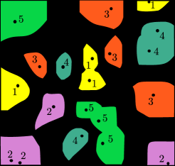
Figure 5. A zone diagram of 5 sites, each with 4 points, in a square in $(\mathbb{R}^{2},\ell_{6})$.

Figure 6. A zone diagram of 3 sites in a square in $(\mathbb{R}^{2},\ell_{p}),\,p=3.14159$, each with 3 points.

The proof of Theorem  7.2 shows that one can approximate the given compact sites by finite subsets of them and then the corresponding zone diagram approximates the real one. Unfortunately, no error estimates are obtained in the proof, and it would indeed be of interest to find such estimates.
Acknowledgements
We thank Akitoshi Kawamura, Jiří Matoušek, and Takeshi Tokuyama for providing a copy of their recent paper [15] before posting it on the arXiv. The first author was supported by Grant FWF-P19643-N18. The third author was partially supported by the Israel Science Foundation (Grant 647/07), the Fund for the Promotion of Research at the Technion (Grant 2001893), and by the Technion President’s Research Fund (Grant 2007842). All the authors thank Orr Shalit and the referee for their helpful suggestions and corrections. We are very grateful to Eva Goldman for kindly redrawing the figures so expertly.

References

- [1] T. Asano and D. Kirkpatrick, Distance trisector curves in regular convex distance metrics, Proceedings of the 3rd International Symposium on Voronoi Diagrams in Science and Engineering (ISVD 2006), pp. 8–17.
- [2] T. Asano, J. Matoušek, and T. Tokuyama, The distance trisector curve, Adv. Math. 212 (2007), 338–360, a preliminary version in STOC 2006, pp. 336- 343.
- [3] by same author, Zone diagrams: Existence, uniqueness, and algorithmic challenge, SIAM J. Comput. 37 (2007), no. 4, 1182–1198, a preliminary version in SODA 2007, pp. 756-765.
- [4] T. Asano and T. Tokuyama, Drawing equally-spaced curves between two points, Abstracts of the 14th Annual Workshop on Computational Geometry with a Focus on Open Problems, 2004, pp. 24–25.
- [5] F. Aurenhammer, Voronoi diagrams - a survey of a fundamental geometric data structure, ACM Computing Surveys, vol. 3, 1991, pp. 345–405.
- [6] J. Chun, Y. Okada, and T. Tokuyama, Distance trisector of segments and zone diagram of segments in a plane, Proceedings of the 4th International Symposium on Voronoi Diagrams in Science and Engineering (ISVD 2007), pp. 66–73.
- [7] J. A. Clarkson, Uniformly convex spaces, Trans. Amer. Math. Soc. 40 (1936), 396–414.
- [8] D. W. Curtis and R. M. Schori, Hyperspaces of Peano continua are Hilbert cubes, Fund. Math. 101 (1978), no. 1, 19–38.
- [9] S. C. de Biasi, B. Kalantari, and I. Kalantari, Maximal zone diagrams and their computation, Proceedings of the 7th international symposium on Voronoi Diagrams in Science and Engineering (ISVD 2010), pp. 171–180.
- [10] J. Dugundji and A. Granas, Fixed point theory, Springer Monographs in Mathematics, Springer-Verlag, New York, 2003.
- [11] K. Goebel and S. Reich, Uniform convexity, hyperbolic geometry, and nonexpansive mappings, Monographs and Textbooks in Pure and Applied Mathematics, vol. 83, Marcel Dekker Inc., New York, 1984.
- [12] C. Gold, The Voronoi Web Site, 2008, http://www.voronoi.com/wiki/index.php?title=Main˙Page.
- [13] A. Illanes and S. B. Nadler Jr, Hyperspaces. Fundamentals and recent advances, Monographs and Textbooks in Pure and Applied Mathematics, vol. 216, Marcel Dekker Inc., New York, 1999.
- [14] K. Imai, A. Kawamura, J. Matoušek, Y. Muramatsu, and T. Tokuyama, Distance k-sectors and zone diagrams, Extended abstract in EuroCG 2009, pp. 191–194. Available at http://www.cs.toronto.edu/~kawamura/publ/090317.
- [15] A. Kawamura, J. Matoušek, and T. Tokuyama, Zone diagrams in Euclidean spaces and in other normed spaces, Mathematische Annalen, to appear. Preliminary versions in SoCG 2010, pp. 216-221, arXiv 0912.3016 (2009).
- [16] J. Lindenstrauss and L. Tzafriri, Classical Banach spaces, II: Function spaces, Springer, Berlin, 1979.
- [17] J. Munkres, Topology, second ed., Prentice Hall, Upper Saddle River, NJ, 2000.
- [18] A. Okabe, B. Boots, K. Sugihara, and S. N. Chiu, Spatial tessellations: concepts and applications of Voronoi diagrams, second ed., Wiley Series in Probability and Statistics, John Wiley & Sons Ltd., Chichester, 2000, with a foreword by D. G. Kendall.
- [19] D. Reem, An algorithm for computing Voronoi diagrams of general generators in general normed spaces, Proceedings of the sixth international symposium on Voronoi diagrams in science and engineering (ISVD 2009), pp. 144–152.
- [20] by same author, Voronoi and zone diagrams, Ph.D. thesis, The Technion, Haifa, 2010.
- [21] by same author, The geometric stability of Voronoi diagrams with respect to small changes of the sites, (2011), Complete version in arXiv 1103.4125, Extended abstract in SoCG 2011, pp. 254-263.
- [22] D. Reem and S. Reich, Zone and double zone diagrams in abstract spaces, Colloquium Mathematicum 115 (2009), 129–145, arXiv 0708.2668 (2007).
- [23] J. Schauder, Der Fixpunktsatz in Funktionalräumen, Studia Math. 2 (1930), 171–180.
- [24] T. Zamfirescu, Typical starshaped sets, Aequ. Math. 36 (1988), 188–200.