Enhanced relativistic harmonics by electron nanobunching

Abstract

It is shown that when an few-cycle, relativistically intense, $p$-polarized laser pulse is obliquely incident on overdense plasma, the surface electrons may form ultra-thin, highly compressed layers, with a width of a few nanometers. These electron “nanobunches” emit synchrotron radiation coherently. We calculate the one-dimensional synchrotron spectrum analytically and obtain a slowly decaying power-law with an exponent of $4/3$ or $6/5$. This is much flatter than the $8/3$ power of the BGP (Baeva-Gordienko-Pukhov) spectrum, produced by a relativistically oscillating bulk skin layer. The synchrotron spectrum cut-off frequency is defined either by the electron relativistic $\gamma$-factor, or by the thickness of the emitting layer. In the numerically demonstrated, locally optimal case, the radiation is emitted in the form of a single attosecond pulse, which contains almost the entire energy of the full optical cycle.

I Introduction

High harmonics generated by an intense laser pulse incident on an overdense plasma surface are a promising bright source of short wavelength radiation with a number of potential applications PukhovNatPhys2006 . Because of the coherent character of the process, the generated harmonics are locked in phase and emerge in the form of attosecond pulses. This could recently also be shown experimentally NomuraNatPhys2009 . Commonly, two mechanisms that lead to harmonics generation from solid density plasma surfaces are distinguished: coherent wake emission (CWE) quere:125004 and the “relativistically oscillating mirror” (ROM) lichters:3425 .

CWE is predominant at moderately relativistic intensities $a_{0}\sim 1$ and short, but finite plasma gradient lengths $\nabla N/N\sim 0.01\,\lambda$. Here, $a_{0}=eA/mc^{2}$ is the relativistically normalized laser potential. In this regime the Brunel electrons that re-enter the plasma excite electrostatic oscillations in the overcritical plasma regions. Because of the strong density inhomogeneity, the electrostatic oscillations couple back to electromagnetic modes and thus generate harmonics. Due to this mechanism, CWE spectra have a cut-off at the plasma frequency corresponding to the maximum density. Further, the harmonics have a comparatively wide emission cone Dromey2009 .

ROM harmonics dominate for $a_{0}\gg 1$, although recent studies tarasevitch:103902 have shown that they can be observed even at lower intensities when the plasma gradient length is about $\nabla N/N\sim 0.1\,\lambda$. ROM spectra have no cut-off at the plasma frequency, but can extend to much higher frequencies. Their origin is basically the relativistic non-linearity in the electron motion. Baeva, Gordienko and Pukhov (BGP) bgp-theory2006 have developed a theory to analytically describe the spectrum in this highly relativistic regime. The BGP harmonic spectrum is a power law with the exponent $-8/3$, smoothly rolling off into an exponential decay at some frequency scaling as $I^{3/2}$. This type of spectrum could be observed experimentally Dromey2006 .

So far these two mechanisms have been the widely accepted explanations for harmonics generation at overdense plasma surfaces. However, there has also been some evidence that the two models do not tell the whole story. Especially under $p$-polarized oblique incidence, with $a_{0}\gg 1$ some spectra could be observed in numerical simulations boyd:125004 that do not fit to the predictions of neither of the models.

In this paper, we take the most general approach to describe the harmonics radiation of the relativistic electrons: It is described as coherent synchrotron emission of the one dimensional slab geometry electron distribution. For synchrotron radiation, the optimal efficiency is reached, when all the radiating electrons gather in one extremely dense and narrow bunch. We demonstrate via PIC simulation, that this case can actually closely be achieved in relativistic laser-plasma interaction.

II Assumptions and Predictions of BGP Theory

We start with a brief review of the BGP theory. The theory is one dimensional, oblique incidence can be treated in a Lorentz transformed frame Bourdier1983 . This is acceptable as long as the focal spot size is big compared to the laser wavelength adBPuk2007 . The reflection of the light is done by the electrons close to the surface. In general, the surface electrons perform highly complicated motions and it is a hopeless endeavour to try to describe it analytically even in 1D. Therefore we have to resort to some approximation. The starting point of the BGP model is the following, simplified boundary condition:

$$E_{i}\left(t-x_{\textrm{ARP}}(t)/c\right)+E_{r}\left(t+x_{\textrm{ARP}}(t)/c\right)=0$$ (1)

where $x_{\textrm{ARP}}$ is the so called “Apparent Reflection Point” (ARP) position (see Eq. (18) in bgp-theory2006 ). The whole information about the plasma motion has been condensed to only one real function $x_{\textrm{ARP}}(t)$. However, we have to emphasize here, that Eq. (1) is an approximation. Although it is not yet possible to give a fully general criterion for the validity of Eq. (1) in terms of the initial laser and plasma parameters, it has been demonstrated in PhysRevLett.93.115002 that the approximation is valid if the plasma skin layer evolution time $\tau$ is long compared to the skin length $\delta$ in the sense $c\tau\gg\delta$ . This is the case if $S\equiv N_{e}/a_{0}N_{c}\gg 1$, or generally if the electron density profile is approximately step-like during the main interaction phase.

Further note that Eq. (1) makes sense only for an ARP moving at a physical velocity of $|\dot{x}_{\textrm{ARP}}|<c$. In this case it is clear from Eq. (1), that the reflected field is nothing but a phase modulation of the negative of the incident field. This can easily be checked inside a PIC simulation. Fig. 1a shows an exemplary result. For this simulation, the laser was normally incident on a sharp edged plasma density profile. Here, Eq. (1) is fulfilled to a good approximation as can be verified from Fig. 1a: Apart from minor deviations, the extremal values and the sequence of the monotonic intervals agree, the reflected field is approximately a phase modulation of the incident one.

Starting from Eq. (1), it is now possible to calculate the spectrum of the reflected radiation with only little knowledge of the function $x_{\textrm{ARP}}(t)$. Therefore we perform the Fourier transformation of $E_{r}(t)$ employing the method of stationary phase. At the stationary phase point, the relativistic $\gamma$-factor corresponding to the ARP $\gamma_{\textrm{ARP}}=(1-(\min(\dot{x}_{\textrm{ARP}}/c))^{2})^{-1/2}$ possesses an extremely sharp maximum, why we also refer to this point as the $\gamma$-spike. The high frequency spectrum does only depend on the surface behavior near this $\gamma$-spike. Therefore, we can also relax the condition for the validity of the theory: Actually, we require Eq. (1) only to be fulfilled in the neighbourhood of the $\gamma$-spike.

The exact result of the calculation of the spectrum is given by Eqs. (34)-(36) in bgp-theory2006 , in a very good approximation it can be simplified to:

$$I(\omega)\propto\frac{1}{\omega^{8/3}}\,\left[\textrm{Ai}\left(\left(\frac{\omega}{\omega_{r}}\right)^{2/3}\right)\right]^{2}$$ (2)

wherein Ai refers to the well known Airy-function. The roll-off frequency $\omega_{r}$ marks the point, where the initial power law decay of the spectral envelope merges into a more rapid exponential decay. In the region $\omega\ll\omega_{r}$, the Airy function is $O(1)$ and one obtains the $-8/3$-power law spectrum. For $\omega\gg\omega_{r}$, the decay is an exponential one. From the integration, it also follows that $\omega_{r}\propto\gamma_{\textrm{ARP}}^{3}$, where $\gamma_{\textrm{ARP}}$ is taken at its maximum. The scaling with $\gamma_{\textrm{ARP}}^{3}$ is in contrast to the long known case of reflection at a mirror moving with constant velocity generates a Doppler upshift of only $(1+\beta)/(1-\beta)\approx 4\gamma^{2}$.

Fig. 1b shows the spectrum corresponding to the field from Fig. 1a. As expected, it agrees well with the $-8/3$-power law.

III A New Regime of Relativistic Harmonics Generation

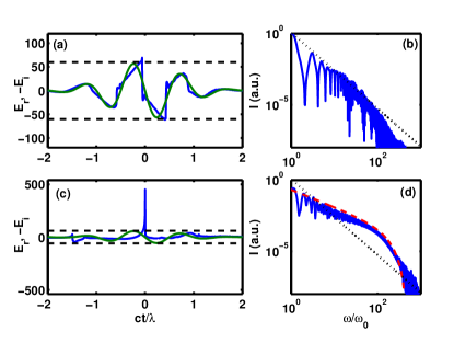
Figure 1: Radiation in time ((a) and (c)) and spectral ((b) and (d)) domain for two simulations. (a) and (b) correspond to the BGP case: normal incidence, plasma density $N_{e}=250\,N_{c}$, sharp edged profile; (c) and (d) correspond to the nanobunching case: plasma density ramp $\propto\exp(x/(0.33\,\lambda))$ up to a maximum density of $N_{e}=95\,N_{c}$ (lab frame), oblique incidence at $63^{\circ}$ angle ($p$-polarized). Laser field amplitude is $a_{0}=60$ in both cases. In all frames, the reflected field is represented by a blue line. In (a) and (c), the green line represents the field of the incident laser and the black dashed lines mark the maximum field of it. In (b) and (d), the dotted black line represents an $8/3$ power law, the red dashed line corresponds to the 1D synchrotron spectrum Eqs. (6) and (7), with $\omega_{rs}=800\,\omega_{0}$ and $\omega_{rf}=225\,\omega_{0}$.

Let us now have a look at Fig. 1c, which shows the result of another PIC simulation. In this simulation the plasma density profile was extended over a few fractions of a laser wavelength, and the $p$-polarized laser was incident at an angle of $\alpha=63^{\circ}$. The laser pulse used was the same as in the first simulation.

It is evident, that the maximum of the reflected field reaches out about an order of magnitude above the amplitude of the incident laser. The reflected radiation can clearly not be obtained from the incident one just by phase modulation. By this we conclude, that the boundary condition Eq. (1) fails here. Consequently, the spectrum deviates from the $-8/3$-power law, compare Fig. 1d. Indeed we see that the efficiency of harmonic generation is much higher than estimated by the BGP calculations: about two orders of magnitude at the hundredth harmonic. Also, we can securely exclude CWE as the responsible mechanism, since this would request a cut-off around $\omega=10\omega_{0}$. From this we conclude that the radiation cannot be attributed to any of the known mechanisms.

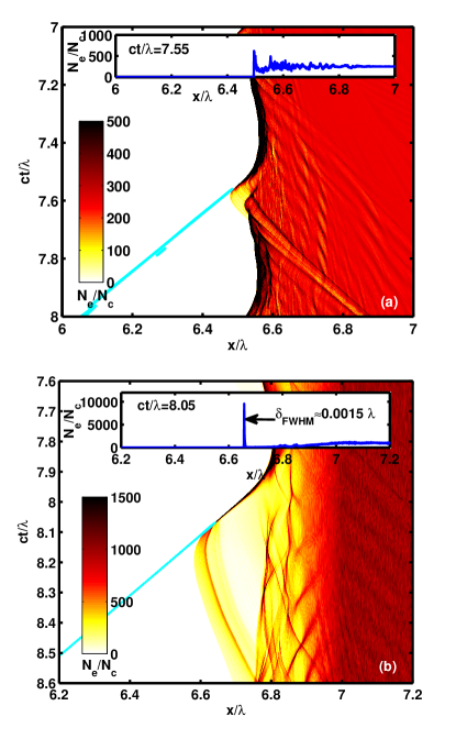
Figure 2: (Color online) The electron density and contour lines (cyan, or light grey) of the emitted harmonics radiation for $\omega/\omega_{0}>4.5$, in (a) the BGP and (b) the synchrotron (or nanobunching) regime. The small windows inside the main figures show the detailed density profile at the instant of harmonic generation. All magnitudes are taken in the simulation frame. The parameters used are the same as in the other figures.

To get a picture of the physics behind, let us have a look at the motion of the plasma electrons that generate the radiation. Figure 2 shows the evolution of the electron density in both our sample cases. In addition to the density, contour lines of the spectrally filtered reflected radiation are plotted. These lines illustrate where the main part of the high frequency radiation emerges. We observe that in both cases the main part of the harmonics is generated at the point, when the electrons move towards the observer. This shows again that in both cases the radiation does not stem from CWE. For CWE harmonics, the radiation is generated inside the plasma, at the instant when the Brunel electrons re-enter the plasma quere:125004 . Apart from that mutuality, the two presented cases appear to be very different.

Figure 2a corresponds to the BGP case. It can be seen that the density profile remains roughly step-like during the whole interaction process and the plasma skin layer radiates as a whole. This explains why the BGP theory works well here, as we have seen before in Fig. 1a and b.

However, figure 2b looks clearly different. The density distribution at the moment of harmonics generation is far from being step-like, but possesses a highly dense (up to $\sim 10000\,N_{c}$ density) and very narrow $\delta$-like peak, with a width of only a few nanometers. This electron “nanobunch” emits synchrotron radiation coherently.

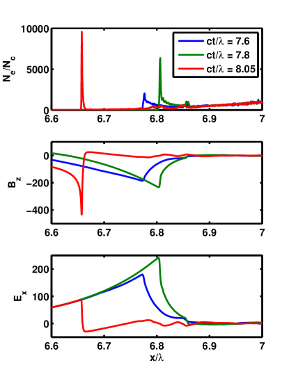
Figure 3: (Color online) Formation of the nanobunch in the simulation corresponding to Figs. 1c-d and 2b. We depict the electron density $N_{e}$ in units of the critical density $N_{c}$, the transverse magnetic field component $B_{z}$ and the longitudinal electric field component $E_{x}$ in relativistically normalized units.

The radiation is emitted by a highly compressed electron bunch moving away from the plasma. However, the electrons first become compressed by the relativistic ponderomotive force of the laser that is directed into the plasma, compare the blue lines in Fig. 3. During that phase, the longitudinal electric field component grows until the electrostatic force turns around the bunch, compare the green lines in Fig. 3. Normally, the bunch will loose its compression in that instant, but in some cases, as in the one considered here, the fields and the bunch current match in a way that the bunch maintains or even increases its compression. The final stage is depicted by the red lines in Fig. 3.

We emphasize, that such extreme nanobunching does not occur in every case of $p$-polarized oblique incidence of a highly relativistic laser on an overdense plasma surface. On the contrary, it turns out that the process is highly sensitive to changes in the plasma density profile, laser pulse amplitude, pulse duration, angle of incidence and even the carrier envelope phase of the laser. For a longer pulse, we may even observe the case, that nanobunching is present in some optical cycles but not in others. The parameters in the example were selected in a way to demonstrate the new effect unambiguously, i.e. the nanobunch is well formed and emits a spectrum that clearly differs from the BGP one. The dependence of the effect on some parameters is discussed in section VI.

Because of the one dimensional slab geometry, the spectrum is not the same as the well known synchrotron spectra Jackson of a point particle. We now calculate the spectrum analytically.

IV Spectrum of 1D Coherent Synchrotron Emission (CSE)

The radiation field generated to the left of a one-dimensional current distribution can in a completely general way be expressed as:

$$E_{sy}\left(t,x\right)=\frac{2\pi}{c}\int_{-\infty}^{+\infty}j\left(t+\frac{x-x^{\prime}}{c},x^{\prime}\right)\,dx^{\prime}$$ (3)

Optimal coherency for high frequencies will certainly be achieved, if the current layer is infinitely narrow: $j(t,x)=j(t)\delta(x-x_{el}(t))$. To include more realistic cases, we allow in our calculations for a narrow, but finite electron distribution:

$$j(t,x)=j(t)f(x-x_{el}(t))$$ (4)

with variable current $j(t)$ and position $x_{el}(t)$, but fixed shape $f(x)$. We take the Fourier transform of Eq. (3), thereby considering the retarded time, and arrive at the integral $\tilde{E}_{sy}(\omega)=2\pi c^{-1}\tilde{f}(\omega)\int j(t)\,\exp\left[-i\omega\left(t+x_{el}(t)/c\right)\right]\,dt$. Here, $\tilde{f}(\omega)$ denotes the Fourier transform of the shape function. In analogy to the standard synchrotron radiation by a point particle, the integral can be solved with the method of stationary phase. Therefore we note, that for high $\omega$ the main contributions to the integral come from the regions, where the phase $\Phi=\omega\left(t+x_{el}(t)/c\right)$ is approximately stationary, i.e. $d\Phi/dt\approx 0$. However, to get some kind of result we need some assumption about the relation between the functions $j(t)$ and $x_{el}(t)$. Since we are dealing with the ultrarelativistic regime $a_{0}\gg 1$, it is reasonable to assume that changes in the velocity components are governed by changes in the direction of movement rather than by changes in the absolute velocity, which is constantly very close to the speed of light $c$.

Let the electron motion in momentum space be given by $\left(p_{x},p_{y}\right)=a_{0}m_{e}c\left(\hat{p}_{x}\,\hat{p}_{y}\right)$, so that $j(t)=ecn_{e}\hat{p}_{y}/(a_{0}^{-2}+\hat{p}_{x}^{2}+\hat{p}_{y}^{2})$ and $\dot{x}_{el}=c\hat{p}_{x}/(a_{0}^{-2}+\hat{p}_{x}^{2}+\hat{p}_{y}^{2})$. The derivative of the phase approaches zero at points where $\dot{x}_{el}\approx-c$, so from our assumption of ultrarelativistic motion we conclude $\hat{p}_{y}=0$ at these instants. Now, two cases have to be distinguished:

1. The current changes sign at the stationary phase point. Then we can Taylor expand $j(t)=\alpha_{0}\,t$ and $x_{el}(t)=-v_{0}t+\alpha_{1}t^{3}/3$. The integral can now be expressed in terms of the well-known Airy-function, yielding $\tilde{E}_{sy}(\omega)=C\,\tilde{f}(\omega)\,\omega^{-2/3}\textrm{Ai}^{\prime}\left(\frac{1-v_{0}}{\sqrt[3]{\alpha_{1}}}\omega^{2/3}\right),$ where $\textrm{Ai}^{\prime}$ is the Airy function derivative and $C=i(2\pi)^{2}en_{e}c^{-1}\alpha_{0}\alpha_{1}^{-2/3}$ is a complex prefactor. We now find the spectral envelope

   $$I(\omega)\propto|\tilde{f}(\omega)|^{2}\,\omega^{-4/3}\,\left[\textrm{Ai}^{\prime}\left(\left(\frac{\omega}{\omega_{rs}}\right)^{2/3}\right)\right]^{2}$$ (5)

   with $\omega_{rs}\approx 2^{3/2}\sqrt{\alpha_{1}}\gamma_{0}^{3}$, where $\gamma_{0}=(1-v_{0}^{2})^{-1/2}$ is the relativistic $\gamma$-factor of the electron bunch at the instant when the bunch moves towards the observer. As in the BGP case, the spectral envelope (5) does not depend on all details of the electron bunch motion $x_{el}$, but only on its behavior close to the stationary points, i.e. the $\gamma$-spikes.

2. The current does not change sign at the stationary phase point. Because of the assumption of highly relativistic motion the changes in absolute velocity can again be neglected compared to the changes in direction, and it follows that in this case the third derivative of $x_{el}$ is zero at the stationary phase point. Therefore, our Taylor expansions look like $j(t)=\alpha_{0}t^{2}$ and $x_{el}(t)=-v_{0}t+\alpha_{1}t^{5}/5$. This leads us to the spectral envelope

   $$I(\omega)\propto|\tilde{f}(\omega)|^{2}\,\omega^{-6/5}\,\left[\textrm{S}^{\prime\prime}\left(\left(\frac{\omega}{\omega_{rs}}\right)^{4/5}\right)\right]^{2}$$ (6)

   with $\textrm{S}^{\prime\prime}$ being the second derivative of $\textrm{S}(x)\equiv(2\pi)^{-1}\int\exp\left[i\left(xt+t^{5}/5\right)\right]\,dt$, a special case of the canonical swallowtail integral 1984Swallowtail . For the characteristic frequency $\omega_{rs}$ we now obtain $\omega_{rs}\approx 2^{5/4}\sqrt[4]{\alpha_{1}}\gamma_{0}^{2.5}$. Because now even the derivative of $\ddot{x}_{el}$ is zero at the stationary phase point, the influence of acceleration on the spectrum decreases and the characteristic frequency scaling is closer to the $\gamma^{2}$-scaling for a mirror moving with constant velocity.

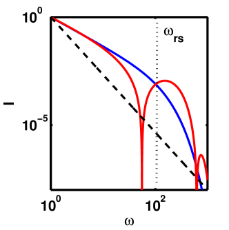
Figure 4: (Color online) Coherent 1D synchrotron spectra for an infinitely thin electron layer $\tilde{f}(\omega)\equiv 1$ and $\omega_{rs}=100$. The blue line corresponds to Eq. (5) and the red line to Eq. (6). For comparison, the dashed black line denotes the BGP $8/3$-power law.

In Fig. 4 the CSE spectra of the synchrotron radiation from the electron sheets are depicted. Comparing them to the $8/3$-power law from the BGP-case, we notice that, because of the smaller exponents of their power law part, the CSE spectra are much flatter, around the 100th harmonic we win more than two orders of magnitude. Another intriguing property are the side maxima found in the spectrum (6). This might provide an explanation for modulations that are occasionally observed in harmonics spectra, compare e.g. Ref. boyd:125004 .

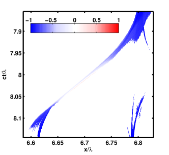
Figure 5: (Color online) Normalized transverse fluid velocity $v_{y}/c$ of the electron nanobunch. Parts of the plasma with a density below $500\,N_{c}$ are filtered out.

To compare with the PIC results, the finite size of the electron bunch must be taken into account. Therefore we assume a Gaussian density profile which leads us to

$$|f(\omega)|^{2}=\exp\left[-\left(\frac{\omega}{\omega_{rf}}\right)^{2}\right]$$ (7)

Thus the spectral cut-off is determined either by $\omega_{rs}$, corresponding to the relativistic $\gamma$-factor of the electrons, or by $\omega_{rf}$ corresponding to the bunch width. A look at the motion of the electron nanobunch in the PIC simulation (Fig. 5) tells us that there is no change in sign of the transverse velocity at the stationary phase point, consequently we use Eq. (6). We choose $\omega_{rf}=225\,\omega_{0}$ and $\omega_{rs}=800\,\omega_{0}$ to fit the PIC spectrum. $\omega_{rf}$ corresponds to a Gaussian electron bunch with a width of $\delta=10^{-3}\lambda$, which matches reasonably well to the $\delta_{FWHM}=0.0015\,\lambda$ (see Fig. 2b) measured in the simulation, corresponding to a Gaussian electron bunch $f(x)=\exp\left[-(x/\delta)^{2}\right]$ with a width of $\delta=10^{-3}\lambda$ and an energy of $\gamma\sim 10$. This matches well with the measured electron bunch width $\delta_{\text{FWHM}}=0.0015\,\lambda$ (see figure 2b) and the laser amplitude $a_{0}=60$, since we expect $\gamma$ to be smaller but in the same order of magnitude as $a_{0}$. In this case $\omega_{rf}<\omega_{rs}$, so the cut-off is dominated by the finite bunch width. Still, both values are in the same order of magnitude, so that the factor coming from the Swallowtail-function cannot be neglected and actually contributes to the shape of the cut-off. The modulations that appear in Fig. 4 for frequencies around $\omega_{rs}$ and above cannot be seen in the spectra, because it is suppressed by the Gauss-function Eq. (7). The analytical synchrotron spectrum agrees excellently with the PIC result, as the reader may verify in figure 1d.

V Properties of the CSE Radiation

As we see in Fig. 1c, the CSE radiation is emitted in the form of a single attosecond pulse whose amplitude is significantly higher than that of the incident pulse. This pulse has a FWHM duration of $0.003$ laser periods, i.e. $9\,\text{as}$ for a laser wavelength of $800\,\text{nm}$. This is very different from emission of the ROM harmonics, which need to undergo diffraction adBPuk2007 or spectral filtering bgp-theory2006 before they take on the shape of attosecond pulses.

When we apply spectral a spectral filter in a frequency range $\left(\omega_{\mathrm{low}},\omega_{{\scriptstyle\mathrm{high}}}\right)$ to a power-law harmonic spectrum with an exponent $q$, so that $I(\omega)=I_{0}(\omega_{0}/\omega)^{q}$ , the energy efficiency of the resulting attosecond pulse generation process is

$$\eta_{\text{atto}} = \int_{\omega_{\mathrm{low}}}^{\omega_{\mathrm{high}}}I(\omega)\,d\omega$$

$$= \frac{I_{0}\omega_{0}}{q-1}\left[\left(\frac{\omega_{0}}{\omega_{\text{low}}}\right)^{q-1}-\left(\frac{\omega_{0}}{\omega_{\text{high}}}\right)^{q-1}\right]$$

The scaling (V) gives $\eta_{\text{atto}}^{\text{ROM}}\sim(\omega_{0}/\omega_{\text{low}})^{5/3}$ for the BGP spectrum with $q=8/3$. For unfiltered CSE harmonics with the spectrum $q=4/3$ the efficiency is close to $\eta_{\text{atto}}^{\text{CSE}}=1$. This means that almost the whole energy of the original optical cycle is concentrated in the attosecond pulse. Note that absorption is very small in the PIC simulations shown; it amounts to 5% in the run corresponding to Fig. 1c-d and is even less in the run corresponding to Fig. 1a-b.

The ROM harmonics can be considered as a perturbation in the reflected signal as most of the pulse energy remains in the fundamental. On the contrary, the CSE harmonics consume most of the laser pulse energy. This is nicely seen in the spectral intensity of the reflected fundamental for the both cases (compare Fig. 1b and d). As the absorption is negligible, the energy losses at the fundamental frequency can be explained solely by the energy transfer to high harmonics. We can roughly estimate this effect by $I_{0}^{BGP}/I_{0}^{CSE}\approx\int_{1}^{\infty}\omega^{-8/3}\,d\omega/\int_{1}^{\infty}\omega^{-4/3}\,d\omega=5$. This value is quite close to the one from the PIC simulations: $I_{0}^{(\text{Fig. 1b})}/I_{0}^{(\text{Fig. 1d})}=3.7$.

Further, we can estimate amplitude of the CSE attosecond pulse analytically from the spectrum. Since the harmonic phases are locked, for an arbitrary power law spectrum $I(\omega)\propto\omega^{-q}$ and a spectral filter $\left(\omega_{\mathrm{low}},\omega_{{\scriptstyle\mathrm{high}}}\right)$ we integrate the amplitude spectrum and obtain:

$$E_{\text{atto}} \approx \frac{2\sqrt{\left.I\right|_{\omega=\omega_{1}}}}{q-2}\left[\left(\frac{\omega_{0}}{\omega_{\text{low}}}\right)^{\frac{q}{2}-1}-\left(\frac{\omega_{0}}{\omega_{\text{high}}}\right)^{\frac{q}{2}-1}\right]$$ (9)

Apparently, when the harmonic spectrum is steep, i.e. $q>2$, the radiation is dominated by the lower harmonics $\omega_{\mathrm{low}}$. This is the case of the BGP spectrum $q=8/3$. That is why one needs a spectral filter to extract the attosecond pulses here. The situation changes drastically for slowly decaying spectra with $q<2$ like the CSE spectrum with $q=4/3$. In this case, the radiation is dominated by the high harmonics $\omega_{{\scriptstyle\mathrm{high}}}$. Even without any spectral filtering the radiation takes on the shape of an attosecond pulse. As a rule of thumb formula for the attosecond peak field of the unfiltered CSE radiation we can write:

$$E_{\text{atto}}^{\text{CSE}}\approx\sqrt{3}\left(m_{c}^{1/3}-1\right)E_{0}$$ (10)

Using $m_{c}=\omega_{c}/\omega_{0}=225$, the lower of the two cut-off harmonic numbers used for comparison with the PIC spectrum in Fig. 1d, we obtain $E_{\text{peak}}=8.8\,E_{0}$. This is in nice agreement with Fig. 1c.

VI Parametrical Dependence of Harmonics Radiation

Now, we have a look at the dependence of the harmonics radiation in and close to the CSE regime on the laser and plasma parameters. Exemplary, the laser intensity and the preplasma scale length are varied here. The pulse duration however will be left constantly short, so that we can simply focus our interest on the main optical cycle. For longer pulses, the extent of nanobunching may vary from one optical cycle to another, which makes a parametrical study more difficult. We are going to examine two dimensionless key quantities: the intensity boost $\eta\equiv\max(E_{r}^{2})/\max(E_{i}^{2})$ and the pulse compression $\Gamma\equiv(\omega_{0}\tau)^{-1}$. It is straightforward to extract both magnitudes from the PIC data, and both are quite telling. The intensity boost $\eta$ is a sign of the mechanism of harmonics generation. If the ARP boundary condition Eq. (1) is approximately valid, we must of course have $\eta\approx 1$. Then again, if the radiation is generated by nanobunches, we expect to have strongly pronounced attosecond peaks (compare Eq. (10)) in the reflected radiation and therefore $\eta\gg 1$. The pulse compression $\Gamma$ is defined as the inverse of the attosecond pulse duration. In the nanobunching regime, we expect it to be roughly proportional to $\eta$, as the total efficiency of the attosecond pulse generation remains $\eta_{\text{atto}}\lesssim 1$, compare Eq. (V). In the BGP regime, there are no attosecond pulses observed without spectral filtering. So the FWHM of the intensity peak is on the order of a quarter laser period, and we expect $\Gamma\sim 1$.

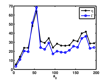
Figure 6: Dependence of the intensity boost $\eta=\max(E_{r}^{2})/\max(E_{i}^{2})$ and the pulse compression $\Gamma=(\omega_{0}\tau)^{-1}$, where $\tau$ is the FWHM width of the attosecond intensity peak in the reflected radiation, on $a_{0}$. The laser amplitude $a_{0}$ is varied between 5 and 195 in steps of 10. Other parameters are the same as in Fig. 2b.

In figure 6 the two parameters $\eta$ and $\Gamma$ are shown in dependence of $a_{0}$. Except for the variation of $a_{0}$, the parameters chosen are the same as in Figs.1c-d, 2b and 5.

First of all we notice, that for all simulations in this series with $a_{0}\gg 1$, we find $\eta\gg 1$. Thus, Eq. (1) is violated in all cases. Since we also notice $\Gamma\gg 1$ and $\Gamma\sim\eta$, we know, that the radiation is emitted in the shape of attosecond peaks with an efficiency of the order 1. This indicates, that we can describe the radiation as CSE. The perhaps most intriguing feature of Fig. 6 is the strongly pronounced peak of both curves around $a_{0}=55$. We think that because of some very special phase matching between the turning point of the electron bunch and of the electromagnetic wave, the electron bunch experiences an unusually high compression at this parameter settings. This is the case that was discussed in section III.

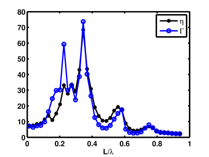
Figure 7: Dependence of the intensity boost $\eta=\max(E_{r}^{2})/\max(E_{i}^{2})$ and the pulse compression $\Gamma=(\omega_{0}\tau)^{-1}$, on the plasma scale length in units of the laser wavelength $L/\lambda$ in the lab frame. Except for the plasma scale length, parameters are the same as in Fig. 2b. The plasma ramp is again an exponential one $\propto\exp(x/L)$.

Figure 7 shows the two parameters $\eta$ and $\Gamma$ as functions of the plasma gradient scale length $L$. It is seen that both functions possess several local maxima. Further, $\eta$ and $\Gamma$ behave similar apart from one runaway value at $L=0.225\lambda$, where the FWHM peak duration is extremely short, but the intensity boost is not as high. A look at the actual field data tells us that in this case the foot of the attosecond peak is broader, consuming most of the energy. This deviation might e.g. be caused by a different, non-gaussian shape of the electron nanobunch.

The maximum of both functions lies around $L=0.33\lambda$, the parameter setting analyzed in detail before. In the limit of extremely small scale lengths $L\lesssim 0.1\lambda$, $\eta$ and $\Gamma$ become smaller, but they remain clearly bigger than one. Thus the reflection in this parameter range can still not very well be described by the ARP boundary condition. For longer scale lengths $L>0.8\lambda$, both key values approach 1, so the ARP boundary condition can be applied here. This is a possible explanation, why the BGP spectrum (2) could experimentally measured at oblique incidence Dromey2006 .

VII Conclusions

In this paper we have identified a novel mechanism of harmonics generation at overdense plasma surfaces, leading to the flattest harmonics spectrum known so far. Extremely dense and narrow peaks in the electron density, we call them nanobunches, are responsible for the radiation. The spectrum can be understood as a 1D synchrotron spectrum emitted by a relativistically moving, extremely narrow and dense electron layer. Like the CWE and ROM harmonics, the CSE harmonics are phase locked and appear in the form of attosecond pulses. In contrast to CWE and ROM, the attosecond pulses are visible immediately, therefore no energy needs to be wasted in spectral filtering and the energy efficiency of attosecond pulse generation is close to 100%.

The work has been supported by DFG Transregio SFB TR18 and Graduiertenkolleg GRK 2103.

References

- (1) A. Pukhov, Nature Physics 2, 439 (2006).
- (2) Y. Nomura, R. Horlein, P. Tzallas, B. Dromey, S. Rykovanov, Z. Major, J. Osterhoff, S. Karsch, L. Veisz, M. Zepf, D. Charalambidis, F. Krausz, and G. D. Tsakiris, Nature Physics 5, 124 (2009).
- (3) F. Quere, C. Thaury, P. Monot, S. Dobosz, P. Martin, J.-P. Geindre, and P. Audebert, Phys. Rev. Lett. 96, 125004 (2006).
- (4) R. Lichters, J. M. ter Vehn, and A. Pukhov, Phys. Plasmas 3, 3425 (1996).
- (5) B. Dromey, D. Adams, R. Horlein, Y. Nomura, S. G. Rykovanov, D. C. Carroll, P. S. Foster, S. Kar, K. Markey, P. McKenna, D. Neely, M. Geissler, G. D. Tsakiris, and M. Zepf, Nature Physics 5, 146 (2009).
- (6) A. Tarasevitch, K. Lobov, C. Wunsche, and D. von der Linde, Phys. Rev. Lett. 98, 103902 (2007).
- (7) T. Baeva, S. Gordienko, and A. Pukhov, Phys. Rev. E 74, 046404 (2006).
- (8) B. Dromey, M. Zepf, A. Gopal, K. Lancaster, M. S. Wei, K. Krushelnick, M. Tatarakis, N. Vakakis, S. Moustaizis, R. Kodama, M. Tampo, C. Stoeckl, R. Clarke, H. Habara, D. Neely, S. Karsch, and P. Norreys, Nature Physics 2, 456 (2006).
- (9) T. J. M. Boyd and R. Ondarza-Rovira, Phys. Rev. Lett. 101, 125004 (2008).
- (10) A. Bourdier, Physics of Fluids 26, 1804 (1983).
- (11) D. An der Brügge and A. Pukhov, Physics of Plasmas 14, 093104 (2007).
- (12) S. Gordienko, A. Pukhov, O. Shorokhov, and T. Baeva, Phys. Rev. Lett. 93, 115002 (2004).
- (13) J. D. Jackson, Classical Electrodynamics, J. Wiley & Sons Inc., 3rd ed. edition, 1998.
- (14) J. N. L. Connor, P. R. Curtis, and D. Farrelly, Journal of Physics A Mathematical General 17, 283 (1984).