Oscillatory and monotonic modes of longwave Marangoni convection in a thin film

Abstract

We study longwave Marangoni convection in a layer heated from below. Using the scaling $k=O(\sqrt{\rm Bi})$, where $k$ is the wavenumber and ${\rm Bi}$ is the Biot number, we derive a set of amplitude equations. Analysis of this set shows presence of monotonic and oscillatory modes of instability. Oscillatory mode has not been previously found for such direction of heating. Studies of weakly nonlinear dynamics demonstrate that stable steady and oscillatory patterns can be found near the stability threshold.

Introduction. Marangoni convection in a liquid layer with upper free boundary is a classical problem in the dynamics of thin films and in the pattern formation books ; reviews . In the pioneer theoretical paper, Pearson Pearson analyzed the linear stability of the layer with a nondeformable free surface. He considered two cases of thermal boundary conditions at the substrate: the ideal and poor heat conductivity, when either the temperature or the heat flux are specified. In the latter case he found a monotonic longwave instability mode for heating from below and zero Biot number $\rm Bi$. For ${\rm Bi}\ll 1$ the critical wavenumber $k$ is proportional to ${\rm Bi}^{1/4}$ books . Many authors extended the analysis in order to include the deformation of the free surface. Review of analytical and numerical works can be found in books . In particular, several oscillatory modes were revealed; these modes were reported only for heating from above.

In the case of heating from below, a nonlinear analysis for ideally conductive substrate was performed in Ref. VanHook : it was shown that the subcritical bifurcation occurs and instability with necessity results in film rupture. The behavior of perturbations near the stability threshold was studied in G_YV for the case of a poorly conductive substrate. Under assumption of large gravity, and, hence, small surface deflection, the amplitude equation was derived and the subcritical bifurcation was found.

In this paper we demonstrate the existence of a new oscillatory mode of longwave instability for the film heated from below. Using the scaling $k=O(\sqrt{\rm Bi})$, which was first suggested in Ref. Alla-05 , we derive a set of amplitude equations. Linear stability analysis gives both the monotonic and the oscillatory modes. Pattern selection near the stability threshold clearly demonstrates that instability does not necessarily lead to rupture and that both steady and oscillatory regimes can be found experimentally within certain domains of parameters.

Problem formulation. We consider a three-dimensional thin liquid film of the unperturbed height $H_{0}$ on a planar horizontal substrate heated from below. The heat conductivity of the solid is assumed small in comparison with the one of the liquid, thus the constant vertical temperature gradient $-A$ is prescribed at the substrate. (The Cartesian reference frame is chosen such that the $x$ and $y$ axes are in the substrate plane and the $z$ axis is normal to the substrate.)

The dimensionless boundary-value problem governing the fluid dynamics reads:

$$\frac{1}{P}\left({\bf v}_{t}+{\bf v}\cdot\nabla{\bf v}\right) = -{\bf\nabla}p+\nabla^{2}{\bf v}-G{\bf e}_{z},$$ (1a)

$$T_{t}+{\bf v}\cdot\nabla T = \nabla^{2}T,\ \nabla\cdot{\bf v}=0,$$ (1b)

$${\bf v} = 0,\ T_{z}=-1\ {\rm at}\ z=0,$$ (2a)

$${\bf\Sigma}\cdot{\bf n} = \left(p-{\rm Ca}K\right){\bf n}-M\nabla_{\tau}\left(T|_{z=h}\right),\ \nabla_{n}T=-{\rm Bi}\;T,$$

$$h_{t} = w-{\bf v}\cdot{\bf\nabla}h\ {\rm at}\ z=h(x,y,t).$$ (2b)

Here, ${\bf v}=({\bf u},w)$ is the fluid velocity (where ${\bf u}$ is the velocity in the substrate plane and $w$ is the $z$-component), $T$ is the temperature, $p$ is the pressure in the liquid, $\bf\Sigma$ is the viscous stress tensor, $h$ is the dimensionless height of the film, ${\bf e}_{z}$ is the unit vector directed along the $z$ axis, ${\bf n}$ and $\bf\tau$ are the normal and tangent unit vectors to the free surface, respectively, $K$ is the mean curvature of the free surface. The dimensionless parameters entering the above set of equations are the capillary number, the Marangoni number, the Galileo number, the Biot number, and the Prandtl number:

$${\rm Ca}=\frac{\sigma H_{0}}{\eta\chi},\ M=-\frac{\sigma_{T}AH_{0}^{2}}{\eta\chi},\ G=\frac{gH_{0}^{3}}{\nu\chi},\ {\rm Bi}=\frac{qH_{0}}{\kappa},$$

and $P=\nu/\chi$. Here $\sigma$ is the surface tension, $\sigma_{T}\equiv d\sigma/dT$, $g$ is the acceleration of gravity, $q$ is the heat transfer rate, $\kappa$ is the thermal conductivity, $\chi$ is the thermal diffusivity, $\nu$ and $\eta$ are the kinematic and dynamics viscosity of liquid, respectively.

Below we study evolution of a large-scale convection using the set of Eqs. (1) and (2).

Amplitude equations. We rescale the coordinates and the time as follows:

$$X=\epsilon x,\ Y=\epsilon y,\ \tau=\epsilon^{2}t,$$ (3)

where $\epsilon\ll 1$ is the ratio of $H_{0}$ to a typical horizontal lengthscale. The temperature field is represented as $T=-z+{\rm Bi}^{-1}+\theta(X,Y,\tau)+O(\epsilon^{2})$.

We assume large values of ${\rm Ca}$ and small values of $\rm Bi$,

$${\rm Ca}=\epsilon^{-2}C,\ {\rm Bi}=\epsilon^{2}\beta.$$ (4)

Thus we deal with the intermediate asymptotics between the conventional longwave mode, ${\rm Bi}=O\left(\epsilon^{4}\right)$, G_YV and the case of finite $\rm Bi$ Pearson . These cases correspond to $\beta=0$ and $\beta\to\infty$, respectively.

Substituting the rescaled fields into Eqs. (1) and (2) and applying the conventional technique of the lubrication approximation (see reviews ), we arrive at

$$h_{\tau} = {\bf\nabla}\cdot\left[\frac{h^{3}}{3}{\bf\nabla}\Pi+\frac{Mh^{2}}{2}{\bf\nabla}\left(\theta-h\right)\right]\equiv{\bf\nabla\cdot j},$$ (5)

$$h\theta_{\tau} = {\bf\nabla}\cdot\left(h{\bf\nabla}\theta\right)-\frac{1}{2}(\nabla h)^{2}-\beta(\theta-h)+{\bf j}\cdot{\bf\nabla}(\theta-h)$$ (6)

$$+{\bf\nabla}\cdot\left[\frac{h^{4}}{8}{\bf\nabla}\Pi+\frac{Mh^{3}}{6}{\bf\nabla}(\theta-h)\right].$$

Here $\Pi=Gh-C\nabla^{2}h$ and $\nabla$ is a two-dimensional gradient with respect to $X$ and $Y$.

Equations (5) and (6) form a closed set of the amplitude equations governing the nonlinear interaction of two well-known longwave modes: the Pearson’s mode ($h=1$) Pearson and the surface deformation-induced mode. (Note that the latter mode with $\theta=const$ emerges only in the case of the conductive substrate VanHook .) Conductive state obviously corresponds to $h=\theta=1$.

Linear stability analysis. Substituting the perturbed fields $h=1+\xi$ and $\theta=1+\Theta$ into Eqs. (5) and (6), linearizing the equations for perturbations about the equilibrium, and representing the perturbation fields proportional to $\exp\left(\lambda\tau+ikX\right)$, one arrives at

$$\lambda^{2}+\lambda\left[\beta+k^{2}\left(1+\frac{\tilde{G}-M}{3}\right)\right]$$

$$+\frac{k^{2}}{3}\left(\beta+k^{2}\right)\tilde{G}-\frac{Mk^{4}}{2}\left(1+\frac{\tilde{G}}{72}\right)=0,$$ (7)

where $\tilde{G}\equiv G+Ck^{2}$. Equation (7) possesses both real (monotonic instability) and complex (oscillatory instability) solutions.

For the monotonic mode $\lambda=0$ at the stability border, thus the marginal stability curve is given by

$$M_{m}=\frac{48\left(\beta+k^{2}\right)\tilde{G}}{k^{2}\left(72+\tilde{G}\right)}.$$ (8)

These marginal curves have a minimum at the finite values of $k$ only if

$$\beta C<72,$$ (9)

otherwise the minimal value, $M_{c}^{(m)}$, is achieved in the limit $k\to\infty$, i.e. the longwave mode is not critical. Hereafter we assume that the inequality (9) holds; since the limit $C=0$ is well studied , for all computations we set $C=1$ without loss of generality . The critical wavenumber materializing the minimum of the marginal stability curve, Eq. (8), is

$$\left(k_{c}^{(m)}\right)^{2}=\frac{\beta CG+\sqrt{72\beta CG\left(G+72-\beta C\right)}}{C\left(72-\beta C\right)}.$$

Figure 1: (a): Marginal stability curves $M_{*}(k)$ for $G=10$: solid lines correspond to the monotonic mode, dashed ones – to the oscillatory mode; $\beta=1,\,10,\,40$ for lines 1, 2, and 3, respectively. (b): The domain of oscillatory instability. The dashed vertical line marks the boundary of the longwave instability, Eq. (9).

For the oscillatory mode the marginal stability curve is determined by the expression

$$M_{o}=3+\tilde{G}+\frac{3\beta}{k^{2}}.$$ (10)

The imaginary part of the growth rate for neutral perturbations is

$$\lambda_{i}\equiv{\rm Im}(\lambda)=\frac{k^{2}}{12}\sqrt{(72+\tilde{G})\left(M_{m}-M_{o}\right)},$$ (11)

i.e. the oscillatory mode is present only at $M_{o}(k)<M_{m}(k)$.

Minimization of the Marangoni number with respect to $k$ gives

$$M_{c}^{(o)}=3+G+2\sqrt{3\beta C},\ k_{c}^{(o)}=\left(\frac{3\beta}{C}\right)^{1/4}.$$ (12)

Examples of the marginal stability curves for these modes are shown in Fig. 1(a). Domains of monotonic and oscillatory instability are demonstrated in Fig. 1(b). It is clear that the oscillatory mode is critical for $\beta C>17.4$ and $G<17.2$. Take, for instance, a layer of water of thickness $H_{0}=10^{-3}{\rm cm}$. Then $G\approx 0.1$, ${\rm Ca}\approx 10^{4}$ and $\rm Bi$ has to be approximately $10^{-3}$ in order to provide the required value of $\beta C$; this value seems achievable in experiments.

Equations (10)-(12) indicate why the oscillatory mode has not been found earlier. As we have emphasized above, all previous studies deal with either $\tilde{G}\gg 1$ Pearson , or $\beta=0$ G_YV , or $C=0$ Alla-05 . In these cases the oscillatory mode does not exist.

Weakly nonlinear analysis. Monotonic mode. Here we study the nonlinear dynamics of perturbations at small supercriticality, $M-M_{c}^{(m)}\approx 0$, see Ref. Hoyle-book . To this end, we represent the primary part of the small perturbation of $h$ in the form:

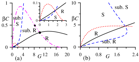
Figure 2: (Color online). Pattern selection for the monotonic mode. (a) and (b) – the domains of stability for Rolls (marked with “R”) and Squares (“S”) on the square lattice. Solid (dashed) lines separate between supercritical and subcritical branching for Rolls (Squares). The latter domains are marked by “sub. R” (“sub. S”). Dotted lines separate domains of stability for Rolls and Squares. Dashed-dotted line in panel (a) is the locus of points $N=0$; in the vicinity of this curve Eq. (17) holds. Diamond (circle) shows the threshold value $G_{1}$ ($G_{2}$) for pattern selection on the hexagonal lattice.

$$\xi=\sum_{j=1}^{n}A_{j}\exp\left(i{\bf k}_{j}\cdot{\bf R}\right)+c.c.$$ (13)

where $c.c.$ denotes complex conjugate terms and $k_{j}=k_{c}^{(m)}$. (The primary part of $\Theta$ is expressed in terms of $\xi$.) The amplitudes $A_{j}$ are functions of a slow time. For square ($n=2$) and hexagonal ($n=3$) lattices, the wavevectors are

$${\bf k}_{1} = k_{c}(1,0),\ {\bf k}_{2}=k_{c}(0,1)$$ (14)

$${\rm and}\ {\bf k}_{1} = k_{c}(1,0),\ {\bf k}_{2,3}=\frac{1}{2}k_{c}(-1,\pm\sqrt{3}),$$ (15)

respectively.

For square lattice, the amplitude equations read

$$\dot{A}_{j} = \left(\gamma-K_{0}|A_{j}|^{2}-K_{1}S_{A}\right)A_{j},\ j=1,2,$$ (16)

where $S_{A}=\sum_{1}^{n}|A_{l}|^{2}$. Here the dot denotes the derivatives with respect to the slow time, and $\gamma\sim M-M_{c}^{(m)}$ is the real growth rate. The Landau constants, $K_{0}$ and $K_{1}$ are real; they are cumbersome and thus are not presented here. Results of the numerical calculations are shown in Fig. 2. One can readily see that supercritical branching occurs only in two domains of parameters. These domains are situated either at rather small values of $\beta C$, Fig. 2(a), or at sufficiently small $G$, Fig. 2(b). In the former case Rolls are selected everywhere except for a very small region shown in the inset. In the latter case Squares are selected everywhere excluding the small region where Rolls are stable.

For hexagonal lattice, the resonant quadratic interaction results in the following amplitude equation:

$$\dot{A}_{1}=\gamma A_{1}-NA_{2}^{*}A_{3}^{*}-\left(K_{0}|A_{1}|^{2}+K_{1}S_{A}\right)A_{1},$$ (17)

and a similar equations for $A_{2,3}$. (Hereafter the asterisk denotes the complex-conjugate terms.) Generally speaking, the quadratic term prevails over cubic ones, which leads to subcritical excitation of the hexagonal patterns through a transcritical bifurcation Hoyle-book . However, $N=0$ at the dashed-dotted line shown in Fig. 2(a) and in the vicinity of this line Eq. (17) becomes appropriate.

Among the variety of possible patterns Hoyle-book , three are important. They are Rolls with $A_{1}\neq 0,\,A_{2}=A_{3}=0$ and two types of Hexagons with $A_{1}=A_{2}=A_{3}\equiv A$: $H^{+}$ for $A>0$ and $H^{-}$ in the opposite case. In the former case the flow is upward in the center of the convective cell, whereas in the latter case it is downward.

Pattern selection on a hexagonal lattice is shown in Fig. 2(a). At $G<G_{1}\approx 8.20$ there are no stable solutions; the subcritical bifurcation occurs for Rolls and one branch of Hexagons (either $H^{-}$ below or $H^{+}$ above the dashed-dotted line). At $G_{1}<G<G_{2}=10$ Rolls are still subcritical and unstable; stable Hexagons emerge only within the finite interval of supercriticality. Finally, at $G>G_{2}$, $H^{-}(H^{+})$ is stable within the interval of supercriticality, whereas Rolls become stable when $M-M_{c}^{(m)}$ increases.

To finalize the discussion of steady patterns, we briefly discuss the competition of patterns on the square and hexagonal lattices. It is clear that at the finite values of $N$, Hexagons emerge subcritically and no stable patterns can be found near the stability threshold. Therefore, weakly nonlinear analysis provides stable patterns only near the dashed-dotted curve shown in Fig. 2(a), where the competition between Hexagons and Rolls occurs.

Weakly nonlinear analysis. Oscillatory mode. For the oscillatory mode the solution is presented in the form

$$\xi=\sum_{j=1}^{n}\left(A_{j}e^{i{\bf k}_{j}\cdot{\bf R}}+B_{j}e^{-i{\bf k}_{j}\cdot{\bf R}}\right)e^{i\lambda_{i}\tau}+c.c.$$ (18)

Note that the pair $(A_{j},B_{j})$ corresponds to counter-propagating waves, which must be taken into account separately. The wavevectors for the square and hexagonal lattices are given by Eqs. (14) and (15), respectively.

For square lattice, the equation governing the dynamics of the amplitudes $A_{j}$ reads:

$$\dot{A}_{j} = \left[\gamma-K_{0}|A_{j}|^{2}-K_{1}|B_{j}|^{2}-K_{2}\left(S_{A}+S_{B}\right)\right]A_{j}$$ (19)

$$-K_{4}B_{j}^{*}S_{AB},\ j=1,2,$$

where $S_{B}=\sum_{1}^{n}|B_{l}|^{2}$, $S_{AB}=\sum_{1}^{n}A_{l}B_{l}$. A similar pair of equations for $B_{j}$ is obtained from Eqs. (19) by replacement $A_{j}\leftrightarrow B_{j}$. The Landau coefficients $K_{l}$ ($l=0,1,2,4$) as well as the growth rate $\gamma$ are now complex-valued.

Equations (19) were studied in details in Ref. Silber-Knobloch . Using the results of that paper, we found that Traveling Rolls (TR), $A_{1}\neq 0,\,A_{2}=B_{1,2}=0$ can branch either supercritically or subcritically [see Fig. 3(a)], whereas the remaining patterns emerge through the direct Hopf bifurcation; TR are selected in the domain of supercritical excitation. Alternating Rolls are stable within the small area marked by “AR”; here depending on the initial condition the system either approaches AR or demonstrates the infinite growth of TR.

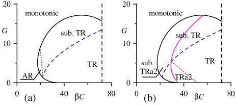
Figure 3: (Color online). Pattern selection for the oscillatory convection. (a) – square lattice: Domains of stability for TR (below the dashed line) and AR (to the left of the dotted line). Above the dashed line TR bifurcate subcritically. (b) – hexagonal lattice: Domains of stability for TR (below the dashed line and to the right of the dotted line) and TRa2 (between the dotted and the solid line) are marked by “TR” and “TRa2”, respectively. Above the dashed line TR bifurcate subcritically, to the left of the solid line TRa2 are subcritical.

For hexagonal lattice, the amplitude equation governing the dynamics of the complex amplitudes $A_{j}$ reads:

$$\dot{A}_{j} = \left[\gamma-K_{0}|A_{j}|^{2}-K_{1}|B_{j}|^{2}-K_{2}S_{A}-K_{3}S_{B}\right]A_{j}$$ (20)

$$-K_{4}B_{j}^{*}S_{AB},\ j=1,2,3.$$

Three similar equations are obtained from Eqs. (20) by a replacement $A_{j}\leftrightarrow B_{j}$.

Analysis of the Hopf bifurcation for the above set of equations was performed in Ref. Roberts , where eleven limit cycles were found and studied. Based on that paper, the results on pattern selection are presented in Fig. 3(b). The dashed line again separates direct and inverse Hopf bifurcations for TR, it is obviously the same as in the panel (a). However, for the hexagonal lattice, there appears a competition between TR and Traveling Rectangles 2 (TRa2, $A_{1}=B_{3}\neq 0$, whereas all other amplitudes vanish). The latter pattern is stable in the domain marked by “TRa2”. The entire domain of supercritical bifurcation becomes smaller because TRa2 can bifurcate either supercritically or subcritically.

Studying the competition between patterns on hexagonal and square lattices, we found that the stability boundaries for both TR and TRa2 are the same as shown in Fig. 3(b), whereas stability domain for AR nearly disappears.

Conclusions. We studied the longwave Marangoni convection in a liquid layer heated from below; the heat flux at the substrate is specified. In such setup, an interaction of two well-known monotonic modes of longwave instability, the Pearson’s mode and the surface deformation-induced mode, can result in the emergence of a longwave oscillatory mode. However, the oscillatory mode has not been detected in spite of extensive numerical, analytical, and experimental studies books since the publication of Pearson’s paper. We succeed in such analysis and point out the domain of parameters where the oscillatory mode exists, which can be reached in experiments.

Moreover, we point out the domains of parameters where the convection emerges supercritically and hence either stationary or oscillatory terminal state with distorted surface is stable. This result is also very unusual, since only subcritical branching was found in the previous studies VanHook ; G_YV .

Acknowledgments. We are grateful to A. A. Nepomnyashchy and A. Oron for the fruitful discussions. S.S. and A.A. are partially supported by joint grants of the Israel Ministry of Sciences (Grant 3-5799) and Russian Foundation for Basic Research (Grant 09-01-92472). M.K. acknowledges the support of WKU Faculty Scholarship Council via grants 10-7016 and 10-7054.

References

- (1) P. Colinet, J.C. Legros, and M.G. Velarde, Nonlinear Dynamics of Surface-Tension-Driven Instabilities (Wiley-VCH, Berlin, 2001); A. A. Nepomnyashchy, M.G. Velarde, and P. Colinet, Interfacial Phenomena and Convection (Chapman and Hall/CRC Press, London, 2001); R. V. Birikh et al., Liquid Interfacial Systems. Oscillations and Instability (Marsel Dekker, New York, Basel, 2003).
- (2) A. Oron, S. H. Davis, and S. G. Bankoff, Rev. Mod. Phys. 69, 931 (1997); R. V. Craster, O. K. Matar, Rev. Mod. Phys. 81, 1131 (2009).
- (3) J. R. A. Pearson, J. Fluid Mech. 4, 489 (1958).
- (4) S. J. VanHook et al., J. Fluid Mech. 345, 45 (1997).
- (5) P. L. Garcia-Ybarra, J. L. Castillo, and M. G. Velarde, Phys. Fluids 30, 2655 (1987); A. Oron and P. Rosenau, Phys. Rev. A 39, 2063 (1989).
- (6) A. Podolny, A. Oron, and A. A. Nepomnyashchy, Phys. Fluids 17, 104104 (2005).
- (7) R. B. Hoyle, Pattern Formation: An Introduction to Methods Cambridge University Press, Cambridge, 2006.
- (8) M. Silber, E. Knobloch, Nonlinearity 4, 1063 (1991).
- (9) M. Roberts, J.W. Swift, and D.H. Wagner, Multiparameter Bifurcation Theory, eds. M. Golubitsky and J. Guckenheimer, Contemp. Math. 56, 283 (1986).