Statistical Estimation of Quantum Tomography Protocols Quality
Abstract
A novel operational method for estimating the efficiency of quantum state tomography protocols is suggested. It is based on a-priori estimation of the quality of an arbitrary protocol by means of universal asymptotic fidelity distribution and condition number, which takes minimal value for better protocol. We prove the adequacy of the method both with numerical modeling and through the experimental realization of several practically important protocols of quantum state tomography.
pacs:
42.50-p, 42.50.Dv, 03.67.apacs:
42.50.-p, 42.50.Dv, 03.67.-aIntroduction. Quantum states and processes being a fundamental tool for basic research, also become a resource for developing quantum technologies physrep : this
demands for their characterization. At present
quantum state/process tomography serves as a standard instrument
tomo for characterizing quality of preparation and
transformation of quantum states. Basically it includes a given set of unitary
transformations over the state to be reconstructed, then
the transformed state is measured and finally some computational
procedure applied to the measuring outcomes completes the state
reconstruction. The result is a state vector or a density matrix. In
order to compare different schemes the achieved result can
eventually be checked by calculating some distance measure, like
fidelity, that shows the quality of preparation/reconstruction of
the quantum state.
It is worth to mention that in real experiments the accuracy of the reconstruction depends on two types of uncertainties: statistical and instrumental ones.
If the total number of measurement outcomes (sample size or
statistics) is large enough, the instrumental uncertainties dominate
over fundamental statistical fluctuations caused by probabilistic
nature of quantum phenomena PRA_qutrit . Practically the
required statistics, allowing to exclude statistical
fluctuations, depends on the tomographic protocol itself and the total accumulating time needed for taking data. From this point of view it is of the utmost interest to point out simple and universal algorithms for the estimation of the chosen protocol on design stage before doing experiments as well as the sample size for desirable quality of the state reconstruction.
In this letter we propose a universal method for estimating the quality of any tomographic protocol based on discrete degrees of freedom and test it with well-known reconstruction protocols of polarization states of qubit pairs. Since it represents a paradigmatic example, here we restrict ourselves to polarization degrees of freedom only. Manipulations
with polarization qubits, qutrits and ququarts have been discussed widely in context of quantum state reconstruction and its optimization kwiat ; PRA_qutrit ; PRA_ququart ; D'Ariano ; Rehacek ; Kurtsiefer ; Burgh ; pas ; nos .
Theory and numerical simulation An arbitrary -dimensional quantum state is completely described by a state vector in a -dimensional Hilbert space when it is a pure state, or by a density matrix for a mixed one. To measure the quantum state one needs to perform a set of projective measurements. According to Bohr’s complementarity principle, it is impossible to measure all projections simultaneously, operating with a single representative of the quantum state only. So, first of all, one needs to generate a set of copies of the state D'Ariano . Then for each measurement outcome rates can be evaluated from amplitudes of a quantum process
| (1) |
The amplitudes cannot be measured directly, but they are linearly related to the state vector root-est . For an arbitrary protocol based on measurements the process amplitudes can be represented as:
| (2) |
being the state vector and a row of the so called instrumental matrix , which describes the entire set of mutually-complementary measurements. The normalization condition for the protocol bounds the total expected number of events and the acquisition time : . We define the row of the measurement matrix for a tomographic protocol as the direct product , its size being and we assume . By using the matrix , the protocol can be compactly written in the matrix form:
| (3) |
Here is the density matrix, given in the form of a column (second column lies below the first, etc.). The vector of length records the total number of registered outcomes. The algorithm for solving equation (3) is based on the so called singular value decomposition (svd) svd . Svd serves as a base for solving inverse problem by means of pseudo-inverse (PI) or Moore-Penrose inverse Penrose . In summary, matrix can be decomposed as:
| (4) |
where () and () are unitary matrices and () is a diagonal, non-negative matrix, whose diagonal elements are ”singular values”. Then (3) transforms to a simple diagonal form:
| (5) |
with a new variable unitary related to as and a new column unitary related to the vector as . We use this algorithm as a starting approximation for maximal likelihood state reconstruction. By defining as the number of non-zero singular values of we formulate two important conditions of any tomography protocol, namely its completeness and adequacy future . The protocol is supposed to be informationally complete if the number of tomographically complementary projection measurements is equal to the number of parameters to be estimated; mathematically completeness means . Adequacy means that the statistical data directly correspond to the physical density matrix (which has to be normalized, Hermitian and positive). However, generally for mixed state it can be tested only if the protocol consists of redundant measurements, i.e. .
PI provides with zero approximation for estimated parameters of quantum states. Optimization of these parameters can be done following the approach developed in PRA_qutrit in the frame of maximal likelihood method. It is worth to stress that the reconstructed state vector extracted from the likelihood equation associates with finite statistics of the registered outcomes of an experiment and therefore takes random
values. The difference between the reconstructed state vector and
its exact value is caused by statistical fluctuations
instrumental . The complete information matrix introduced in
PRA_qutrit ; root-est allows analyzing arbitrary functions on
fluctuating parameters of quantum states. One very relevant
function in the context of quantum state/process estimation is
fidelity where and being
the exact and the reconstructed density matrices correspondingly,
tending to identity for complete protocols with an unlimited
increase of a sample size.
Basically the problem of the state reconstruction splits into two scenarios. The first one relates to
the case when the reconstructed state is known in advance (like in
quantum cryptography). Then statistical comparison between exact
theoretical state and reconstructed one allows one either to reveal
the source of instrumental uncertainties or to be sure that such
uncertainties are small enough in comparison with statistical
fluctuations. The second case occurs when the reconstructed state is
unknown. Then using the approach developed below one should
calculate the statistical distribution of fidelity between unknown
exact state and reconstructed (by means of maximal likelihood
method) one. Fidelity will be either inside the uncertainty boundary
for small statistics or outside for large statistics (when
instrumental uncertainties prevail). In this case it is convenient
to analyze the so called fidelity loss . When the
reconstruction accuracy is determined by a finite number of
representatives of the quantum state, fidelity loss is a random
variable whose asymptotic distribution can be represented as
Bogdanov09 :
| (6) |
where are independent and normally distributed random variables with zero mean values and unit dispersion, , for pure states, for mixed states. The coefficients can be extracted from the complete information matrix Bogdanov09 . Distribution (6) is a natural generalization of the - distribution for which all . As it follows from (6) the average value of fidelity loss is:
| (7) |
PI implies introduction of so called condition number , which is defined as the ratio between the minimal nonzero singular eigenvalue of and maximal one
| (8) |
determines the stability of the linear system (3)
and therefore can be used as a practical quantifier for estimating
efficiency of the protocol: the lower the better the protocol.
If at least one of singular eigenvalues is close to
zero then the protocol
becomes incomplete and . The optimal value of would be unity that means uniform distribution of singular values future .
The present approach allows to analyze arbitrary protocols of statistical reconstruction of quantum states.
As an example we have selected three popular protocols. The first,
suggested in kwiat and dubbed J16 Burgh , is suited for
reconstructing 4-dimensional polarization states, as photon pairs
degenerate in frequency generated in the process of spontaneous
parametric down-conversion (SPDC). In this protocol the projective
measurements upon some components of Stokes vector are performed for
each qubit in pair individually, so the 16 two-qubit measurements
are , , , , , , , , , ,
, , , , , where , , , ,
denotes horizontal, vertical, right and left circular and
diagonal polarizations respectively. Here, for example, the
measurement setting means measuring horizontal polarization on
the first qubit and right circular polarization on the second qubit
in pair. In our formalism the protocol can be represented by an
instrumental matrix with 16 rows .
In the case of independent measurement of two qubits the projective measurements can be chosen arbitrarily. In Rehacek measured qubits were projected on the states possessing tetrahedral
symmetry (R4). There are several works showing that due to
the high symmetry such protocol provides a better quality of
reconstruction Kurtsiefer ; Burgh . Let us stress that since
the adequacy of both R16 and J16 can not be
tested.
We also consider a protocol where the whole single-beam two-qubit state is subjected to linear transformations using two retardation plates
PRA_ququart (B144). The total number of
projective measurements is redundant and equals to 144, so the
corresponding instrumental matrix has 144 rows and protocol admits
adequacy testing, being .
For these protocols we calculate condition numbers which take the following values: , , B144opt . Thus, we expect that the symmetrical protocol R16 provides with better state reconstruction
quality Burgh . We have checked this statement with numerical
simulations of each protocol applied to different two-qubit states
depending on the sample size.
As an example, let us consider the numerical reconstruction of the Bell
state .
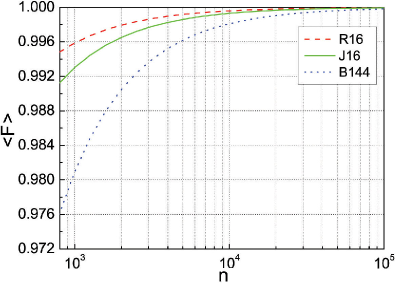
Fig. 1 shows average fidelities, calculated according to (7) as functions of sample size for each protocol.
It turns out that the difference between curves disappears at sufficiently large sample size () instrumental ,
but for the same quality of state reconstruction the correct choice of protocol allows using a smaller set of statistical data,
i.e. finally reduces total acquisition time. Fig. 1 shows that protocols are ranged in accuracy as following: R16, J16, and B144
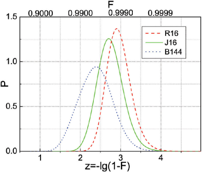
in complete agreement with the range given by condition number K. Fig.2 presents accuracy distributions calculated according to (6) for the sample size .
For better visualization we transformed the abscissa scale into particular common logarithmic one as .
Corresponding integers indicate the number of nines in fidelity recording. The density distribution for the R16 protocol
is narrower than the one for J16 and B144 and localizes in the region of lower losses or higher fidelities.
The distribution for B144 is broader and lower in comparison with R16 and J16.
Obviously, the narrower distribution of fidelity indicates a better reconstruction quality in the sense that
the reconstruction procedure returns a better-defined state. Thus, Fig.2
confirms our expectation based on estimation of condition number : R16 achieves the best results.


Experiment. We prepared a family of two-photon polarization states which can be easily converted into both entangled (in polarization) and factorized states
| (9) |
with real amplitudes and . The set-up is schematically depicted in Fig. 3.

A cw argon laser beam at pumps, after having selected by a Glan-Thompson prism (GP) its horizontal polarization, two type-I BBO crystals (1 mm) positioned with the planes that contain optical axes orthogonal to each other. The halfwave plate placed in front of crystals () rotates the polarization of the pump by the angle which controls real amplitudes and in (9). The crystals are cut for collinear frequency non-degenerate phase-matching around central wavelength 702nm. The relative phase shift in (9) is controlled by tilting quartz plates QP. If we prepare the state , if and then the state transforms to .
To maintain stable phase-matching conditions, BBO crystals and QP
are placed in a closed box heated at fixed temperature. The lens
couples SPDC light into the monochromator M (with 1 nm resolution),
set to transmit ”idler” photons at 710nm. The conjugate ”signal”
wavelength 694 nm is selected automatically by means of coincidence
scheme. Zero-order wave plates () are used in
both J16 and R16 for arranging the projective measurement
set. In B144 these plates were removed and additional
achromatic quartz plates WP1,2 (0.9183 mm, 0.9167 mm)
established the necessary measurement set at given wavelengths
PRA_ququart .
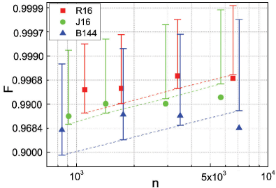
For protocols described above the statistical reconstruction of prepared states (9) has been performed at given sample sizes. As an example, Fig.(4) shows calculated
widths of fidelity distributions at 1%- and 99%- quantiles for the
three protocols (see Fig.2) as well as the
experimentally reconstructed values for the specific state
.

The approach described above provides the ideal accuracy level for
quantum state reconstruction. It means that fluctuations of the
estimated quantum states certainly cannot lead to uncertainties
smaller than this limit. Presence of instrumental uncertainties
makes this level to be exceeded. Indeed, Fig.4 shows that,
beginning from some sample size, the experimental value of fidelity
falls out the theoretical uncertainty boundary shown as dotted lines
(corresponding to 1% significance level which characterizes a given
protocol). This happens since instrumental uncertainties prevail
over the statistical ones and indicates that either state
preparation stage or measurement procedure were not performed
accurately enough. Incidentally, the absence of uncertainty bars for
data in Fig.4 derives from running once the corresponding protocol.
Repeated measurements would provoke appearance of a statistical
uncertainty, however respective theoretical uncertainty levels
should be re-scaled.
Definitely comparison between reconstructed states and fundamental
statistical fluctuations can serve to achieve precise adjustment of
the set-up, detection of the unapproved incursion into communication
channel, etc.
Conclusion. We have proposed and tested, both by numerical calculation and experimental realization, a new estimation scenario of tomographic protocols. Our results demonstrate the potentialities of this method for a widespread application to experiments on fundamental quantum optics and quantum technologies. Indeed, it can provide in advance, based on condition number , indications on the uncertainty that can be reached for a certain set-up by a tomographic scheme, providing experimentalist with a tool for choosing the best protocol based on available experimental resources (retardant plates, polarization filters, etc.) and limited available time for data acquisition. Also we would like to stress that the developed method is quite general and that it can be applied to any sort of quantum states and measurement sets future .
Acknowledgments. This work was supported in part by Russian Foundation of Basic Research (projects 08-02-00741a, 10-02-00204a, 08-07-00481a), Leading Russian Scientific Schools (project 65179.2010.2), MIUR (PRIN 2007FYETBY) and NATO (CBP.NR.NRCL.983251).
References
- (1) M. Genovese, Phys. Rep. 413, 319 (2005).
- (2) A.I. Lvovsky et al, Phys. Rev. Lett. 87, 050402 (2001); A. Zavatta et al., Phys. Rev. A 70, 053821 (2004); A. Allevi et al., Phys. Rev. A 80 (2009) 022114; G. Zambra et al., Phys. Rev. Lett. 95, 063602 (2005).
- (3) Yu.Bogdanov et al., Phys. Rev. A 70, 042303 (2004).
- (4) D.F.V.James et al.. Phys. Rev. A 64, 052312 (2001).
- (5) Yu.Bogdanov et al., Phys. Rev. A. 73, 063810 (2006).
- (6) G.M.D Ariano, P.Mataloni and M.F.Sacchi, Phys. Rev. A. 71, 062337 (2005).
- (7) J.Rehacek, B.-G. Englert and D.Kaszlikowski, Phys. Rev. A 64, 052312 (2001).
- (8) A.Ling, et al. Phys. Rev. A 74, 022309 (2006); A.Ling, et al., quant-ph.0807.0991.
- (9) N.D.de Burgh, et al., Phys. Rev. A 78, 052122 (2008).
- (10) M.Asorey et al., Physical Review A 77, 042115 (2008).
- (11) G.Brida et al., quant-ph.0907.4117.
- (12) Yu.I.Bogdanov, quant-ph.0312042.
- (13) R.Kress, Numerical Analysis. Springer, Verlag New York, Inc. (1998).
- (14) R.Penrose, Proc. of Cambridge Philosophical Soc. 51, 406 (1955).
- (15) M.Genovese et al., to be published.
- (16) It holds if one can neglect instrumental uncertainties.
- (17) Yu.I.Bogdanov, JETP, 108, 928 (2009).
- (18) Condition number for B144 can be optimized by chosing appropriate plates.