On a class of scaling FRW cosmological models

Abstract

We study Friedmann-Robertson-Walker cosmological models with matter content composed of two perfect fluids $\rho_{1}$ and $\rho_{2}$, with barotropic pressure densities $p_{1}/\rho_{1}=\omega_{1}=const$ and $p_{2}/\rho_{2}=\omega_{2}=const$, where one of the energy densities is given by $\rho_{1}=C_{1}a^{\alpha}+C_{2}a^{\beta}$, with $C_{1}$, $C_{2}$, $\alpha$ and $\beta$ taking constant values. We solve the field equations by using the conservation equation without breaking it into two interacting parts with the help of a coupling interacting term $Q$. Nevertheless, with the found solution may be associated an interacting term $Q$, and then a number of cosmological interacting models studied in the literature correspond to particular cases of our cosmological model. Specifically those models having constant coupling parameters $\tilde{\alpha}$, $\tilde{\beta}$ and interacting terms given by $Q=\tilde{\alpha}H\rho_{{}_{DM}}$, $Q=\tilde{\alpha}H\rho_{{}_{DE}}$, $Q=\tilde{\alpha}H(\rho_{{}_{DM}}+\rho_{{}_{DE}})$ and $Q=\tilde{\alpha}H\rho_{{}_{DM}}+\tilde{\beta}H\rho_{{}_{DE}}$, where $\rho_{{}_{DM}}$ and $\rho_{{}_{DE}}$ are the energy densities of dark matter and dark energy respectively. The studied set of solutions contains a class of cosmological models presenting a scaling behavior at early and at late times. On the other hand the two-fluid cosmological models considered in this paper also permit a three fluid interpretation which is also discussed. In this reinterpretation, for flat Friedmann-Robertson-Walker cosmologies, the requirement of positivity of energy densities of the dark matter and dark energy components allows the state parameter of dark energy to be in the range $-1.37\lesssim\omega_{{}_{DE}}<-1/3$.

Keywords: dark energy theory, dark matter theory

I Introduction

Recent observational data indicate that our Universe is undergoing accelerated expansion. The standard modern cosmological models consider the total energy density of the Universe to be dominated today by the densities of two components: dark matter (which has an attractive gravitational effect like usual matter), and dark energy (a kind of vacuum energy with a negative pressure), which drives the accelerated expansion Lima . Even more, observational data seem to indicate that the Universe today may be dominated by an exotic kind of dark energy which has a very strong negative pressure, denominated phantom fluid since it violates all energy conditions Caldwell . The real nature of the dark sector remains unknown.

Most considered dark energy models present an accelerated expansion due to the presence of a quintessence (described by a canonical scalar field), or a phantom field (described by a scalar field with a negative kinetic term), among others. It appears in this kind of models that the energy density of dark energy is almost equivalent to that of the matter in the current or in recent times although they scale independently during all the cosmic evolution. This situation is referred to as the “coincidence problem”. To solve the coincidence problem many attempts have been done. Of special interest are interacting cosmological models since they may alleviate or even solve the coincidence problem Zimdahl . We shall refer to this type of cosmological models below in this section.

In the framework of General Relativity, for modeling the present state of the Universe, usually the cosmological models consider two cosmic fluids as sources for the Einstein field equations: one fluid for the dark matter sector, where is included the standard visible matter, and another cosmic fluid for the dark energy sector. Usually the dark matter is described as a pressureless ideal fluid, while the dark energy may be described by a cosmological constant, or perfect fluid or scalar fields Sahni .

The consideration of two fluids in Einstein field equations leads to

$$R_{\mu\nu}-\frac{1}{2}Rg_{\mu\nu}=\kappa\left(T^{1}_{\mu\nu}+T^{2}_{\mu\nu}\right),$$ (1)

where $\kappa=8\pi G$, and $T^{1}_{\mu\nu}$ and $T^{2}_{\mu\nu}$ are the energy–momentum tensors of the two fluids. In a homogeneous and isotropic FRW universe

$$ds^{2}=dt^{2}-a(t)^{2}\left(\frac{dr^{2}}{1-kr^{2}}-r^{2}(d\theta^{2}+sin^{2}\theta d\varphi^{2})\right),$$ (2)

filled with two fluids $\rho_{{}_{1}}$ and $\rho_{{}_{2}}$, the Friedmann equation is given by

$$3H^{2}=\kappa\left(\rho_{{}_{1}}+\rho_{{}_{2}}\right)-\frac{k}{a^{2}}.$$ (3)

From Eq. (1) it follows that both fluids together form a system that has a conserved four–momentum, implying that the two components $\rho_{{}_{1}}$ and $\rho_{{}_{2}}$ satisfy the following conservation equation:

$$\dot{\rho_{{}_{1}}}+\dot{\rho}_{{}_{2}}+3H\left(\rho_{{}_{1}}+\rho_{{}_{2}}+p_{{}_{1}}+p_{{}_{2}}\right)=0.$$ (4)

It is clear that the single two-fluid conservation equation (4) implies that the sum of the two fluids is conserved. In order to find solutions one may separate this single two-fluid conservation equation into two conservation equations for a system of two single fluids:

$$\dot{\rho_{{}_{1}}}+3H\left(\rho_{{}_{1}}+p_{{}_{1}}\right)=0,$$

$$\dot{\rho}_{{}_{2}}+3H\left(\rho_{{}_{2}}+p_{{}_{2}}\right)=0.$$ (5)

The physical interpretation is that each of two fluid components is conserved, evolving separately according to standard conservation laws. However, this splitting into two conservation equations is a condition imposed on the conservation equation (4) and thus leads to a particular set of solutions to Einstein field equations. If we apply this picture to the dark sector we conclude that dark matter and dark energy are conserved separately, and if the pressures are given by

$$p_{{}_{1}}(t)=\omega_{{}_{1}}\rho{{}_{{}_{1}}}(t),p_{{}_{2}}(t)=\omega_{{}_{2}}\rho{{}_{{}_{2}}}(t),$$ (6)

where $\omega_{{}_{1}}$ and $\omega_{{}_{2}}$ are constant parameters, then the solutions of Eqs. (I) are given by

$$\rho_{1}=\rho_{10}a^{-3(1+\omega_{1})},\rho_{2}=\rho_{20}a^{-3(1+\omega_{2})},$$ (7)

implying that energy density of dark matter has the form $\rho_{{}_{DM}}=\rho_{{}_{DM0}}a^{-3}$.

However, since the real natures of dark matter and dark energy remain unknown, one can consider more general scenarios where dark matter and dark energy should not conserve separately and are coupled to each other. One coupling mechanism can be formally introduced into the Friedmann equations by defining an interacting term $Q(t)$ in the following form:

$$\dot{\rho_{{}_{1}}}+3H\left(\rho_{{}_{1}}+p_{{}_{1}}\right)=Q(t),$$

$$\dot{\rho}_{{}_{2}}+3H\left(\rho_{{}_{2}}+p_{{}_{2}}\right)=-Q(t).$$ (8)

Note that the case $Q>0$ is interpreted as a transfer of energy from fluid $\rho{{}_{{}_{2}}}$ to fluid $\rho{{}_{{}_{1}}}$. Then, for the case $Q<0$, we should have an energy transfer from fluid $\rho{{}_{{}_{1}}}$ to fluid $\rho{{}_{{}_{2}}}$. In order to find solutions the form of this phenomenological interacting term $Q$ must be postulated. Usually one of the following types is considered: $Q=\tilde{\alpha}H\rho_{{}_{DM}}$, $Q=\tilde{\alpha}H\rho_{{}_{DE}}$, $Q=\tilde{\alpha}H\rho_{{}_{DM}}+\tilde{\beta}H\rho_{{}_{DE}}$, $Q=\tilde{\alpha}H(\rho_{{}_{DM}}+\rho_{{}_{DE}})$, where $\rho_{{}_{DM}}$ and $\rho_{{}_{DE}}$ are the energy densities of dark matter and dark energy respectively.

As we stated above, the introduction of this type of coupling between components of the dark sector offers to the standard cosmology a potential solution to the cosmic coincidence problem by requiring the ratio of matter and dark energy densities to be stable against perturbations at late times Pavon . On the other hand, it also must be noticed that this type of coupling is motivated by considerations of high energy particle physics Farrar .

It is clear that the assumption of a gravitational coupling between these two fluids in the form of Eqs. (I) is too close to the physical character of the two-fluid conservation equation since the total energy is conserved always satisfying the conservation equation (4). Nevertheless, one can look for a general solution to Einstein equations by using the general properties encoded into the two-fluid conservation equation by choosing another more natural way to solve the Friedmann equations (3) and (4), namely by postulating the form of one of the energy densities based on physical considerations and then find the whole solution by means of the conservation equation (4). In this paper this method will be applied. We shall consider Friedmann-Robertson-Walker (FRW) cosmologies filled with two ideal barotropic fluids with constant state parameters, where one of the energy densities is given by a sum of two powers of the scale factor. For the purposes of this paper, we shall define a scaling cosmology as one in which the energy densities $\rho_{1}$ and $\rho_{2}$ scale exactly as powers of the scale factor in the form $\rho_{1}\thicksim a^{n}$ and $\rho_{2}\thicksim a^{n}$ with $n$ constant, leading to the ratio of energy densities of the form $r=\rho_{1}/\rho_{2}=const$. On the other hand, we shall use the term quintessence not only for a matter content in the form of a scalar field as is generally used, but also for any kind of substance having the equation of state $-1<\omega<-1/3$.

The outline of the present paper is as follows: In Section II we obtain the general solution for the chosen form of one of energy densities. In Section III we study some specific two-fluid interacting cosmologies, considered before in the literature, that are included in the obtained cosmological models as particular cases. In Section IV some features of the studied cosmological models are discussed and a three-fluid interpretation is given. Finally, Section V presents some concluding remarks.

II Field equations for two fluid components

As we stated in the previous section we shall postulate the form of one of the energy densities to build a viable cosmological model which is able to lead to an accelerated expansion and solves or alleviates the coincidence problem. In order to do this the model must successfully reproduce some important cosmological scenarios considered before in standard cosmology. For example, FRW cosmologies filled with a single fluid $\rho$ with equation of state $p=\omega\rho$ have an energy density of the form $\rho=\rho_{0}a^{-3(\omega+1)}$, and those with two non-interacting fluids, as we have seen above, have the energy densities given by (7). Another type of FRW cosmologies, which provides us with a way to approach the coincidence problem, has energy densities which scale exactly as powers of the scale factor, so they are considered to be given by $\rho_{1}=\rho_{10}a^{\alpha}$ and $\rho_{2}=\rho_{20}a^{\beta}$ in order to have $\rho_{1}/\rho_{2}\sim a^{const}$. Just these types of cosmological scenarios we want to generalize.

The starting point is the assumption that one of energy densities, say $\rho_{1}$, depends on the scale factor as

$$\rho_{1}(a)=C_{1}a^{\alpha}+C_{2}a^{\beta},$$ (9)

where $C_{1}$, $C_{2}$, $\alpha$ and $\beta$ are constants. Then substituting the expression (9) into the conservation equation (4) we obtain for the other energy density

$$\rho_{{}_{2}}(a)=Ca^{-3(1+\omega_{2})}-\frac{\alpha+3(1+\omega_{1})}{\alpha+3(1+\omega_{2})}\,C_{1}a^{\alpha}-\frac{\beta+3(1+\omega_{1})}{\beta+3(1+\omega_{2})}\,C_{2}a^{\beta},\hskip 71.13188pt$$ (10)

where $C$ is a constant of integration. It is clear that expressions (9) and (10) may lead to an asymptotically scaling behavior of energy densities at early and late times, depending on which term in $\rho_{{}_{1}}(a)$ and $\rho_{{}_{2}}(a)$ is dominating at each epoch.

Normalizing expressions (9) and (10) to the present values $\rho_{10}$ and $\rho_{20}$ (the present value of the scale factor is normalized as $a=1$) we can express the constants $C_{1}$ and $C_{2}$ through the model parameters as

$$C_{1}=-\frac{\alpha+3(1+\omega_{2})}{3(\omega_{1}-\omega_{2})(\beta-\alpha)}\,[(\beta+3(1+\omega_{1}))\rho_{10}+(\beta+3(1+\omega_{2}))(\rho_{20}-C)],$$ (11)

$$C_{2}=\frac{\beta+3(1+\omega_{2})}{3(\omega_{1}-\omega_{2})(\beta-\alpha)}\,[(\alpha+3(1+\omega_{1}))\rho_{10}+(\alpha+3(1+\omega_{2}))(\rho_{20}-C)],$$ (12)

respectively.

Now, by taking into account Eqs. (9) and (10), we can find the scale factor by solving the Friedmann equation (3) which takes the form

$$3H^{2}+\frac{k}{a^{2}}=\kappa\rho_{total},$$ (13)

where

$$\rho_{total}=\rho_{1}+\rho_{2}=Ca^{-3(1+\omega_{2})}+\frac{3(\omega_{2}-\omega_{1})}{\alpha+3(1+\omega_{2})}\,C_{1}a^{\alpha}+\frac{3(\omega_{2}-\omega_{1})}{\beta+3(1+\omega_{2})}\,C_{2}a^{\beta}.$$

Note that for $C=\rho_{20}$ the energy density (10) takes the following form:

$$\rho_{{}_{2}}(a)=\rho_{20}a^{-3(1+\omega_{2})}+\frac{(\alpha+3(1+\omega_{1}))(\beta+3(1+\omega_{1}))\rho_{10}}{3(\omega_{1}-\omega_{2})(\beta-\alpha)}\,(a^{\alpha}-a^{\beta}).$$ (14)

III Interacting FRW cosmologies

As we stated above, in recent years the interacting interpretation of the conservation equation (4) has received increasing attention, which is mainly preferred by cosmologists because it helps to study the coincidence problem by generating two-fluid cosmological solutions. Clearly, for the solution found in the previous section, we can introduce into consideration an interacting term by computing $Q(t)$ with the help of Eq. (I). Thus, by substituting Eq. (9) into the first expression of Eq. (I) (or Eq. (10) into the second expression of Eq. (I)), we obtain that the interacting term associated with our solution (9) and (10) is given by

$$Q(t)=(\alpha+3(1+\omega_{1}))HC_{1}a^{\alpha}+(\beta+3(1+\omega_{1}))HC_{2}a^{\beta}.\hskip 8.96268pt$$ (15)

Note that we obtain the case of two non-interacting fluids (7) by taking $C_{2}=0$ and $\alpha+3(1+\omega_{1})=0$, which implies that the interaction term $Q=0$.

Notice that from the general solution (9) and (10) we have that for $C=0$ and $\alpha=-3\left(1+\frac{1}{2}(\omega_{1}+\omega_{2})\right)$ the energy densities take the form

$$\rho_{1}=\rho_{2}=C_{0}a^{-3-\frac{3}{2}(\omega_{1}+\omega_{2})},$$

where the interaction term is given by

$$Q=C_{0}(\omega_{1}-\omega_{2})a^{-4-\frac{3}{2}(\omega_{1}+\omega_{2})}.$$

Clearly, if $\omega_{1}=\omega_{2}$ we obtain the standard case of a FRW cosmology filled with a single fluid. The interaction in this case exists only due to the presence of different pressures $p_{1}=\omega_{1}\rho$ and $p_{2}=\omega_{2}\rho$.

Let us now impose on the general expressions for energy densities (9), (10) and the interacting term (15) some types of specific interactions considered in the literature. In general the considered interacting terms are functions of the energy densities multiplied by a function with units of inverse of time (generally $H(t)=\dot{a}/a)$. As we quoted in the introduction some often considered types are: $Q=\tilde{\alpha}H\rho_{{}_{DM}}$, $Q=\tilde{\alpha}H\rho_{{}_{DE}}$, $Q=\tilde{\alpha}H(\rho_{{}_{DM}}+\rho_{{}_{DE}})$, $Q=\tilde{\alpha}H\rho_{{}_{DM}}+\tilde{\beta}H\rho_{{}_{DE}}$, where $\rho_{{}_{DM}}$ and $\rho_{{}_{DE}}$ are the energy density of dark matter and dark energy respectively. We will therefore consider, in the rest of this section, these types of interactions in order to link them associated with our solution interacting term (15).

III.1 Imposing an interacting term proportional to the Hubble parameter and to one of the energy densities

Let us first consider that the interacting term $Q(t)$ is given by

$$Q(t)=\tilde{\alpha}H\rho_{1},$$ (16)

where $\tilde{\alpha}$ is a dimensionless constant parameter. Thus, imposing on the obtained cosmological solution the condition (16), we obtain

$$Q(t)=\tilde{\alpha}H\rho_{1}=\tilde{\alpha}H\left(C_{1}a^{\alpha}+C_{2}a^{\beta}\right).$$ (17)

Comparing Eqs. (15) and (17) we obtain the following constraints:

$$\tilde{\alpha}=\alpha+3(1+\omega_{{1}}),\tilde{\alpha}=\beta+3(1+\omega_{{1}}),$$ (18)

implying that

$$\alpha=\beta=\tilde{\alpha}-3(1+\omega_{{1}}).$$ (19)

This implies that the energy densities now may be written in the following $5$-parametric form:

$$\rho_{1}(a)=\rho_{10}\,a^{\tilde{\alpha}-3(1+\omega_{{1}})},\hskip 76.82234pt$$ (20)

$$\rho_{2}(a)=\rho_{20}a^{-3(1+\omega_{2})}+\frac{\tilde{\alpha}\rho_{10}}{\tilde{\alpha}+3(\omega_{2}-\omega_{1})}\,\left(a^{-3(1+\omega_{2})}-a^{\tilde{\alpha}-3(1+\omega_{1})}\right).$$ (21)

Let us now suppose that the interacting term is given by

$$Q(t)=\tilde{\beta}H\rho_{2},$$ (22)

with $\tilde{\beta}$ a dimensionless constant parameter. Thus, by taking into account Eqs. (10), (15) and (22), we obtain the following condition:

$$(\alpha+3(1+\omega_{1}))C_{1}a^{\alpha}+(\beta+3(1+\omega_{1}))C_{2}a^{\beta}=\tilde{\beta}\left(Ca^{-3(1+\omega_{2})}-\frac{\alpha+3(1+\omega_{1})}{\alpha+3(1+\omega_{2})}\,C_{1}a^{\alpha}\right.-\left.\frac{\beta+3(1+\omega_{1})}{\beta+3(1+\omega_{2})}\,C_{2}a^{\beta}\right).$$ (23)

It is clear that we must put $C=0$ in order to have a self-consistent interacting solution and the following constraints must be imposed:

$$\tilde{\beta}=-\alpha-3(1+\omega_{{2}}),\tilde{\beta}=-\beta-3(1+\omega_{{2}}),$$ (24)

implying that

$$\alpha=\beta=-\tilde{\beta}-3(1+\omega_{{2}}).$$ (25)

Thus from Eqs. (9) and (10) we conclude that these interacting scenarios may be written as

$$\rho_{1}(a)=\tilde{\rho}_{10}a^{-\tilde{\beta}-3(1+\omega_{2})},\hskip 65.44142pt$$ (26)

$$\rho_{2}(a)=\frac{3(\omega_{1}-\omega_{2})-\tilde{\beta}}{\tilde{\beta}}\,\tilde{\rho}_{10}a^{-\tilde{\beta}-3(1+\omega_{2})},$$ (27)

where $\tilde{\rho}_{10}=C_{1}+C_{2}$. It is clear that in this case we have a scaling behavior of energy densities where

$$r=\frac{\rho_{2}}{\rho_{1}}=\frac{3(\omega_{1}-\omega_{2})-\tilde{\beta}}{\tilde{\beta}}.$$ (28)

This ratio is positive for $0<\tilde{\beta}<3(\omega_{1}-\omega_{2})$ when $\omega_{1}>\omega_{2}$, and $3(\omega_{1}-\omega_{2})<\tilde{\beta}<0$ when $\omega_{1}<\omega_{2}$. For $\tilde{\beta}=3(\omega_{1}-\omega_{2})$ we obtain the standard FRW solution for a single ideal, and for $\omega_{1}=\omega_{2}$ we have that $\rho_{1}=-\rho_{2}$, thus obtaining a vacuum FRW cosmology.

Nevertheless, notice that the $4$-parametric solution (26) and (27) is a particular case of Eqs. (20) and (21). Effectively, Eqs. (26) and (27) are obtained if we put $\rho_{20}=-\frac{\tilde{\alpha}\rho_{10}}{\tilde{\alpha}+3(\omega_{2}-\omega_{1})}$ and $\tilde{\alpha}=-\tilde{\beta}+3(\omega_{1}-\omega_{2})$ into Eqs. (20) and (21). Therefore, since the coupling (22) is a particular case of Eq. (16), the general solution for a coupling proportional to the Hubble parameter and to one of the energy densities is given by Eqs. (20) and (21).

Now we shall consider some particular cases of interacting cosmological scenarios described by Eqs. (16), (20) and (21) in order to confront them with those discussed in the literature.

III.1.1 Interacting term proportional to dark matter energy density

Let us first suppose that $\rho_{1}$ describes the energy density of the dark matter component $\rho_{{}_{DM}}$. This implies that we must put $\omega_{1}=0$. In this case the interacting term (16) may be written as $Q(t)=\tilde{\alpha}H\rho_{{}_{DM}}$ and the energy densities (20) and (21) as follows:

$$\rho_{{}_{DM}}:=\rho_{1}(a)=\rho_{{}_{DM0}}\,a^{\tilde{\alpha}-3},\hskip 76.82234pt$$ (29)

$$\rho_{{}_{DE}}:=\rho_{2}(a)=\rho_{{}_{DE0}}a^{-3(1+\omega_{2})}+\frac{\tilde{\alpha}\rho_{{}_{DM0}}}{\tilde{\alpha}+3\omega_{2}}\,\left(a^{-3(1+\omega_{2})}-a^{\tilde{\alpha}-3}\right),$$ (30)

where $\rho_{{}_{DM0}}$ and $\rho_{{}_{DE0}}$ are positive constants. For $-1\leq\omega_{2}<-1/3$ the dark energy $\rho_{2}$ may be interpreted as quintessence, and for $\omega_{2}<-1$ as phantom matter. Clearly, due to the interaction (16), Eq. (29) is a deviation from the standard behavior of the matter component $\rho_{{}_{DM}}\sim a^{-3}$, which implies that matter is conserved separately from $\rho_{2}$. Some aspects of this kind of interacting scenarios were considered and discussed by authors of Ref. IntDM . Let us now enumerate other relevant features of these cosmologies:

By supposing that the dark matter energy density decreases with the expansion we see from Eq. (29) that we must require that $\tilde{\alpha}-3<0$. On the other hand, from now on we will be considering only positive energy densities. Thus, in order for the energy densities (29) and (30) to correspond to positive densities during all evolution, we must require that $\frac{\tilde{\alpha}}{\tilde{\alpha}+3\omega_{2}}<0$ and $\rho_{{}_{DE0}}+\frac{\tilde{\alpha}\rho_{{}_{DM0}}}{\tilde{\alpha}+3\omega_{2}}>0$. The condition $\frac{\tilde{\alpha}}{\tilde{\alpha}+3\omega_{2}}<0$ implies that $\tilde{\alpha}>0$ and $\tilde{\alpha}+3\omega_{2}<0$ or that $\tilde{\alpha}<0$ and $\tilde{\alpha}+3\omega_{2}>0$. Any other combination for $\tilde{\alpha}$ and $\omega_{2}$ will necessarily imply that the energy density of dark energy becomes negative for some value of the scale factor $a$ during the cosmic evolution.

Note that if $\tilde{\alpha}<0$ and $\tilde{\alpha}+3\omega_{2}>0$ we have that $\omega_{2}>0$ and then in this case the consideration of dark energy is excluded. There exists the possibility of considering $\omega_{2}<-1/3$ for constraints $\tilde{\alpha}>0$ and $\tilde{\alpha}+3\omega_{2}<0$ which imply that $\omega_{2}<0$. In this case the coupling parameter $\tilde{\alpha}$ is constrained to be $0<\tilde{\alpha}<3$, implying that in these scenarios the energy is transferred from dark energy to dark matter. At early times we have that the dark energy behaves as $\rho_{2}\simeq-\frac{\tilde{\alpha}\rho_{{}_{DM0}}}{\tilde{\alpha}+3\omega_{2}}\,a^{-3+\tilde{\alpha}}$ and then $r=\rho_{{}_{DM}}/\rho_{{}_{DE}}\simeq-(\tilde{\alpha}+3\omega_{2})/\tilde{\alpha}$, and for late times $r\rightarrow 0$ implying that the dark energy dominates over dark matter. For this model one finds that the equilibrium between dark matter and dark energy, i.e. $r(a_{eq})=1$, corresponds to

$$a_{eq}=\left(\frac{\tilde{\alpha}}{2\tilde{\alpha}+3\omega_{2}}+\frac{\tilde{\alpha}+3\omega_{2}}{2\tilde{\alpha}+3\omega_{2}}\frac{\rho_{{}_{DE0}}}{\rho_{{}_{DM0}}}\right)^{\frac{1}{\tilde{\alpha}+3\omega_{2}}},$$

while the accelerated expansion begins at

$$a_{ac}=\left(\frac{\tilde{\alpha}(1+3\omega_{2})}{3\omega_{2}(\tilde{\alpha}-1)}+\frac{(1+3\omega_{2})(\tilde{\alpha}+3\omega_{2})}{3\omega_{2}(\tilde{\alpha}-1)}\frac{\rho_{{}_{DE0}}}{\rho_{{}_{DM0}}}\right)^{\frac{1}{\tilde{\alpha}+3\omega_{2}}}.$$

Clearly these two expressions do not coincide. It can be shown that for $\omega_{2}<-2/3$ we have $a_{ac}<a_{eq}$ implying that we can have scenarios where the universe already has entered into an accelerated expansion while the dark matter component is still dominating. For $-2/3<\omega_{2}<-1/3$ we have that $a_{ac}>a_{eq}$ and then the acceleration begins when the dark energy component already dominates in the Universe. It is interesting to remark that this kind of behavior also is observed in power law cosmologies studied in Ref. Cataldo

Let us note that, in this case, in order to have a transfer of energy from the dark matter component to dark energy we need to require $\tilde{\alpha}<0$, then having a negative dark energy at early times.

III.1.2 Interacting term proportional to dark energy density

It is interesting to note that the considered energy densities (20) and (21) are not symmetric for the state parameter interchange $(\omega_{1}=0,\omega_{2}=\omega)\leftrightharpoons(\omega_{1}=\omega,\omega_{2}=0)$, where $\omega$ is a free parameter, as well as for the general solution (9) and (10). So for scenarios containing interacting dark energy and dark matter with $\omega_{2}=0$ the energy densities are given by

$$\rho_{{}_{DE}}:=\rho_{1}(a)=\rho_{{}_{DE0}}\,a^{\tilde{\alpha}-3(1+\omega_{{1}})},\hskip 76.82234pt$$ (31)

$$\rho_{{}_{DM}}:=\rho_{2}(a)=\rho_{{}_{DM0}}a^{-3}+\frac{\tilde{\alpha}\rho_{{}_{DE0}}}{\tilde{\alpha}-3\omega_{1}}\,\left(a^{-3}-a^{\tilde{\alpha}-3(1+\omega_{1})}\right).$$ (32)

The interpretation of this qualitatively different interacting cosmology is direct: $\rho_{2}$ is now the energy density of dark matter while $\rho_{1}$ is the energy density of dark energy for $\omega_{1}<-1/3$. Thus from Eq. (16) we conclude that now the interacting term is proportional to dark energy density, i.e. $Q(t)=\tilde{\alpha}H\rho_{{}_{DE}}$. This solution is a particular solution of the interacting scenarios discussed in Ref. He (see Sec. IIA).

Now we shall enumerate some relevant features of these cosmologies. Note that in order to have a positive energy density for dark matter during all evolution we must require that $\tilde{\alpha}/(\tilde{\alpha}-3\omega_{1})<0$ and $\rho_{{}_{DM0}}+(\tilde{\alpha}/(\tilde{\alpha}-3\omega_{1}))\rho_{{}_{DE0}}>~{}0$. The condition $\tilde{\alpha}/(\tilde{\alpha}-3\omega_{1})<0$ implies that $\tilde{\alpha}>0$ and $\tilde{\alpha}-3\omega_{1}<0$ or that $\tilde{\alpha}<0$ and $\tilde{\alpha}-3\omega_{1}>0$. On the other hand, by supposing that the energy density of dark matter (32) decreases with the scale factor we must require that $\tilde{\alpha}-3(1+\omega_{1})<0$.

For $\tilde{\alpha}>0$ and $\tilde{\alpha}-3\omega_{1}<0$ we conclude that $\omega_{1}>0$ and then the consideration of dark energy is excluded in this case. On the other hand, for $\tilde{\alpha}<0$ and $\tilde{\alpha}-3\omega_{1}>~{}0$ we conclude that $\omega_{1}<0$, implying finally that the constraint on the coupling parameter $\tilde{\alpha}$ must be $3\omega_{1}<\tilde{\alpha}\leq 3(1+\omega_{1})$. In this case at early times the dark matter component dominates over dark energy and for late times we have a scaling behavior for energy densities since $r=\rho_{{}_{DM}}/\rho_{{}_{DE}}\simeq-\tilde{\alpha}/(\tilde{\alpha}-3\omega_{1})$. In such scenarios the transfer of energy goes from the dark energy to the dark matter component.

In general for these models we have that the equilibrium between dark matter and dark energy corresponds to

$$a_{eq}=\left(\frac{\tilde{\alpha}}{2\tilde{\alpha}-3\omega_{1}}+\frac{3\omega_{1}-\tilde{\alpha}}{3\omega_{1}-2\tilde{\alpha}}\frac{\rho_{{}_{DM0}}}{\rho_{{}_{DE0}}}\right)^{\frac{1}{\tilde{\alpha}-3\omega_{1}}},$$

while the accelerated expansion begins at

$$a_{ac}=\left(\frac{\tilde{\alpha}}{3\omega_{1}(1+3\omega_{1}-\tilde{\alpha})}+\frac{(\tilde{\alpha}-3\omega_{1})}{3\omega_{1}(1+3\omega_{1}-\tilde{\alpha})}\frac{\rho_{{}_{DM0}}}{\rho_{{}_{DE0}}}\right)^{\frac{1}{\tilde{\alpha}-3\omega_{1}}}.$$

As before we can have scenarios where the universe already has entered into an accelerated expansion while the dark matter component is still dominating.

Lastly, notice that in this case in order to have a transfer of energy from dark matter to dark energy we must require a negative dark energy during all cosmic evolution, or $\tilde{\alpha}>0$ with a negative dark matter at early or late times.

III.2 Imposing an interacting term proportional to the Hubble parameter and to a linear combination of the energy densities

Let us now consider the interacting term given by

$$Q(t)=\tilde{\alpha}H\rho_{1}+\tilde{\beta}H\rho_{2}.$$ (33)

Thus from Eqs. (9), (10), (15) and (33) we firstly conclude that we must put $C=0$. Thus the constraints on the model parameters are

$$\tilde{\alpha}={\frac{\tilde{\beta}\,\left(\alpha+3(1+\,\omega_{{1}})\right)}{\alpha+3(1+\,\omega_{{2}})}}+\alpha+3(1+\,\omega_{{1}}),\tilde{\alpha}={\frac{\tilde{\beta}\,\left(\beta+3(1+\,\omega_{{1}})\right)}{\beta+3(1+\,\omega_{{2}})}}+\beta+3(1+\,\omega_{{1}}).$$ (34)

Note that these conditions include the cases (16) and (22) considered above since for $\tilde{\alpha}=0$ we obtain the conditions (24), and for $\tilde{\beta}=0$ we obtain the conditions (18). However note that in the procedure below we assume that $\tilde{\beta}\neq 0$ in order to self-consistently solve the now treated problem.

In the following we shall express the powers of the scale factor $\alpha$ and $\beta$ as functions of the model parameters $\omega_{{1}}$, $\omega_{{2}}$, $\tilde{\alpha}$ and $\tilde{\beta}$. Thus from Eqs. (34) we conclude that the powers of the scale factors are constrained to be given by the expressions

$$\alpha=p+\frac{1}{2}\,\epsilon_{{}_{\alpha}}\sqrt{q},\beta=p+\frac{1}{2}\epsilon_{{}_{\beta}}\,\sqrt{q},$$ (35)

where $\epsilon_{{}_{\alpha}}=\pm 1$, $\epsilon_{{}_{\beta}}=\pm 1$ and

$$q=\left({\tilde{\alpha}}-{\tilde{\beta}}\right)^{2}+9\,\left(\omega_{{1}}-\omega_{{2}}\right)^{2}+6\left({\tilde{\alpha}}+{\tilde{\beta}}\right)\left(\omega_{{2}}-\omega_{{1}}\right),p=-\frac{1}{2}\,\left(\tilde{\alpha}-\tilde{\beta}\right)-\frac{3}{2}\,\left(\omega_{{1}}+\omega_{{2}}+2\right).\hskip 65.44142pt$$ (36)

Thus the interacting cosmological scenarios take the following forms:

$$\rho_{1}(a)=C_{1}a^{p+\frac{1}{2}\epsilon_{{}_{\alpha}}\sqrt{q}}+C_{2}a^{p+\frac{1}{2}\epsilon_{{}_{\beta}}\sqrt{q}}\hskip 58.32823pt$$ (37)

$$\rho_{2}(a)=-\frac{p+\frac{1}{2}\epsilon_{{}_{\alpha}}\sqrt{q}+3(1+\omega_{1})}{p+\frac{1}{2}\epsilon_{{}_{\alpha}}\sqrt{q}+3(1+\omega_{2})}\,C_{1}a^{p+\frac{1}{2}\epsilon_{{}_{\alpha}}\sqrt{q}}-\frac{p+\frac{1}{2}\epsilon_{{}_{\beta}}\sqrt{q}+3(1+\omega_{1})}{p+\frac{1}{2}\epsilon_{{}_{\beta}}\sqrt{q}+3(1+\omega_{2})}\,C_{2}a^{p+\frac{1}{2}\epsilon_{{}_{\beta}}\sqrt{q}}.\hskip 9.67383pt$$ (38)

Clearly we can have scenarios where $\alpha\neq\beta$ by taking $\epsilon_{{}_{\alpha}}=-\epsilon_{{}_{\beta}}$, and scenarios where $\alpha=\beta$ by taking $\epsilon_{{}_{\alpha}}=\epsilon_{{}_{\beta}}$ or by requiring $q=0$. This latter condition will imply that $\tilde{\alpha}=3(\omega_{1}-\omega_{2})+\tilde{\beta}\pm 2\sqrt{3\,\tilde{\beta}(\omega_{1}-\omega_{2})}$ and then the energy densities take the following particular form:

$$\rho_{1}(a)=Da^{-3(1+\omega_{2})\pm\sqrt{3\tilde{\beta}(\omega_{1}-\omega_{2})}},\hskip 61.17325pt$$

$$\rho_{2}(a)=\mp\frac{D\left(3(\omega_{1}-\omega_{2})\pm\sqrt{3\tilde{\beta}(\omega_{1}-\omega_{2})}\right)}{\sqrt{3\tilde{\beta}(\omega_{1}-\omega_{2})}}\times a^{-3(1+\omega_{2})\pm\sqrt{3\tilde{\beta}(\omega_{1}-\omega_{2})}},$$ (39)

where $D$ is a new constant.

This kind of solutions was considered by authors of Ref. Barrow . Our solution takes the form of the solution discussed in Ref. Barrow by means of $\omega_{1}=\Gamma_{{}_{B}}-1$, $\omega_{2}=\gamma_{{}_{B}}-1$, $\tilde{\alpha}=-\beta_{{}_{B}}$ and $\tilde{\beta}=\alpha_{{}_{B}}$, where all parameters with subscript $B$ denote the parameters used by Barrow and Clifton in cited references. However, it must be noticed that in this case we can not have a scaling behavior for the energy densities $\rho_{1}$ and $\rho_{2}$ of the form $\rho_{2}=\lambda(C_{3}a^{u}+C_{4}a^{v})=\lambda\rho_{1}$, with $\lambda$, $C_{3}$, $C_{4}$, $u$ and $v$ constants. This can be seen by direct integration of Eqs. (I) with the interacting term (33) by imposing the condition $\rho_{2}=\lambda\rho_{1}$ with $\lambda$ constant. In this case the general self-consistent solution is given by $\rho_{1}=\rho_{10}a^{-3(1+\frac{\omega_{1}+\lambda\omega_{2}}{1+\lambda})}$. This scaling solution also can be directly obtained from the general solution (9) and (10) by imposing the same condition $\rho_{2}=\lambda\rho_{1}$.

Another scenario considered in interacting cosmologies is that defined by an interacting term of the form $Q(t)=\tilde{\alpha}H(\rho_{1}+\rho_{2})$. These cosmologies are a particular case of Eqs. (33) and (34) and may be obtained from Eqs. (35)-(38) by putting $\tilde{\alpha}=\tilde{\beta}$. In general this type of interacting terms has been discussed in the framework of scalar fields Chimento .

Lastly notice that the solution (37) and (38) does not include as a particular case the whole class of interacting cosmologies given by (16) and described by Eqs. (20) and (21). This is due to the fact that for $\tilde{\beta}=0$ we must impose the extra conditions $\beta+3(1+\,\omega_{{2}})=1$ and $\alpha+3(1+\,\omega_{{2}})=1$ as we can see from Eqs. (34), thus obtaining only particular solutions of Eqs. (20) and (21). For the case $\tilde{\alpha}=0$ Eqs. (34) do not impose any extra condition on the model parameters. Thus the whole class of interacting cosmologies (26) and (27) is included in Eqs. (37) and (38) as a particular case.

IV Some features of the general solution

Now we shall study the cosmological scenarios derived in Sec. II by the assumptions that one component of the universe obeys an equation of the form (9) and that pressures obey barotropic equations of state with constant state parameters. As we have seen cosmologies described by Eqs. (9) and (10), with arbitrary $\alpha$ and $\beta$, generalize the previous interacting cosmological scenarios considered in Sec. III. So clearly the found analytical cosmological models provide us with extensions of the analysis of cosmologies containing dark matter and dark energy.

IV.1 Cosmologies with $\omega_{1}=0$

Let us first consider generalizations of the model described by Eqs. (29) and (30). This implies that we must put $\omega_{1}=0$ into Eqs. (9) and (10). Note that for $C_{2}=0$, $C_{1}=\rho_{{}_{DM0}}$, $C=\rho_{{}_{DE0}}+\frac{\tilde{\alpha}\rho_{{}_{DM0}}}{\tilde{\alpha}+3\omega_{2}}$ and $\alpha=\tilde{\alpha}-3$ (or $C_{1}=0$, $C_{2}=\rho_{{}_{DM0}}$, $C=\rho_{{}_{DE0}}+\frac{\tilde{\alpha}\rho_{{}_{DM0}}}{\tilde{\alpha}+3\omega_{2}}$ and $\beta=\tilde{\alpha}-3$) we obtain the same cosmologies described by Eqs. (29) and (30). Thus the extension of the analysis is obtained for $C_{1}\neq 0$ and $C_{2}\neq 0$ simultaneously. In this case Eq. (9) describes the behavior of the dark matter and Eq. (10) describes the behavior of the dark energy. By taking into account Eqs. (11) and (12) (with $\rho_{10}=\rho_{{}_{DM0}}$ and $\rho_{20}=\rho_{{}_{DE0}}$) the dark energy component now is given by

$$\rho_{{}_{DE}}=Ca^{-3(1+\omega_{2})}+\hskip 347.55031pt$$

$$\frac{(\alpha+3)(\beta+3)\rho_{{}_{DM0}}}{3\omega_{2}(\alpha-\beta)}\,\left(a^{\alpha}-a^{\beta}\right)+\frac{\rho_{{}_{DE0}}-C}{3\omega_{2}(\alpha-\beta)}\left[(\alpha+3)(\beta+3(1+\omega_{2}))a^{\alpha}-(\beta+3)(\alpha+3(1+\omega_{2}))a^{\beta}\right].$$ (40)

Clearly, in general, there are values of the model parameters which lead to negative values of the dark matter and/or the dark energy component. These energies can be either positive during all cosmic evolution or negative at the beginning or at the end of the expansion of the Universe. It must be noticed that negative values of dark energy could in principle be allowed if, for example, this type of energy is a manifestation of modified gravity Amendola .

In the following for the sake of simplicity we shall consider the case $C=\rho_{{}_{DE0}}$. Clearly this particular form of the general solution is still a generalization of Eqs. (29) and (30), which can be obtained by putting $\alpha=\tilde{\alpha}-3$ and $\beta=-3(1+\omega_{2})$. By requiring the positivity of the dark matter the constraints $C_{1}>0$ and $C_{2}>0$ must be fulfilled. On the other hand, in order for dark matter to decrease during all cosmic evolution we must require that $\alpha<0$ and $\beta<0$ and, since $\omega_{2}$ is the state parameter of the dark energy, we shall constrain it to $\omega_{2}<-1/3$. Without any loss of generality we can consider $\alpha>\beta$. Thus we have that $\rho_{{}_{DM}}>0$ during all cosmic evolution if i) $-2<\beta<\alpha<0$, $-\frac{\alpha+3}{3}<\omega_{2}<-\frac{\beta+3}{3}$ and $-2<\alpha<0$, $-3<\beta<-2$ (in this case $-\frac{\alpha+3}{3}<\omega_{2}<-1/3$) or ii) $-3<\alpha<0$ and $\beta<-3$ for any $\omega_{2}<-1/3$.

Now, by taking into account Eq. (15), we conclude that for the case i) we have energy transfer from dark energy to dark matter ($Q>0$), while for the case ii) we have that at early times the energy is being transferred from dark matter to dark energy ($Q<0$) and at late times we have a transfer of energy from dark energy to dark matter ($Q>0$).

Lastly notice that, in general, independent of which term among $a^{\alpha}$, $a^{\beta}$ and $a^{-3(1+\omega_{2})}$ is dominating at early and at late times, we may have a scaling behavior for energy densities at early and late epochs. However, we are interested in such a behavior of the considered set of solutions at late times. Without any lost of generality we can suppose that $\beta<\alpha<0$. Thus, in this case the dark matter component will behave as $\rho_{{}_{DM}}\sim C_{1}a^{\alpha}$. For the dark energy component we can have $\rho_{{}_{DE}}\sim Ca^{-3(1+\omega_{2})}$ for $\alpha<-3(1+\omega_{2})$, or $\rho_{{}_{DE}}\sim\tilde{C}a^{\alpha}$ for $-3(1+\omega_{2})<\alpha$, where $\tilde{C}=\frac{\alpha+3}{3\omega_{2}(\alpha-\beta)}[(\beta+3)\rho_{{}_{DM0}}+(\beta+3(1+\omega_{2}))(\rho_{{}_{DE0}}-C)]$. Thus, for $\alpha<-3(1+\omega_{2})$ we have $r=\frac{\rho_{{}_{DM}}}{\rho_{{}_{DE}}}\sim\frac{C_{1}}{C}a^{\alpha+3(1+\omega_{2})}$. Clearly in this case $r$ vanishes at late times, implying that the dark energy dominates over the dark matter. For the second case we have that

$$r=\frac{\rho_{{}_{DM}}}{\rho_{{}_{DE}}}\sim-\frac{\alpha+3(1+\omega_{2})}{\alpha+3}=-1-\frac{3\omega_{2}}{\alpha+3},$$

thus alleviating the coincidence problem. In this case, in order to have $r>0$ we must require $-3<\alpha<0$.

IV.2 Cosmologies with $\omega_{2}=0$

Now we shall consider the generalization of scenarios (31) and (32). This implies that we must put $\omega_{2}=0$ and then Eq. (10) describes the behavior of the dark matter component, while the energy density of the dark energy $\rho_{{}_{DE}}$ is described by Eq. (9), with $\omega_{1}<-1/3$. Thus the dark matter component has the following form:

$$\rho_{{}_{DM}}=Ca^{-3}+\frac{(\alpha+3(1+\omega_{1}))(\beta+3(1+\omega_{1}))\rho_{{}_{DE0}}}{3\omega_{1}(\beta-\alpha)}\left[a^{\alpha}-a^{\beta}\right]+$$

$$\frac{C-\rho_{{}_{DM0}}}{3\omega_{1}(\beta-\alpha)}\left[-(\beta+3)(\alpha+3(1+\omega_{1}))a^{\alpha}+(\alpha+3)(\beta+3(1+\omega_{1}))a^{\beta}\right].$$ (41)

Notice that in general, as in the previous case, there are values of the model parameters which lead to negative values of the dark matter and/or the dark energy component (either at early or at late times).

In the following for the sake of simplicity we shall consider the case $C=\rho_{{}_{DM0}}$. It is clear that this particular form of Eqs. (9) and (IV.2) contains as a particular case the solution (31) and (32). This can be seen directly by taking $\alpha=\tilde{\alpha}-3(1+\omega_{1})$ and $\beta=-3$ (this condition leads to $C_{2}=0$, $C_{1}=\rho_{{}_{DE0}}$). In order for dark matter to drop during the expansion we shall require that $\alpha<0$ and $\beta<0$. It is clear that for $\omega_{1}<-1/3$ there is a set of values of the model parameters which leads to a positive energy density of dark matter during all cosmic evolution. It can be shown that for $\alpha<-3$ and $\beta<-3$ the energy density of the dark matter takes negative values at early times of the evolution. We may find a set of values for the parameters which leads to a positive dark energy during all evolution if $-3<\alpha<0$ and $-3<\beta<0$. For example in Fig. 1 we show a case where the energy density of dark matter takes only positive values during all evolution. It is also shown the behavior of the interacting term $Q$, which is positive at the beginning of the expansion, becoming negative at some value of the scale factor. Note that in Fig. 1 is considered a flat FRW scenario ($k=0$ and then $\Omega_{{}_{total}}=1$) with $\Omega_{{}_{DM0}}=0.3$. This value of the dimensionless energy density of the dark matter is in good agreement with a wide range of observations: high-redshift Type Ia supernovae, evolution of galactic clusters, high baryon content of clusters, lensing arcs in clusters, and dynamical estimates from infrared galaxy surveys OBSDM ; OBSDM1 ; OBSDM2 .

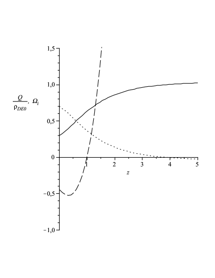
Figure 1: We show the evolution of the dimensionless energy densities $\Omega_{i}$ for dark matter (solid line), dark energy (dotted line) and the corresponding behavior of the coupling term $Q$ (dashed line) vs. redshift $z$ for the following values of the model parameters: $k=0$, $\alpha=-2$, $\beta=-1$, $\Omega_{{}_{DM0}}=0.3$, $\Omega_{{}_{DE0}}=0.7$, $\omega_{1}=-0.9$. In this case the interacting term $Q$ is negative for $z<1$, implying that for $z>1$ we have a transfer of energy from the dark matter to the dark energy, and for $z<1$ the energy is being transferred from the dark energy to the dark matter component.

It is interesting to note that the interacting term (15) now is given by

$$Q(a)=\frac{(\alpha+3(1+\omega_{1}))(\beta+3(1+\omega_{1}))\rho_{{}_{10}}}{3\omega_{1}(\beta-\alpha)}\left[-(\alpha+3)a^{\alpha-1}+(\beta+3)a^{\beta-1}\right].$$ (42)

Thus we have that it does not change sign only if $\alpha<-3$, $\beta>-3$ or $\alpha>-3$, $\beta<-3$. However in this case there are configurations leading to a negative energy density of the dark matter component.

It is interesting to remark that, as in Sec. IV-A, for any solution with $\omega_{2}=0$ we may find a set of cosmologies presenting a scaling behavior for energy densities at early and late epochs. Effectively, without any loss of generality let us suppose that $\beta<\alpha<0$, and then at late times the dark energy component will behave as $\rho_{{}_{DE}}\sim C_{1}a^{\alpha}$ while the dark matter component as $\rho_{{}_{DM}}\sim Ca^{-3}$ for $\alpha<-3$, or $\rho_{{}_{DM}}\sim\tilde{\tilde{C}}a^{\alpha}$ for $\alpha>-3$, where $\tilde{\tilde{C}}=\frac{\alpha+3(1+\omega_{1})}{3\omega_{1}(\beta-\alpha)}[(\beta+3(1+\omega_{1}))\rho_{{}_{DE0}}+(\rho_{{}_{DM0}}-C)(\beta+3)]$. Thus for $\alpha<-3$ we have for the ratio of energy densities $r=\frac{\rho_{{}_{DM}}}{\rho_{{}_{DE}}}\sim\frac{C}{C_{1}}a^{-(\alpha+3)}$. Clearly in this case $r$ diverges at late times, implying that the dark matter component dominates over the dark energy, so these models must be ruled out of consideration. On the other hand, for $\alpha>-3$ we have cosmological models with a scaling behavior since

$$r=\frac{\rho_{{}_{DM}}}{\rho_{{}_{DE}}}\sim-\frac{\alpha+3(1+\omega_{1})}{\alpha+3}=-1-\frac{3\omega_{1}}{\alpha+3},$$

thus alleviating the coincidence problem. In this case, in order to have $r>0$ we must require $\alpha+3(1+\omega_{1})<0$.

IV.3 The three-fluid interpretation

We next consider models in which there are two dark matter sectors: one describing the standard visible matter which is not interacting with the dark energy component, and another which is interacting with the dark energy. Both of these dark matter components are treated as pressureless fluids. The advantage of such a description is that we can describe the behavior of visible matter with an energy density which decreases with the scale factor as $\rho_{m}\sim a^{-3}$, while the energy density of the another dark matter component behaves as $\rho_{{}_{DM}}\sim a^{n}$, with $n<0$ and $n\neq-3$, in order that this second dark matter component also decreases with the scale factor.

Let us consider the general solution (9) and (10) with $\omega_{2}=0$. In this case we shall not consider the energy density $\rho_{2}$ in the normalized form (IV.2) and we shall write it in the following form:

$$\rho_{2}=\rho_{{}_{DM}}+\rho_{m},$$ (43)

where

$$\rho_{{}_{DM}}=-\frac{\alpha+3(1+\omega_{1})}{\alpha+3}\,C_{1}a^{\alpha}-\frac{\beta+3(1+\omega_{1})}{\beta+3}\,C_{2}a^{\beta},$$

$$\rho_{m}=\rho_{m0}a^{-3},\hskip 167.87108pt$$ (44)

and we have put $C=\rho_{m0}>0$. Note that, as in Sec. IV-B, the energy density of the dark energy is given by $\rho_{{}_{DE}}:=\rho_{1}$ of Eq. (9).

Thus, by putting expressions (IV.3) and (9) into the conservation equation (4), it may be rewritten as

$$\dot{\rho}_{{}_{DM}}+\dot{\rho}_{{}_{DE}}+3H(\rho_{{}_{DM}}+(1+\omega_{{}_{DE}})\rho_{{}_{DE}})=0,$$

$$\dot{\rho}_{m}+3H\rho_{m}=0,\hskip 2.84544pt$$ (45)

where we have put $\omega_{1}:=\omega_{{}_{DE}}$. Clearly the interpretation of these equations is different here: we have the conservation of the total visible matter $\rho_{m}$, while the dark matter is conserved together with the dark energy component. Therefore we can associate an interaction between $\rho_{{}_{DM}}$ and $\rho_{{}_{DE}}$. In this case the coupling between dark matter and dark energy is still given by Eq. (15).

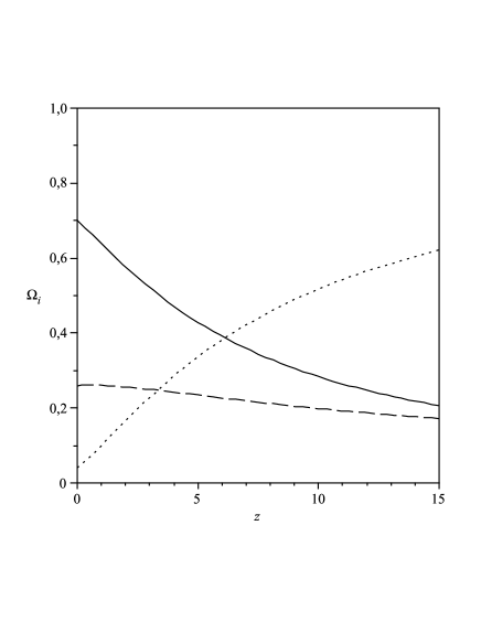
Figure 2: We show the behavior of the dimensionless energy densities $\Omega_{i}$ for standard visible matter (dotted line), dark matter (dashed line) and dark energy (solid line) for the following values of the model parameters: $k=0$, $\Omega_{m0}=0.04$, $\Omega_{{}_{DM0}}=0.26$, $\omega_{1}=-2/3$. This implies that $\beta<-1.542$ and $-1.542<\alpha<-1$. We have plotted curves for $\alpha=-3/2$ and $\beta=-5/2$. For late times the dark energy component dominates, while at early times dust is dominating.

Normalizing the solution in order to have today $\rho_{{}_{DM}}(a=1)=\rho_{{}_{DM0}}$ and $\rho_{{}_{DE}}(a=1)=\rho_{{}_{DE0}}$ the constants $C_{1}$ and $C_{2}$ may be written as

$$C_{1}=\frac{(\alpha+3)\left[(\beta+3)\rho_{{}_{DM0}}+(\beta+3(1+\omega_{1}))\rho_{{}_{DE0}}\right]}{3\omega_{1}(\alpha-\beta)},$$

$$C_{2}=-\frac{(\beta+3)\left[(\alpha+3)\rho_{{}_{DM0}}+(\alpha+3(1+\omega_{1}))\rho_{{}_{DE0}}\right]}{3\omega_{1}(\alpha-\beta)}.$$

It is clear that, if we want to have positive energy densities during all cosmic evolution, we must require that all terms of Eqs. (9) and (IV.3) must be positive. Thus, by requiring $C_{1}\geq 0$, $C_{2}\geq 0$, $\frac{\alpha+3(1+\omega_{1})}{\alpha+3}<0$, $\frac{\beta+3(1+\omega_{1})}{\beta+3}<0$ and without any lost of generality $\beta<\alpha$ we have that the following constraints must be satisfied for negative values of the state parameter $\omega_{1}$:

$$\frac{\beta+3(1+\omega_{1})}{\beta+3}<-\frac{\rho_{{}_{DM0}}}{\rho_{{}_{DE0}}},$$

$$-\frac{\rho_{{}_{DM0}}}{\rho_{{}_{DE0}}}<\frac{\alpha+3(1+\omega_{1})}{\alpha+3}<0.$$

This implies that the parameters $\alpha$ and $\beta$ are constrained to be

$$-\frac{3(1+r_{0}+\omega_{1})}{1+r_{0}}<\alpha<-3(1+\omega_{1}),$$

$$-3<\beta<-\frac{3(1+r_{0}+\omega_{1})}{1+r_{0}},$$ (47)

where $r_{0}=\frac{\rho_{{}_{DM0}}}{\rho_{{}_{DE0}}}$. It is clear that these constraints imply that energy is being transferred from dark energy to dark matter. Notice that for $C_{1}=0$ or $C_{2}=0$ we have that the energy densities of dark matter and dark energy are functions of the same power of the scale factor, i.e. $\rho_{{}_{DE}}/\rho_{{}_{DM}}=const$.

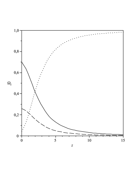
Figure 3: We show the behavior of the dimensionless energy densities $\Omega_{i}$ for standard visible matter (dotted line), dark matter (dashed line) and dark energy (solid line) for the following values of the model parameters: $k=0$, $\Omega_{m0}=0.04$, $\Omega_{{}_{DM0}}=0.26$, $\omega_{1}=-1.2$. This implies that $\beta<-0.375$ and $-0.375<\alpha<0$ and we have plotted curves for $\alpha=-0.3$ and $\beta=-1/2$. For late times the dark energy component dominates, while at early times dust is dominating. Note that in this case the dust-dark energy equality and dust-dark matter equality occur for $z\thickapprox 2$ and $z\thickapprox 1$ respectively.

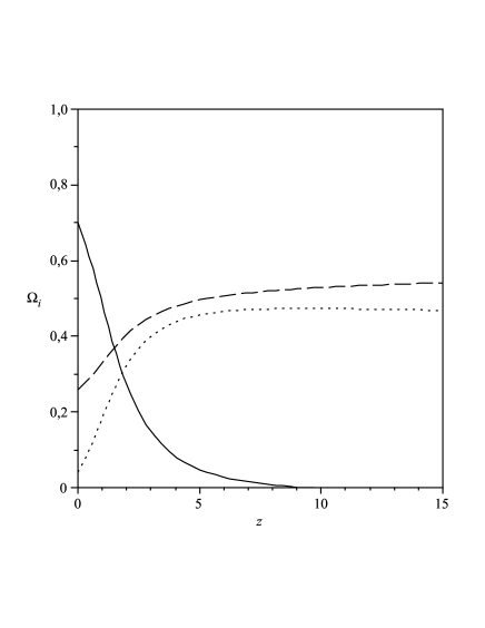
Figure 4: We show the behavior of the dimensionless energy densities $\Omega_{i}$ for standard visible matter (dotted line), dark matter (dashed line) and dark energy (solid line) for $k=0$, $\Omega_{m0}=0.04$, $\Omega_{{}_{DM0}}=0.26$, $\omega_{1}=-1.2$, $\alpha=-0.275$ and $\beta=-3.1$. In this case the dark energy density becomes negative for $z\gtrsim 9$ and the dust-dark energy equality occurs for $z\thickapprox 1.5$, while for $z\thickapprox 2$ we have the dark energy-dark matter equality. Notice that for $z\gtrsim 5$ the energy is transferred from the dark matter to dark energy, and for $z\lesssim 5$ is from dark energy to dark matter.

In Figs. 2 and 3 are plotted the evolution of three dimensionless energy densities $\Omega_{m}$, $\Omega_{{}_{DM}}$ and $\Omega_{{}_{DE}}$ ($\Omega_{m}+\Omega_{{}_{DM}}+\Omega_{{}_{DE}}=1$) in the case of flat FRW cosmologies ($k=0$) and always positive dark energy and dark matter energy densities. In order to have an estimation for the behavior of dimensionless energy densities, the cosmological model parameters are fixed to take the values $\Omega_{{}_{m0}}=0.04$ and $\Omega_{{}_{DM0}}=0.26$, which are in good agreement with a wide range of observations OBSDM ; OBSDM1 ; OBSDM2 . In both cases the energy is transferred from the dark energy to the dark matter.

If we do not exclude the possibility of negative energies we can also consider cases where the dark energy becomes negative at some stage during the cosmic evolution. For example in Fig. 4 we show the case where negative values for the dark energy density are allowed at early times. However it must be noticed that the total energy density $\rho_{{}_{tot}}=\rho_{m0}+\rho_{{}_{DM0}}+\rho_{{}_{DE0}}$ is positive during all cosmic evolution. An interesting feature of such a scenario with negative energy is that we have a period where the energy is transferred from dark energy to dark matter and another where this occurs from the dark matter component to dark energy.

V conclusions

In this paper we have studied Friedmann-Robertson-Walker cosmological models with matter content composed of two barotropic perfect fluids where one of the energy densities is given by a sum of two powers of the scale factor of the form of Eq. (9). By associating with these cosmologies an interacting term $Q$, it can be shown that interacting scenarios with couplings given by $Q=\tilde{\alpha}H\rho_{1}$, $Q=\tilde{\alpha}H\rho_{2}$, $Q=\tilde{\alpha}H(\rho_{1}+\rho_{2})$ and $Q=\tilde{\alpha}H\rho_{1}+\tilde{\beta}H\rho_{2}$ (with constants $\tilde{\alpha}$ and $\tilde{\beta}$) correspond to particular cases of our cosmological model. The studied cosmological models contain a class of solutions having a scaling behavior at early and at late times, and then the coincidence problem is substantially alleviated.

It is interesting to note that in the framework of the considered scenarios it is possible to introduce a three fluid interpretation, where one fluid describes the standard visible matter and is conserved separately from the dark matter and dark energy components, which are conserved together. If we want to introduce the interacting picture, thus the visible matter is not interacting neither with the dark matter nor dark energy components, while these latter two components are interacting with each other. In this case, if energy densities of dark matter and dark energy are positive during all cosmic evolution, then the energy always is transferred from the dark energy component to dark matter in agreement with the conclusions of Ref. Pavon2007 .

It is remarkable that the inequalities (IV.3) impose a lower limit on the values of the state parameter $\omega_{1}$. Effectively, if we require that the energy density of the dark matter be decreasing with the expansion, i.e. $\alpha<0$ and $\beta<0$, then the state parameter is constrained to be in the range $\omega_{1}>-(1+r_{0})$. Thus, in agreement with the observations, we have for the ratio $r_{0}=\frac{\rho_{{}_{DM0}}}{\rho_{{}_{DE0}}}=\frac{\Omega_{{}_{DM0}}}{\Omega_{{}_{DE0}}}=0.26/0.7$ and then $\omega_{1}>-1.371$. Note that this constraint on the state parameter $\omega_{1}$ is allowed in this model by the requirement of positivity of energy densities of dark matter and dark energy during all cosmic evolution. However, one can impose more stringent constraints on the model parameters by using for example the latest supernova data. In order to do this we shall use the recent compilation of SNe Ia data called the Union data set Kowalski , which contains a set of 57 nearby ($0.015<z<0.15$) Type Ia supernovae, and 250 high-redshift supernovae. The $\chi^{2}$ statistic is quite helpful in constraining the parameter values of a given model LVerde . In our case this method will allow us to fit the set of the model parameters $\alpha$, $\beta$ and $\omega_{1}$ to the set of cosmological parameters of the Union compilation data, by finding the best fit values of the model parameters by minimizing this $\chi^{2}$. In this case the minimum of $\chi^{2}$ should be roughly equal to the number of data, or the so-called “reduced chisquare” $\chi^{2}_{\nu}=\chi^{2}_{min}/307$ should be roughly equal to 1.

In Fig. 5 we show the probability contours from the above $307$ data points only at $68.3\%$, $95.4\%$ and $99.7\%$ confidence levels (from inside to outside) in the $\alpha-\omega_{1}$ plane for the value $\beta=-5/2$ of Fig. 2. In this case the best-fitting parameters are $\alpha=-0.1$ and $\omega_{1}=-0.97$ with $\chi^{2}_{\nu}=1.021$, implying the constraints $-3.6\lesssim\alpha\lesssim 3.4$ and $-1.49\lesssim\omega_{1}\lesssim-0.45$ ($99.7\%$ C.L.). Note that in this case, by taking into account the above constraint on the state parameter $\omega_{1}$, we can rewrite the latter constraint as $-1.371<\omega_{1}\lesssim-0.45$.

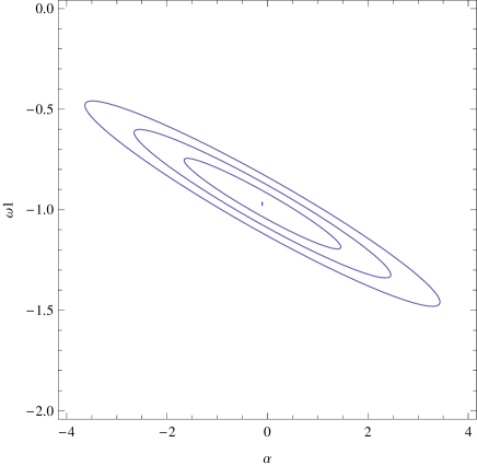
Figure 5: We show the probability contours at $68.3\%$, $95.4\%$ and $99.7\%$ confidence levels in the $\alpha-\omega_{1}$ plane for the value $\beta=-5/2$ of Fig. 2. In this case the best-fitting parameters are $\alpha=-0.1$ and $\omega_{1}=-0.97$ with $\chi^{2}_{\nu}=1.021$.

In Fig. 6 we show the probability contours at $68.3\%$, $95.4\%$ and $99.7\%$ confidence levels (from inside to outside) in the $\alpha-\beta$ plane for the value $\omega_{1}=-1.2$ of Fig. 3 and Fig. 4. In this case the best-fitting parameters are $\alpha=0.59$ and $\beta=-2.99$ with $\chi^{2}_{\nu}=1.024$, implying the constraints $-0.34\lesssim\alpha\lesssim 1.52$ and $-4.65\lesssim\beta\lesssim-1.33$ ($99.7\%$ C.L.). Thus, in this case, in order to have a decreasing with expansion dark matter energy density, we must require that $-3<\beta\lesssim-1.33$ and $-0.34\lesssim\alpha<0$.

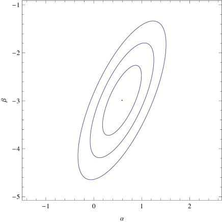
Figure 6: We show the probability contours at $68.3\%$, $95.4\%$ and $99.7\%$ confidence levels (from inside to outside) in the $\alpha-\beta$ plane for the value $\omega_{1}=-1.2$ of Fig. 2. In this case the best-fitting parameters are $\alpha=0.59$ and $\beta=-2.99$ with $\chi^{2}_{\nu}=1.024$.

Lastly, in Fig. 7 we show the evolution of the Hubble parameter $H(z)/H_{0}$ vs. the redshift $z$ for $\omega_{1}=-1$, while in Figs. 8, 9 and 10 we show the evolution of the deceleration parameter $q$ vs. redshift $z$ for some values of the state parameter $\omega_{1}$ ($-1.371<\omega_{1}<-1/3$). Note that in Fig. 10, for comparison, the prediction of the $\Lambda$CDM model is also shown.

VI Acknowledgements

This work was supported by CONICYT through Grant FONDECYT N⁰ 1080530 (MC), PhD Grant N⁰ 21070949 (FA) and by Dirección de Investigación de la Universidad del Bío–Bío (MC).

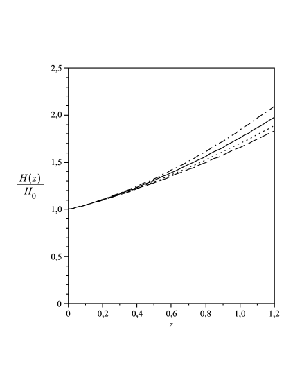
Figure 7: We show the evolution of the Hubble parameter with the redshift $z$ for $k=0$, $\Omega_{m0}=0.04$, $\Omega_{{}_{DM0}}=0.26$, $\beta=-0.05$, $\omega_{1}=-1$ and $\alpha=-2.6$ (dashed line), $\alpha=-2.8$ (dotted line) and $\alpha=-3.4$ (dashdotted line). For comparison, the prediction of the $\Lambda$CDM model (solid line) is also shown.

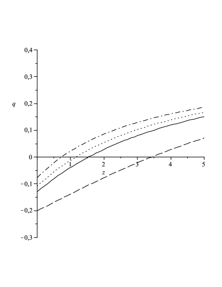
Figure 8: We show the evolution of the deceleration parameter $q$ with the redshift $z$ for $k=0$, $\Omega_{m0}=0.04$, $\Omega_{{}_{DM0}}=0.26$, $\alpha=-3/2$ and $\beta=-5/2$, and $\omega_{1}=-0.55$ (dashdotted line), $\omega_{1}=-0.58$ (dotted line), $\omega_{1}=-0.6$ (solid line) and $\omega_{1}=-2/3$ (dashed line). In this case the value of the redshift $z$, for transition from decelerated expansion to accelerated expansion, becomes smaller with the increase of the state parameter $\omega_{1}$.

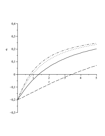
Figure 9: We show the evolution of the deceleration parameter $q$ with the redshift $z$ for $k=0$, $\Omega_{m0}=0.04$, $\Omega_{{}_{DM0}}=0.26$, $\beta=-5/2$, $\omega_{1}=-2/3$, and $\alpha=-3/2$ (dashed line), $\alpha=-1.2$ (solid line), $\alpha=-1$ (dotted line) and $\alpha=-0.9$ (dashdotted line). In this case the value of the redshift $z$, for transition from decelerated expansion to accelerated expansion, becomes smaller with the increase of the parameter $\alpha$.

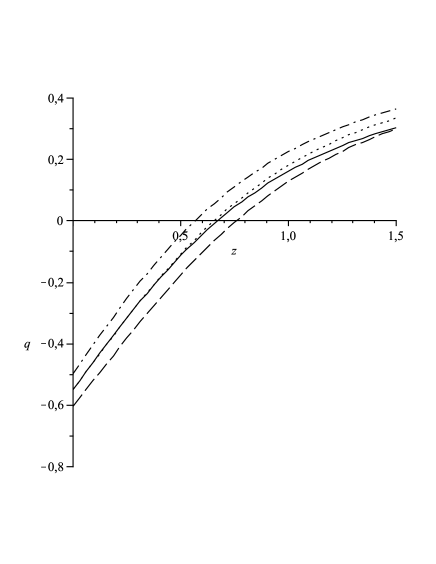
Figure 10: We show the evolution of the deceleration parameter $q$ with the redshift $z$ for $k=0$, $\Omega_{m0}=0.04$, $\Omega_{{}_{DM0}}=0.26$, $\alpha=-3.1$, $\beta=-0.05$, and $\omega_{1}=-1.05$ (dashed line), $\omega_{1}=-1$ (dotted line) and $\omega_{1}=-0.95$ (dashdotted line). For comparison, the prediction of the $\Lambda$CDM model (solid line) is also shown.

References

- (1) A. Avelino and U. Nucamendi, JCAP 0904, 006 (2009); Y. F. Cai and J. Wang, Class. Quant. Grav. 25, 165014 (2008); M. Jamil and M. A. Rashid, Eur. Phys. J. C 56, 429 (2008); J. Ren and X. H. Meng, Int. J. Mod. Phys. D 17, 2325 (2008); G. Panotopoulos, Nucl. Phys. B 796, 66 (2008); E. J. Copeland, M. Sami and S. Tsujikawa, Int. J. Mod. Phys. D 15, 1753 (2006); I. H. Brevik and O. Gorbunova, Gen. Rel. Grav. 37, 2039 (2005); I. H. Brevik and O. Gorbunova, Gen. Rel. Grav. 37, 2039 (2005); J. A. S. Lima and J. S. Alcaniz, Astrophys. J. 566, 15 (2002); K. Bamba, C. Q. Geng, S. Nojiri and S. D. Odintsov, arXiv:0810.4296 [hep-th].
- (2) R. R. Caldwell, Phys. Lett. B 545, 23 (2002); S. Nojiri and S. D. Odintsov, Phys. Lett. B 562, 147 (2003); P. Singh, M. Sami and N. Dadhich, Phys. Rev. D 68, 023522 (2003); A. Vikman, Phys. Rev. D 71, 023515 (2005); M. P. Dabrowski, T. Stachowiak and M. Szydlowski, Phys. Rev. D 68, 103519 (2003); L. P. Chimento and R. Lazkoz, Phys. Rev. Lett. 91, 211301 (2003); P. F. Gonzalez-Diaz, Phys. Rev. D 68, 021303 (2003); R. Curbelo, T. Gonzalez and I. Quiros, Class. Quant. Grav. 23, 1585 (2006).
- (3) R. G. Cai and A. Wang, JCAP 0503, 002 (2005); W. Zimdahl and D. Pavon, Gen. Rel. Grav. 36, 1483 (2004); S. Dodelson, M. Kaplinghat and E. Stewart, Phys. Rev. Lett. 85, 5276 (2000).
- (4) C. G. Boehmer, G. Caldera-Cabral, R. Lazkoz and R. Maartens, hys. Rev. D 78, 023505 (2008); B. Wang, J. Zang, C. Y. Lin, E. Abdalla and S. Micheletti, Nucl. Phys. B 778, 69 (2007); V. Sahni, Lect. Notes Phys. 653, 141 (2004); M. S. Turner, Phys. Scripta T85, 210 (2000).
- (5) G. Olivares, F. Atrio-Barandela and D. Pavon, Phys. Rev. D 71, 063523 (2005).
- (6) G. R. Farrar and P. J. E. Peebles, Astrophys. J. 604, 1 (2004). R. Rosenfeld, Phys. Rev. D 75, 083506 (2007); Z. K. Guo, N. Ohta and S. Tsujikawa, Phys. Rev. D 76, 023508 (2007).
- (7) Z. K. Guo, N. Ohta and S. Tsujikawa, Phys. Rev. D 76, 023508 (2007); L. Amendola, G. Camargo Campos and R. Rosenfeld, Phys. Rev. D 75, 083506 (2007).
- (8) M. Cataldo, P. Mella, P. Minning and J. Saavedra, Phys. Lett. B 662, 314 (2008).
- (9) J. H. He and B. Wang, JCAP 0806, 010 (2008).
- (10) J. D. Barrow and T. Clifton, Phys. Rev. D 73, 103520 (2006); T. Clifton and J. D. Barrow, Phys. Rev. D 75, 043515 (2007).
- (11) L. P. Chimento, A. S. Jakubi, D. Pavón and W. Zimdahl, Phys. Rev. D 67, 083513 (2003); W. Zimdahl, D. Pavón, and L.P. Chimento, Phys. Lett. B 521, 133 (2001).
- (12) L. Amendola, G. Camargo Campos and R. Rosenfeld, Phys. Rev. D 75, 083506 (2007).
- (13) W. J. Percival et al. [The 2dFGRS Collaboration], Mon. Not. Roy. Astron. Soc. 327, 1297 (2001); J. A. Peacock arXiv:astro-ph/0105450.
- (14) J. J. Mohr, E. D. Reese, E. Ellingson, A. D. Lewis and A. E. Evrard, arXiv:astro-ph/0004242; D. O. Caldwell, arXiv:hep-ph/9910349.
- (15) Perlmutter, S., et al, Astrophys. J. 517, 565 (1998); Riess, A.G., Astron. J, 116, 1009 (1998).
- (16) D. Pavon and B. Wang, Gen. Rel. Grav. 41, 1 (2009).
- (17) M. Kowalski et al. [Supernova Cosmology Project Collaboration], Astrophys. J. 686, 749 (2008).
- (18) L. Verde, arXiv:0911.3105 [astro-ph.CO]; arXiv:0712.3028 [astro-ph].