Ground state of two electrons on a sphere
Abstract
We have performed a comprehensive study of the singlet ground state of two electrons on the surface of a sphere of radius . We have used electronic structure models ranging from restricted and unrestricted Hartree-Fock theory to explicitly correlated treatments, the last of which lead to near-exact wavefunctions and energies for any value of . Møller-Plesset energy corrections (up to fifth-order) are also considered, as well as the asymptotic solution in the large- regime.
pacs:
31.15.ac, 31.15.ve, 31.15.xp, 31.15.xr, 31.15.xtI Introduction
Exactly (or very accurately) solvable models have ongoing value and are valuable both for illuminating more complicated systems and for testing theoretical approaches, such as density functional methods Hohenberg and Kohn (1964); Kohn and Sham (1965); Parr and Yang (1989). One such model is the Hooke’s law atom (or Harmonium) which is composed of two electrons bound to a nucleus by a harmonic potential but repelling Coulombically. This system was first considered more than 40 years ago by Kestner and Sinanoglu Kestner and Sinanoglu (1962), but solved analytically in 1989 by Kais et al. Kais et al. (1989) for a particular value of the harmonic force constant and, later, for a countably infinite set force constants Taut (1993).
A related system, studied by Alavi and co-workers Alavi (2000); Thompson and Alavi (2002, 2005), consists of two electrons, interacting through a Coulomb potential, but confined within a ball of radius . This possesses a number of interesting features, including the formation of a “Wigner molecule” for large Thompson and Alavi (2004). The spontaneous formation of such molecules can also occur in quantum dots and is analogous to the Wigner crystallization Wigner (1934) of the uniform electron gas.
If the two electrons are constrained to remain on the surface of the sphere, one obtains a model that Berry and co-workers have used Ezra and Berry (1982, 1983); Ojha and Berry (1987); Hinde and Berry (1990) to understand both weakly and strongly correlated systems, such as the ground and excited states of the helium atom, and also to suggest the “alternating” version of Hund’s rule Warner and Berry (1985). Seidl studied this system in the context of density functional theory Seidl (2007a) in order to test the ISI (interaction-strength interpolation) model Seidl et al. (2000). For this purpose, he derived accurate solutions in both the weak interaction limit (the small regime) and the strong interaction limit (the large regime). He also obtained accurate results by numerical integration of the Schrödinger equation.
In this paper, we are interested in the ground state of two electrons on the surface of a sphere of radius . This allows us to restrict our study to the symmetric spatial part of the wavefunction and ignore the spin coordinates. We have extended Seidl’s analysis and performed an exhaustive study using a range of models. We restrict our analysis to the repulsive potential case; the strong-attraction limit (attractive potential) is carefully examined in Ref. Seidl (2007a).
Restricted and unrestricted Hartree-Fock (HF) solutions are discussed in Section III and the strengths and weaknesses of Møller-Plesset (MP) perturbation theory Møller and Plesset (1934) in Section IV. We consider asymptotic solutions for large in Section V and, in Section VI, we explore several variational schemes including explicitly correlated techniques Hylleraas (1964); Kutzelnigg (1985); Klopper and Kutzelnigg (1987, 1990); Kutzelnigg and Klopper (1991)) that enforce the cusp condition Kato (1957); Pack and Byers Brown (1966). Atomic units are used throughout.
II Hamiltonian
The absolute position of the -th electron is defined by its spherical polar angles . The relative position of the electrons is conveniently measured by the interelectronic angle which they subtend at the origin. These coordinates are related by
| (1) |
and we have .
The Hamiltonian is
| (2) |
where
| (3) |
is the kinetic operator for both electrons and is the Coulomb operator. In terms of , the Hamiltonian is
| (4) |
in which form it becomes clear that the kinetic and potential parts of scale with and , respectively.
III Hartree-Fock approximations
III.1 Restricted Hartree-Fock
In the HF approximation, each electron feels the mean field generated by the other electron Szabo and Ostlund (1989). The restricted Hartree-Fock (RHF) solution
| (5) |
places both electrons in an orbital that is an eigenfunction of the Fock operator
| (6) |
with .
By definition, the one-electron basis function
| (7) |
where is the spherical harmonic of degree and order is an eigenfunction of with eigenvalue . Using the partial-wave expansion Arfken (1966)
| (8) |
and the addition theorem Abramowitz and Stegun (1972)
| (9) |
it is straightforward to show that
| (10) |
The orbital is thus an eigenfunction of with the eigenvalue . Moreover, it follows from the orthogonality of the spherical harmonics that
| (11) |
which ensures the stationarity of the RHF energy with respect to the orbitals .
The ground-state RHF energy is thus
| (12) |
and the normalized RHF wavefunction is
| (13) |
which yields a uniform electron density over the surface of the sphere.
III.2 Unrestricted Hartree-Fock
When exceeds a critical value, a second, unrestricted HF (UHF) solution develops Cizek and Paldus (1967); Paldus and Cizek (1970); Seeger and Pople (1977) in which the two electrons tend to localize on opposite sides of the sphere. This is analogous to the UHF description of a dissociating H2 molecule Szabo and Ostlund (1989).
To obtain this symmetry-broken solution
| (14) |
we expand the orbital as
| (15) |
where the are zonal spherical harmonics. The Fock matrix elements in this basis are
| (16) |
where the two-electron integrals are
| (17) |
Using the partial-wave expansion (8) and the relation
| (18) |
between the integrals of three spherical harmonics and the Wigner 3j-symbols Edmonds (1957), we find
| (19) |
where selection rules Edmonds (1957) restrict the terms in the sum.
The UHF energy is then given by
| (20) |
The first term is the kinetic energy and is positive. However, for sufficiently large , this is outweighed by negative contributions in the second term and it is these that drive the symmetry-breaking process.
For computational reasons, we truncate the sum in (15) at but, for all of the radii considered in this study, we found that suffices to obtain with an accuracy of .
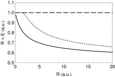
As Table 1 and Figure 1 show, the UHF solution becomes lower than the RHF one for and the UHF, not RHF, energy behaves correctly for large . Specifically, it can be shown that
| (21) | |||
| (22) |
The UHF result reflects the Coulomb interaction between two electrons localized on opposite sides of the sphere Seidl (2007a), a phenomenon known as Wigner crystallization Thompson and Alavi (2004); Wigner (1934). The difference between the UHF and exact energies (i.e. the correlation energy) appears to decay as .
| 0.0001 | 10000 | 10000 | 9999.772 600 495 |
| 0.001 | 1000 | 1000 | 999.772 706 409 |
| 0.01 | 100 | 100 | 99.773 761 078 |
| 0.1 | 10 | 10 | 9.783 873 673 |
| 0.2 | 5 | 5 | 4.794 237 154 |
| 0.5 | 2 | 2 | 1.820 600 768 |
| 1 | 1 | 1 | 0.852 781 065 |
| 2 | 0.500 000 | 0.489 551 | 0.391 958 796 |
| 3 | 0.333 333 | 0.304 783 | 0.247 897 526 |
| 4 | 0.250 000 | 0.215 864 | 0.179 210 308 |
| 5 | 0.200 000 | 0.165 161 | 0.139 470 826 |
| 10 | 0.100 000 | 0.072 829 | 0.064 525 123 |
| 20 | 0.050 000 | 0.032 983 | 0.030 271 992 |
| 50 | 0.020 000 | 0.012 006 | 0.011 363 694 |
| 100 | 0.010 000 | 0.005 708 105 | 0.005 487 412 |
| 1000 | 0.001 000 | 0.000 522 363 | 0.000 515 686 |
IV Expansion for small R
In Møller-Plesset perturbation theory, the Hamiltonian of the system is partitioned as
| (23) |
where the zeroth-order Hamiltonian and is a perturbation operator and, in our case, we have
| (24) | ||||
| (25) |
The ground-state wavefunction and energy are expanded
| (26) | |||
| (27) |
We will refer to as the th-order energy and define the MP correlation energy as
| (28) |
Dimensional analysis reveals that
| (29) | |||
| (30) |
where the are functions of and the are numbers. From (12) and (13), we see , and .
The excited eigenfunctions of are given by
| (31) |
and we can expand the exact wavefunction in this basis. However, for the ground state, angular momentum theory Edmonds (1957); Slater (1960) limits the combinations of , , and that contribute and it is more efficient to expand in the basis of two-electron functions
| (32) |
which are eigenfunctions of with eigenvalues
| (33) |
IV.1 First-order wavefunction
In the intermediate normalization, the first-order wavefunction is
| (34) |
Using the Legendre generating function
| (35) |
the sum in (IV.1) can be found in closed-form, yielding
| (36) |
or, equivalently,
| (37) |
and these yield the normalized first-order wavefunction
| (38) |
The true ground-state wavefunction must be nodeless. However, it is easy to show that the MP1 wavefunction possesses a node if , leading us to anticipate that will be a poor wavefunction for large spheres.
IV.2 Second- and third-order energies
According to the Wigner rule Helgaker et al. (2000), the 1st-order wavefunction generates the 2nd- and 3rd-order energies. The 2nd-order energy, which has previously been found by Seidl Seidl (2007a), is given by
| (39) |
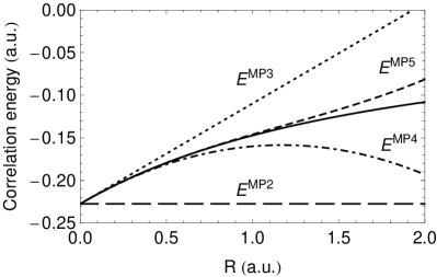
where . As Table 2 shows, the MP2 correlation energy is an excellent approximation for small but, because it is independent of , it is poor for large .
It is surprising to find that is so much larger than the limiting correlation energies Gill and O’Neill (2005) of the helium-like ions () or Hooke’s Law atoms ().
The 3rd-order energy is given by
| (40) |
and this yields
| (41) |
which agrees with Seidl’s rough estimate Seidl (2007a). Table 2 shows that MP3 gives an improvement over MP2 but that it, too, eventually breaks down as increases.
| R | MP2 | MP3 | MP4 | MP5 | Hylleraas | Seidl | Exact111From the polynomial wavefunction in Section VI.4 |
| 0.0001 | 0.227 411 | 0.227 399 504 071 | 0.227 399 504 574 | 0.227 399 504 574 | 0.222 212 | — | 0.227 399 504 574 |
| 0.001 | 0.227 411 | 0.227 293 541 | 0.227 293 591 147 | 0.227 293 591 133 | 0.222 123 | — | 0.227 293 591 133 |
| 0.01 | 0.227 411 | 0.226 234 | 0.226 238 936 | 0.226 238 922 473 | 0.221 237 | — | 0.226 238 922 463 |
| 0.1 | 0.227 411 | 0.215 638 | 0.216 140 | 0.216 126 387 | 0.212 574 | 0.2175222Native result of Ref. Seidl (2007a). | 0.216 126 326 630 |
| 0.2 | 0.227 411 | 0.203 864 | 0.205 875 | 0.205 763 261 | 0.203 406 | 0.2064222Native result of Ref. Seidl (2007a). | 0.205 762 846 030 |
| 0.5 | 0.227 411 | 0.168 543 | 0.181 112 | 0.179 367 | 0.178 908 | 0.1796222Native result of Ref. Seidl (2007a). | 0.179 399 232 168 |
| 1 | 0.227 411 | 0.109 674 | 0.159 950 | 0.145 992 | 0.147 181 | 0.1473222Native result of Ref. Seidl (2007a). | 0.147 218 934 944 |
| LR0 | LR1 | LR2 | |||||
| 2 | 0.239 551 | 0.062 774 | 0.094 024 | 0.095 405 | 0.096 444 | 0.0977333Correlation energy form Ref. Seidl (2007a) relative to the UHF energy. | 0.097 591 955 594 |
| 3 | 0.138 116 | 0.041 890 | 0.055 780 | 0.056 281 | 0.054 783 | — | 0.056 885 070 442 |
| 4 | 0.090 864 | 0.028 352 | 0.036 176 | 0.036 420 | 0.033 984 | — | 0.036 653 426 934 |
| 5 | 0.065 161 | 0.020 440 | 0.025 440 | 0.025 580 | 0.022 707 | 0.0257333Correlation energy form Ref. Seidl (2007a) relative to the UHF energy. | 0.025 690 364 031 |
| 10 | 0.022 829 | 0.007 018 | 0.008 268 | 0.008 292 | 0.005 129 | 0.0083333Correlation energy form Ref. Seidl (2007a) relative to the UHF energy. | 0.008 303 955 973 |
| 20 | 0.007 983 | 0.002 393 | 0.002 706 | 0.002 710 | 0.000 154 | — | 0.002 711 198 384 |
| 50 | 0.002 006 | 0.000 592 | 0.000 642 054 | 0.000 642 496 | -0.000 860 | — | 0.000 642 573 605 |
| 100 | 0.000 708 | 0.000 187 | 0.000 220 605 | 0.000 220 683 | -0.000 679 | — | 0.000 220 692 615 |
| 1000 | 0.000 022 | 0.000 006 552 | 0.000 006 677 055 | 0.000 006 677 302 | -0.000 112 | — | 0.000 006 677 311 |
IV.3 Second-order wavefunction
To find the 4th- and 5th-order energies, we need the 2nd-order wavefunction. This is given by
| (42) |
which yields
| (43) |
Using the identity
| (44) |
for , we eventually obtain
| (45) |
where is the dilogarithm function Lewin (1958).
IV.4 Fourth- and fifth-order energies
The Wigner rule and the closed-form expression of yield the 4th- and 5th-order coefficients
| (46) | ||||
| (47) |
where is the Riemann zeta function.
The MP correlation energies for various values of are reported in Table 2 and illustrated in Figure 2. The results show that MP4 and MP5 are very accurate for small and, indeed, the latter is reasonable up to .
The MP expansion converges for radii within the radius of convergence
| (48) |
From our results, it seems that , but it is not possible to be more precise than this Seidl et al. (2000); Seidl (2007a).
V Expansion for large R
V.1 Harmonic approximation
For large (LR), the potential dominates the kinetic energy and the electrons tend to localize on opposite sides of the sphere. The classical mechanical energy would be
| (49) |
but, quantum mechanically, the kinetic energies of the electrons cannot vanish and each electron therefore maintains a zero-point oscillation around its equilibrium position with an angular frequency . Such phenomena are ubiquitous in strongly correlated systems, as demonstrated by Seidl and his co-workers Seidl et al. (1999); Seidl (1999); Seidl et al. (2000); Seidl (2007b, a).
In this limit, the supplementary angle is the natural coordinate and the Hamiltonian becomes
| (50) |
For small oscillations (), the Taylor series
| (51) | |||
| (52) |
yield the harmonic-oscillator Hamiltonian
| (53) |
whose ground-state wavefunction and energy are
| (54) | |||
| (55) |
The second term is the zero-point energy associated with harmonic oscillations of angular frequency and it appears that this is the leading error in the UHF description at large .
V.2 First and second anharmonic corrections
By analogy with the small- expansion (30), we would like to construct a large- asymptotic expansion
| (56) |
where we know . The th excited state of the Hamiltonian (53) has the wavefunction and energy
| (57) | |||
| (58) |
where is the Laguerre polynomial of degree Abramowitz and Stegun (1972). The anharmonic corrections, and , can be found Bender and Wu (1969) using the perturbation operators
| (59) | ||||
| (60) |
The first-order correction is
| (61) |
and this yields and therefore
| (62) |
The second-order correction is
| (63) |
but because of the orthogonality and recurrence relations of Laguerre polynomials Abramowitz and Stegun (1972), only the first two terms in the sum in (63) are non-zero and one finds and therefore
| (64) |
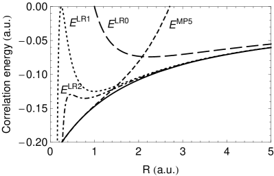
From the results in Table 2 and Figure 3, it seems that the asymptotic expansion converges toward the exact energy and is reasonably accurate for .
Through judicious use of the 5th-order truncation of (30) and the 2nd-order truncation of (V.2), one can predict satisfactory energies over a wide range of values. However, there remains a region () where both the small- and large- solutions are inadequate.
VI Variational wavefunctions
VI.1 Configuration interaction
We begin with a configuration interaction (CI) treatment wherein the wavefunction is expanded as
| (65) |
in the Legendre polynomial basis set (32). The resulting energy is the lowest eigenvalue of the CI matrix
| (66) |
where is defined by (III.2).
The CI energy as the maximum angular momentum increases is reported in Table 3. It converges very slowly and even yields an accuracy of only . The reason for this slow convergence – the failure of (65) to satisfy the Kato cusp condition – is well known.
| CI | R12-CI | Polynomial | |
|---|---|---|---|
| 0 | |||
| 1 | |||
| 2 | |||
| 3 | |||
| 4 | |||
| 5 | |||
| 10 | |||
| 15 | |||
| 20 | |||
| 25 | |||
| 30 | |||
| 35 | |||
| 40 |
VI.2 Hylleraas
The simplest possible wavefunction with a cusp is
| (67) |
which has an explicit linear dependence on the interelectronic distance . Kato proved Kato (1957) that in normal singlet states but, because our electrons are confined to a sphere, this does not apply (see below).
Using the partial-wave expansion
| (68) |
one finds that the energy is
| (69) |
and minimizing this with respect to yields
| (70) | |||
| (71) |
Correlation energies obtained from (71) for several values of are reported in Table 2. Despite the simplicity of the wavefunction, its energies are surprisingly good with a maximum deviation of for large and for small . As tends to zero, the correlation energy approaches , which is close to the exact value . However, as becomes large, one can show that which lies between the RHF and UHF energies. The Hylleraas wavefunction is thus a useful alternative to the small- and large- solutions in the problematic intermediate region () with errors of 0.000, 0.0011 and 0.0021 for 1, 2 and 3, respectively.
VI.3 R12-CI
Using the Hylleraas wavefunction (67) as the reference for a CI expansion yields the R12-CI wavefunction
| (72) |
where
| (73) |
is a projection operator that ensures orthogonality between the reference wavefunction and the excited determinants and is the identity operator. The coupling coefficients between two basis functions are the same as those for the conventional CI calculation (66) but with a correction for the matrix element
| (74) |
involving the ground state and the excited determinants. It is no longer possible to optimize in closed form so we used the value given by (70).
As Table 3 shows, the R12-CI energies converge much more rapidly with than the CI energies and, for example, is more accurate than . This illustrates the importance of including a term that is linear in . However, although this term enhances the initial convergence rate, the asymptotic behavior of the CI and R12-CI schemes are identical. Therefore, we now investigate the effect of including higher-order terms.
VI.4 Polynomial
In terms of the distance , the Hamiltonian is
| (75) |
and a Kato-like analysis Kato (1957) reveals the cusp condition
| (76) |
which deviates from the normal value of 1/2 Seidl (2007a).
The natural generalization of the Hylleraas wavefunction (67) is a polynomial and it is convenient to select the orthonormal basis of Jacobi polynomials Abramowitz and Stegun (1972)
| (77) |
and write the wavefunction as
| (78) |
The energy is the lowest eigenvalue of the matrix
| (79) |
where and .
Table 3 reveals the remarkable convergence of . Using and , for example, we find
| (80) |
The convergence is slower for larger values of , but still impressive. For example, using and , the energy is still correct to 49 digits. The ease with which we can obtain these Schrödinger eigenvalues can be traced to the fact that the polynomial basis efficiently models all of the singularities (the 1st-order cusp, the third-order cusp, etc.) in the exact wavefunction.
VII Conclusion
In this article, we have reported results for the ground state of a simple two-electron system that is described by a single parameter . Although we cannot solve its Schrödinger equation in closed form, we have found accurate wavefunctions and energies for small (the weakly correlated limit) and large (the strongly correlated limit). For , Møller-Plesset perturbation theory yields results close to the exact solution; for , accurate results can be found by considering the zero-point oscillations of the appropriate Wigner molecule.
We have also explored variational schemes that yield satisfactory results for all . In particular, we have discovered a polynomial wavefunction that easily yields results of any required accuracy.
We believe that our results will be useful in the future development of accurate correlation functionals within density-functional theory Sun (2009); Gori-Giorgi et al. (2009) and intracule functional theory Gill et al. (2005); Dumont et al. (2007); Crittenden and Gill (2007); Crittenden et al. (2007); Bernard et al. (2008); Pearson et al. (2009).
Acknowledgements.
PMWG thanks the APAC Merit Allocation Scheme for a grant of supercomputer time and Australian Research Council (Grant DP0664466) for funding. We also thank Yves Bernard for helpful comments on the manuscript, and fruitful discussions.References
- Hohenberg and Kohn (1964) P. Hohenberg and W. Kohn, Phys. Rev. B 136, 864 (1964).
- Kohn and Sham (1965) W. Kohn and L. Sham, Phys. Rev. A 140, 1133 (1965).
- Parr and Yang (1989) R. G. Parr and W. Yang, Density Functional Theory for Atoms and Molecules (Oxford University Press, 1989).
- Kestner and Sinanoglu (1962) N. R. Kestner and O. Sinanoglu, Phys. Rev. 128, 2687 (1962).
- Kais et al. (1989) S. Kais, D. R. Herschbach, and R. D. Levine, J. Chem. Phys 91, 7791 (1989).
- Taut (1993) M. Taut, Phys. Rev. A 48, 3561 (1993).
- Alavi (2000) A. Alavi, J. Chem. Phys. 113, 7735 (2000).
- Thompson and Alavi (2002) D. C. Thompson and A. Alavi, Phys. Rev. B 66, 235118 (2002).
- Thompson and Alavi (2005) D. C. Thompson and A. Alavi, J. Chem. Phys. 122, 124107 (2005).
- Thompson and Alavi (2004) D. C. Thompson and A. Alavi, Phys. Rev. B 69, 201302 (2004).
- Wigner (1934) E. Wigner, Phys. Rev. 46, 1002 (1934).
- Ezra and Berry (1982) G. S. Ezra and R. S. Berry, Phys. Rev. A 25, 1513 (1982).
- Ezra and Berry (1983) G. S. Ezra and R. S. Berry, Phys. Rev. A 28, 1989 (1983).
- Ojha and Berry (1987) P. C. Ojha and R. S. Berry, Phys. Rev. A 36, 1575 (1987).
- Hinde and Berry (1990) R. J. Hinde and R. S. Berry, Phys. Rev. A 42, 2259 (1990).
- Warner and Berry (1985) J. W. Warner and R. S. Berry, Nature 313, 160 (1985).
- Seidl (2007a) M. Seidl, Phys. Rev. A 75, 062506 (2007a).
- Seidl et al. (2000) M. Seidl, J. P. Perdew, and S. Kurth, Phys. Rev. Lett. 84, 5070 (2000).
- Møller and Plesset (1934) C. Møller and M. S. Plesset, Phys. Rev. 46, 618 (1934).
- Hylleraas (1964) E. A. Hylleraas, Adv. Quantum Chem. 1, 1 (1964).
- Kutzelnigg (1985) W. Kutzelnigg, Theor. Chim. Acta 68, 445 (1985).
- Klopper and Kutzelnigg (1987) W. Klopper and W. Kutzelnigg, Chem. Phys. Lett. 134, 17 (1987).
- Klopper and Kutzelnigg (1990) W. Klopper and W. Kutzelnigg, J. Phys. Chem. 94, 5625 (1990).
- Kutzelnigg and Klopper (1991) W. Kutzelnigg and W. Klopper, J. Chem. Phys. 94, 1985 (1991).
- Kato (1957) T. Kato, Commun. Pure Appl. Math. 10, 151 (1957).
- Pack and Byers Brown (1966) R. T. Pack and W. Byers Brown, J. Chem. Phys. 45, 556 (1966).
- Szabo and Ostlund (1989) A. Szabo and N. S. Ostlund, Modern Quantum Chemistry : Introduction to Advanced Structure Theory (Dover publications Inc., Mineola, New-York, 1989).
- Arfken (1966) G. B. Arfken, Mathematical Methods for Physicists (Academic Press, New-York, 1966).
- Abramowitz and Stegun (1972) M. Abramowitz and I. A. Stegun, Handbook of Mathematical Functions with Formulas, Graphs and Mathematical Tables (Dover publications Inc., New-York, 1972).
- Cizek and Paldus (1967) J. Cizek and L. Paldus, J. Chem. Phys. 47, 3976 (1967).
- Paldus and Cizek (1970) L. Paldus and J. Cizek, J. Chem. Phys. 52, 2919 (1970).
- Seeger and Pople (1977) R. Seeger and J. Pople, J. Chem. Phys. 66, 3045 (1977).
- Edmonds (1957) A. R. Edmonds, Angular Momentum in Quantum Mechanics (Princeton University Press, 1957).
- Slater (1960) J. C. Slater, Quantum Theory of Atomic Structures, vol. 2 of International Series in Pure and Applied Physics (McGraw-Hill Book Compagny, Inc., 1960).
- Helgaker et al. (2000) T. Helgaker, P. Jørgensen, and J. Olsen, Molecular Electronic-Structure Theory (John Wiley & Sons, Ltd., 2000).
- Gill and O’Neill (2005) P. M. W. Gill and D. P. O’Neill, J. Chem. Phys. 122, 094110 (2005).
- Lewin (1958) L. Lewin, Dilogarithms and Associated Functions (London: Macdonald, 1958).
- Seidl et al. (1999) M. Seidl, J. P. Perdew, and M. Levy, Phys. Rev. A 59, 51 (1999).
- Seidl (1999) M. Seidl, Phys. Rev. A 60, 4387 (1999).
- Seidl (2007b) M. Seidl, Phys. Rev. A 75, 042511 (2007b).
- Bender and Wu (1969) C. M. Bender and T. T. Wu, Phys. Rev. 184, 1231 (1969).
- Sun (2009) J. Sun, J. Chem. Theor. Comput. 5, 708 (2009).
- Gori-Giorgi et al. (2009) P. Gori-Giorgi, G. Vignale, and M. Seidl, J. Chem. Theor. Comput. 5, 743 (2009).
- Gill et al. (2005) P. M. W. Gill, D. L. Crittenden, D. P. O’Neill, and N. A. Besley, Phys. Chem. Chem. Phys. 8, 15 (2005).
- Dumont et al. (2007) E. E. Dumont, D. L. Crittenden, and P. M. W. Gill, Phys. Chem. Chem. Phys. 9, 5340 (2007).
- Crittenden and Gill (2007) D. L. Crittenden and P. M. W. Gill, J. Chem. Phys. 127, 014101 (2007).
- Crittenden et al. (2007) D. L. Crittenden, E. E. Dumont, and P. M. W. Gill, J. Chem. Phys. 127, 141103 (2007).
- Bernard et al. (2008) Y. A. Bernard, D. L. Crittenden, and P. M. W. Gill, Phys. Chem. Chem. Phys. 10, 3447 (2008).
- Pearson et al. (2009) J. K. Pearson, D. L. Crittenden, and P. M. W. Gill, J. Chem. Phys. 130, 164110 (2009).