Connecting period-doubling cascades to chaos

Abstract

The appearance of infinitely-many period-doubling cascades is one of the most prominent features observed in the study of maps depending on a parameter. They are associated with chaotic behavior, since bifurcation diagrams of a map with a parameter often reveal a complicated intermingling of period-doubling cascades and chaos.

Period doubling can be studied at three levels of complexity. The first is an individual period-doubling bifurcation. The second is an infinite collection of period doublings that are connected together by periodic orbits in a pattern called a cascade. It was first described by Myrberg and later in more detail by Feigenbaum. The third involves infinitely many cascades and a parameter value $\mu_{2}$ of the map at which there is chaos. We show that often virtually all (i.e., all but finitely many) “regular” periodic orbits at $\mu_{2}$ are each connected to exactly one cascade by a path of regular periodic orbits; and virtually all cascades are either paired – connected to exactly one other cascade, or solitary – connected to exactly one regular periodic orbit at $\mu_{2}$. The solitary cascades are robust to large perturbations. Hence the investigation of infinitely many cascades is essentially reduced to studying the regular periodic orbits of $F(\mu_{2},\cdot)$. Examples discussed include the forced-damped pendulum and the double-well Duffing equation.

1 Introduction

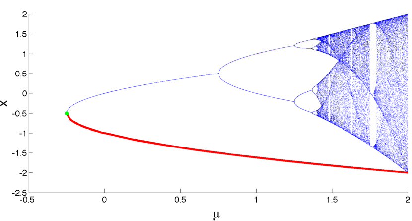
Figure 1: Cascades for $F(\mu,x)=\mu-x^{2}$. This figure shows the attracting set for $F$ for $-0.25<\mu<2$. The attracting set is created at a saddle-node bifurcation at $\mu=-0.25$ (green dot). The path of unstable fixed points (red) exists for all $\mu>-0.25$. The stable fixed point undergoes infinitely many period-doubling bifurcations, limiting to the value $\mu\approx 1.4$. This set of period doublings is called a period-doubling cascade. This map also has infinitely many period-doubling cascades that begin with periodic orbits of period $>1$. The red curve consists of unstable regular fixed points that exist for all $\mu>-0.25$.

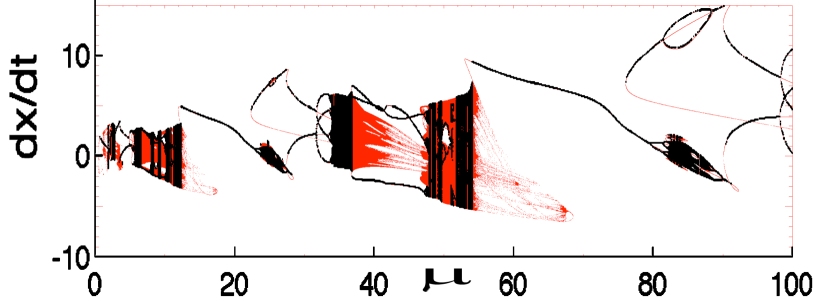
Figure 2: Cascades in the double-well Duffing equation. The attracting sets (in black) and periodic orbits up to period ten (in red) for the time-$2\pi$ map of the double-well Duffing equation: $x^{\prime\prime}(t)+0.3x^{\prime}(t)-x(t)+(x(t))^{2}+(x(t))^{3}=\mu\sin t$. Numerical studies show regions of chaos interspersed with regions without chaos, as in the Off-On-Off Chaos Theorem (Theorem 5).

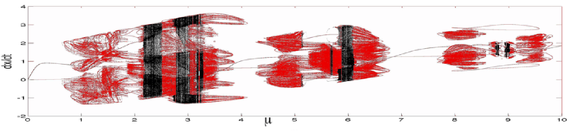
Figure 3: The forced-damped pendulum. For this figure, periodic points with periods up to ten were plotted in red for the time-$2\pi$ map of the forced-damped pendulum equation: $x^{\prime\prime}(t)+0.2x^{\prime}(t)+\sin(x(t))=\mu\cos(t)$, indicating the general areas with chaotic dynamics for this map. Then the attracting sets were plotted in black, hiding some periodic points. Parameter ranges with and without chaos are interspersed.

In Figure  1, as $\mu$ increases from $\mu=-0.25$ towards a value $\mu_{F}\approx 1.4$, a family of periodic orbits undergoes an infinite sequence of period doublings with the periods of these orbits tending to $\infty$. This infinite process is called a cascade. We will later define it more precisely. It has been repeatedly observed in a large variety of scientific contexts that the presence of infinitely many period-doubling cascades is a precursor to the onset of chaos. For example, cascades occur in what numerically appears as the onset to chaos for both the double-well Duffing equation, as shown Figure 2, and the forced-damped pendulum, shown Figure 3. Cascades were first reported by Myrberg in 1962 [9], and studied in more detail by Feigenbaum [4]. This cascade is not the only cascade. In fact, there are infinitely many distinct period-doubling cascades. Namely, there are infinitely many windows, that is, disjoint intervals in the parameter that begin with a saddle-node (or source-sink) bifurcation, and continue with the attractor undergoing an infinite sequence of period doublings within that interval of parameters.

Quadratic maps as in the example in Figure  1 has the quite atypical property that as the parameter increases, there are no bifurcations that destroy periodic orbits. Such maps are called monotonic. (This monotonicity was originally proved implicitly by Douady and Hubbard in the complex analytic setting. See the Milnor-Thurston paper [7] for a proof.) Once one knows that a map is monotonic, it is easy to show that as chaos develops there must be infinitely many cascades. See Figures  1, and 4–8.

The monotonicity property is a quite severe restriction, even in one-dimension. No higher dimensional maps that develop chaos are monotonic; yet numerical studies indicate that there are infinitely many cascades whenever there is one. See for example Figures 2, 3, and 5. In this paper we summarize our progress and give new extensions to our theory that explains why there are infinitely many cascades in the onset to chaos. Our explanation is also valid for maps of arbitrary dimension.

In the first result of this paper, we consider the context in which virtually all periodic saddles have the same unstable dimension. (By virtually we mean all except for a finite number.) In this case, the onset of chaotic behavior always includes infinitely many cascades.

There is an extensive literature on Routes to Chaos; that is, situations in which for some $\mu_{1}$ and $\mu_{2}$, the trajectory of $x$ under $F(\mu_{2},\cdot)$ is in the basin of a chaotic attractor, whereas under $F(\mu_{1},\cdot)$ it is not. Whatever might have happened that caused this change between $\mu_{1}$ and $\mu_{2}$ is called a route to chaos. We prefer to call these “routes to a chaotic attractor” to be more specific. There are many different routes to a chaotic attractor. See our discussion section for a partial enumeration. For many maps there is competition between instability and stability. For example, the appearance of an attracting periodic orbit as a parameter is varied may mask the chaotic dynamics, and when the orbit becomes unstable, a chaotic attractor is likely to appear. Hence a periodic orbit’s loss of stability is one example of a route to a chaotic attractor. This approach ignores the question we address here: how did the chaotic dynamics arise in the first place?

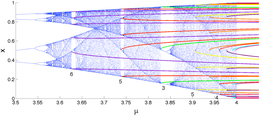
Figure 4: Cascades for $F(\mu,x)=\mu x(1-x)$. The logistic map has infinitely many cascades of attracting periodic orbits, and all cascades start at the stable orbit of a saddle-node bifurcation. The unstable orbits form what we call the stems of the cascades (shown in color). Each stem continues to exist for all large $\mu$ values. By our terminology, this means that all the cascades shown are solitary (on any parameter interval $[\mu_{1},\mu_{2}]$, for $\mu_{1}=3.5$ and any $\mu_{2}>4$) since the stem does not connect its cascade to a second cascade. The stems are shown here up to period six. Different colors are used for different periods.

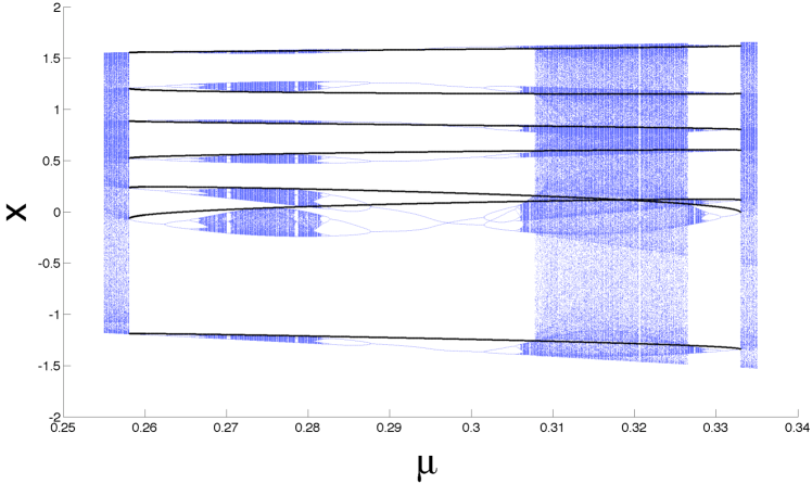
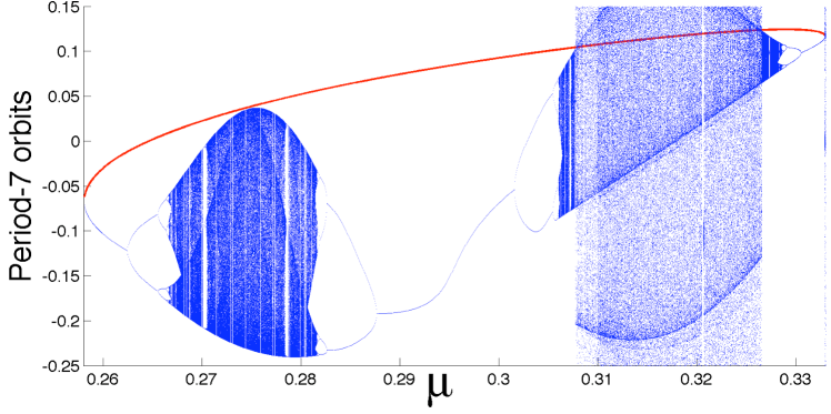
Figure 5: Paired cascades in the Hénon map $(u,v)\mapsto(1.25-u^{2}+\mu v,u)$. The top bifurcation diagram shows a set of four period-7 cascades. The bottom bifurcation diagram shows detail of the top part. Only one point of each of the period-7 orbits of the Hénon map are shown so that it is clearer how the two pairs connect to each other. The leftmost and rightmost cascades form a pair that is connected by a path of unstable regular periodic orbits (shown in red). Likewise, the two middle cascades form a pair. It is connected by a path of attracting period-seven orbits (blue). Paired cascades are not robust to moderate changes in the map.

Two types of cascades. For maps with the monotonicity property, each cascade is solitary, in that it is not connected to another cascade by a path of regular periodic orbits. These paths are the colored stems shown in Figure  4. See Section  2 for full definitions of these terms. Furthermore, the chaos persists for all parameters larger than a certain value. However, in many scientific contexts, it is common to see chaotic behavior appear and then disappear as the parameter $\mu$ increases. Thus as it increases there is both a route to chaos followed by a route away from chaos. In this situation virtually all cascades are paired; that is, two cascades are connected by a path of regular periodic orbits. See Figure  5.

Solitary cascades are robust. In our second set of results, we show that while paired cascades can be easily created and destroyed, solitary cascades are far more robust even in the presence of rather large perturbations of a map. Solitary cascades usually have stems with a constant period. This stem-period can be thought of as the period that starts the cascade. These ideas give quite striking results. For example for each period $p$ the following two maps

$$Q(\mu,x)=\mu-x^{2}$$

and

$$\widetilde{Q}(\mu,x)=\mu-x^{2}+1000\cos(\mu^{3}+x)$$

have exactly the same number of solitary cascades of stem-period $p$ – assuming the bifurcations of the second map are generic. Namely, we call a map generic if its periodic orbit bifurcations are all generic. See Section 2 for the full definitions of these terms. We know that all the bifurcation orbits are generic for almost every smooth map, and that if a smooth map is not generic, then it has infinitely many generic maps arbitrarily close to it, but unfortunately – with few exceptions – we cannot tell if a given map is generic.

The map $Q$ has no paired cascades, but the $\widetilde{Q}$ may. For example there is exactly one solitary cascade with stem-period $1$ and one with stem-period $3$. These results extend to

$$F(\mu,x)=\mu-x^{2}+g(\mu,x)$$

where g is smooth (ie. infinitely continuously differentiable) and $|g(\mu,x)|$ and $|g_{x}(\mu,x)|$ are uniformly bounded – as would be the case if $g$ was smooth and periodic in each variable, again assuming the map $F$ has generic bifurcations.

Outline. The paper proceeds as follows: In Section 2, we give some basic definitions, including what we mean by a cascade, the definition of chaos that we use here, and the class of generic maps with which we work. Section 3 contains a series of results relating chaos and cascades, with an explanation of the concrete relationship between periodic orbits within the chaos and the resulting cascades along the route towards this chaos. In Section 4, we discuss the fact that all cascades are either paired or solitary, and show that solitary cascades are robust under changes in the map.

In Section 5, we show that if there is chaotic behavior interspersed with non-chaotic behavior, then virtually all cascades are paired. It is common in scientific applications that chaos is interspersed with orderly behavior, in what we call off-on-off chaos (defined formally in Section 5). Our numerical studies indicate that this occurs multiple times for both the forced-damped pendulum and double-well Duffing examples.

We end with a discussion and present open questions in Section 6.

2 Definitions

Figure 6: Center manifold of saddle-node bifurcations and period-doubling bifurcations. This figure shows typical saddle-node and period-doubling (halving) bifurcations, along with the stability. For generic maps $F:R\times R^{n}$, it is sufficient to examine the $R\times R$ center manifold. We plot one-dimensional $x$ vertically and $\mu$ horizontally. We use vertical arrows to show how the stability varies near a bifurcation periodic point – indicated by a large dot. In each case, all the stability arrows can be reversed, thereby generating four more cases.

Figure 7: The regular periodic orbits form a one-manifold near regular saddle-node and period-doubling bifurcation orbits. In this schematic figure each point is an orbit and the horizontal axis is the parameter, usually $\mu$ in this paper. (a & b): Near a standard saddle-node bifurcation of a periodic orbit, the local invariant set consists of a curve of periodic orbits. They are either all flip orbits or all regular periodic orbits. Therefore RPO is locally a curve. (c & d): Near a standard period-doubling (or period-halving) bifurcation of a periodic orbit, the local invariant set consists of two curves of periodic orbits, one of period $p$ shown as segment AB, and one of period $2p$ shown as segment C. Segment C always consists of regular periodic orbits, whereas exactly one of A and B consists of flip orbits and the other regular periodic orbits. Thus RPO is locally a curve consisting of C and either A or B, depending on which is regular. For the quadratic map $\mu-x^{2}$, only (a) and (d) occur. That is, periodic orbits are created but never destroyed as $\mu$ increases. When $x$ is two-dimensional, such simplicity virtually never occurs [5].

Figure 8: A depiction of a monotonic cascade. A cascade is a path of regular periodic orbits that has infinitely many period-doubling bifurcations with the periods going to infinity at the end of the path. Solid lines denote regular orbits, and dashed lines denote flip orbits. This figure uses only the orbit-creation bifurcations, (a) and (d) in Figure 7. If only bifurcation types (a) and (d) are present and $x$ is scalar, then each saddle-node spawns an unstable branch and an attractor as $\mu$ increases. For $\mu-x^{2}$, there are no attractors for $\mu>\mu_{2}$ for $\mu_{2}$ sufficiently large. Hence this branch of attractors cannot continue forever and must bifurcate. Only (d) is available, spawning a flip orbit branch and a doubled-period branch of attractors. Again this new branch of attractors cannot continue forever as $\mu$ increases. In this way, an infinite set of period-doublings results before $\mu$ reaches $\mu_{2}$. Much more complicated patterns are possible when all four types of bifurcations are allowed, including period-halving as well as period-doubling, and the path may contain many saddle-node bifurcations.

We investigate smooth maps $F(\mu,x)$ where $\mu$ is in an interval $J$, and $x$ is in a smooth manifold $\mathfrak{M}$ of any finite dimension. For example, for the forced damped pendulum,

$$\frac{d^{2}\theta}{dt^{2}}+A\frac{d\theta}{dt}+\sin\theta=\mu\cos t,$$

we take $F(\mu,x)$ to be the time-$T$ map, where $T=2\pi$ is the period of the forcing, and $x=(\theta,d\theta/dt)$. Then the first coordinate of $x$ is on a circle, and the second is a real number. Hence $\mathfrak{M}$ is a cylinder.

We say a point $(\mu,x_{0})$ is a period-$p$ point if $F^{p}(\mu,x_{0})=x_{0}$ and $p$ is the smallest positive integer for which that is true. Its orbit, sometimes written $[(\mu,x_{0})]$, is the set

$$\{(\mu,x_{0}),(\mu,x_{1}),\cdots,(\mu,x_{p-1})\},\mbox{ where }x_{j}=F^{j}(\mu,x_{0}).$$

By the eigenvalues of a period-$p$ point $(\mu,x_{0})$, we mean the eigenvalues of the Jacobian matrix $D_{x}F^{p}(\mu,x_{0})$.

An orbit is called hyperbolic if none of its eigenvalues has absolute value 1. All other orbits are bifurcation orbits. Figure 6 depicts two standard examples of bifurcation orbits and the resulting stability of nearby periodic points.

We call a periodic orbit a flip orbit if the orbit has an odd number of eigenvalues less than -1, and -1 is not an eigenvalue. (In one dimension, this condition is: derivative with respect to $x$ is $<-1$. In dimension two, flip orbits are those with exactly one eigenvalue $<-1$.) All other periodic orbits are called regular. For example, the periodic orbits of constant period switch between flip and regular orbits at a period-doubling bifurcation orbit since an eigenvalue crosses $-1$. See Figure 7. We write RPO for the set of regular periodic orbits.

For some $a,b\in R$ and $\psi\in[a,b)$, let $Y(\psi)=(\mu(\psi),x(\psi))$ be a path of regular periodic points depending continuously on $\psi$. Assume $\psi$ does not retrace any orbits. That is, each $Y(\psi)$ is a periodic point on a regular periodic orbit, and distinct values of $\psi$ correspond to periodic points on distinct orbits. We call a regular path $Y(\psi)$ a cascade if the path contains infinitely many period-doubling bifurcations, and for some period $p$, the periods of the points in the path are precisely $p,2p,4p,8p,\dots$. As one traverses the cascade, the periods need not increase monotonically, but as $\psi\to b$, the period of $Y(\psi)$ goes to $\infty$. The orbits of a cascade with monotonic period increase are depicted schematically in Figure 8.

Write $fixed(\mu,p)$ for the set of fixed points of $F^{p}(\mu,\cdot)$ and $|fixed(\mu,p)|$ for the number of those fixed points. We say that there is exponential periodic orbit growth at $\mu$ if there is a number $G>1$ for which the number of periodic orbits of period p satisfies $|fixed(\mu,p)|\geq G^{p}$ for infinitely many $p$. For example, this inequality might hold for all even $p$, but for odd $p$ there might be no periodic orbits. This is equivalent to the statement that for some $h(=\log G)>0$, we have

$$\mbox{limsup}_{p\to\infty}\frac{\log|fixed(\mu,p)|}{p}\geq h.$$ (1)

Periodic orbit chaos. Chaotic behavior is a real world phenomenon, and trying to give it a single definition is like trying to define what a horse is. Definitions are imperfect. A child’s definition of a horse might be clear but would be unsatisfactory for a geneticist (whose definition might be in terms of DNA) and neither would satisfy a breeder of horses who might give a recursive definition, “an offspring of two horses.” Definitions of real-life phenomena describe aspects of that phenomena. They might agree in the great majority of cases on which animals are horses, though there may be rare atypical exceptions like clones where they might disagree. Just as it is impossible currently to connect the shape and sound of a horse with its DNA sequence, it is similarly impossible currently to identify in full generality positive Lyapunov exponents with exponential growth of periodic orbits.

Similarly “chaos” and “chaotic” should have definitions appropriate to the needs of the user. On the other hand, an experimenter might insist that to be chaotic, there must be a chaotic attractor, until he/she starts looking for chaos on basin boundaries and finds transient chaos. That approach leaves no terms for the chaos that occurs outside an attractor, as on fractal basin boundaries. We make no such restriction. Our results involve periodic orbits, and we make our definition accordingly.

We say a map $F(\mu,\cdot)$ has periodic orbit (PO) chaos at a parameter $\mu$ if there is exponential periodic orbit growth. This occurs whenever there is a horseshoe for some iterate of the map. It is sufficiently general to include having one or multiple co-existing chaotic attractors, as well as the case of transient chaos. As hinted at by Equation 1, in many cases PO chaos is equivalent to positive topological entropy. We discuss this relationship further in Section 6.

The unstable dimension Dim${}_{u}(\mu,x_{0})$ of a periodic point $(\mu,x_{0})$ or periodic orbit is defined to be the number of its eigenvalues $\lambda$ having $|\lambda|>1$, counting multiplicities.

We say there is virtually uniform (PO) chaos at $\mu$ if there is PO chaos, and all but a finite number of periodic orbits have the same unstable dimension, denoted Dim${}_{u}(\mu)$.

For the pendulum map discussed above, whenever there is PO chaos at some parameter value $\mu$, we expect the periodic orbits to be primarily saddles, and if it likewise had virtually uniform PO chaos, then we would expect $Dim_{u}(\mu)=1$. Assuming there are infinitely many periodic orbits, roughly half would be regular saddles, with the rest being flip saddles. Furthermore, all attracting periodic points are regular.

Our first goal is to describe the route to (PO) chaos. That is, if at $\mu_{1}$ there is no chaos, while at $\mu_{2}$ there is virtually uniform chaos, we explain what must happen in this interval in order for chaos to arise.

We believe that generally there is one typical route to chaotic dynamics. Namely, there must be infinitely many period-doubling cascades when $\mu$ is between $\mu_{1}$ and $\mu_{2}$. (Each of these cascades in turn has infinitely many period-doubling bifurcations.)

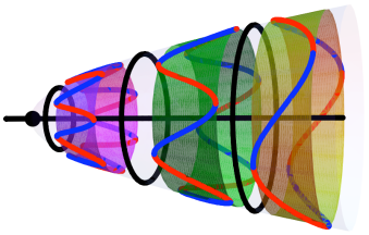
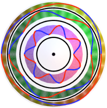
Figure 9: A regular periodic Hopf bifurcation point is locally contained in a unique curve of regular periodic orbits. To understand generic Hopf bifurcations, it is sufficient to determine the dynamics on its (invariant) center manifold, which is locally like $R^{2}\times R$. It contains all periodic orbits that are near the bifurcation orbit. Near a generic Hopf bifurcation with no eigenvalues which are roots of unity, the local invariant set consists of a curve of periodic points (in solid black) and a surrounding paraboloid (at left). Although there are infinitely many periodic orbits on the paraboloid in each neighborhood of the Hopf bifurcation point, the middle curve of periodic points is disconnected from all periodic points on the paraboloid. Specifically, the paraboloid contains infinitely many annuli converging to the bifurcation point, each with periodic orbits formed and destroyed at saddle-node bifurcations. Typical annuli are depicted here by colored regions. The periodic orbits are depicted in blue (saddles) and red (nodes). Between every two annuli, there is an invariant circle (in black) with irrational rotation number, as made clear by the projection (at right) of the paraboloid to the center manifold plane of the phase space.

Generic maps. Our results are given for generic maps of a parameter. Specifically, we say that the map $F$ is generic if all of the bifurcation orbits are generic, meaning that each bifurcation orbit is one of the following three types:

1. A standard saddle-node bifurcation. (Where “standard” means the form of the bifurcation stated in a standard textbook, such as Robinson [11].) In particular the orbit has only one eigenvalue $\lambda$ for which $|\lambda|=1$, namely $\lambda=1$.

2. A standard period-doubling bifurcation. In particular the orbit has only one eigenvalue $\lambda$ for which $|\lambda|=1$, namely $\lambda=-1$.

3. A standard Hopf bifurcation. In particular the orbit has only one complex pair of eigenvalues $\lambda$ for which $|\lambda|=1$. We require that these eigenvalues are not roots of unity; that is, there is no integer $k>0$ for which $\lambda^{k}=1$.

These three bifurcations are depicted in Figures 7 and 9. Generic $F$ have at most a countable number of bifurcation orbits, so almost every $\mu$ has no bifurcation orbits. See [13] for the details showing that these maps are indeed generic in the class of smooth one-parameter families. For systems with symmetry such as the forced-damped pendulum, a fourth type of bifurcation occurs, such as a pitchfork or symmetry-breaking bifurcation. This adds complications, though in fact with extra work our results remain true.

Our motivation for considering generic maps is given in Proposition 1 in the next section, which states that each regular periodic orbit for a generic map is locally contained in a unique path of periodic orbits. The connection to cascades can be summarized as follows: starting at each regular periodic orbit $Q$ for $\mu\in[\mu_{1},\mu_{2}]$, there is a local path of regular periodic orbits through $Q$. Enlarge this path as far as possible. Either the path reaches $\mu_{1}$ or $\mu_{2}$, or there is a cascade. This idea is explained in more detail in the next section.

3 Onset of chaos implies cascades

Our first result is Theorem 1, which demonstrates that the route to virtually uniform PO chaos contains infinitely many period-doubling cascades. Theorem 2 is a restatement of these results in a way that makes the relationship between chaos and cascades much more transparent.

Write $J$ for the closed parameter interval $[\mu_{1},\mu_{2}]$. Our main hypotheses will be used for a variety of results so we state them here.

List of Assumptions.

1. Assume $F$ is a generic smooth map; that is, $F$ is infinitely differentiable in $\mu$ and $x$, and all of its bifurcation orbits are generic.

2. Assume there is a bounded set $M$ that contains all periodic points $(\mu,x)$ for $\mu\in J$.

3. Assume all periodic orbits at $\mu_{1}$ and $\mu_{2}$ are hyperbolic.

4. Assume that the number $\Lambda_{1}$ of periodic orbits at $\mu_{1}$ is finite.

5. Assume at $\mu_{2}$ there is virtually uniform PO chaos. Write $\Lambda_{2}$ for the number of periodic orbits at $\mu_{2}$ having unstable dimension not equal to Dim${}_{u}(\mu_{2})$.

Theorem 1.

Assume ($A_{0}~{}-~{}A_{4}$). Then there are infinitely many distinct period-doubling cascades between $\mu_{1}$ and $\mu_{2}$.

Example 1.

Based on numerical studies, a number of maps appear to satisfy the conditions of the above theorem. Note that numerical verification involves significantly more work than just plotting the attracting sets for each parameter, since we are concerned about both the stable and the unstable behavior to determine whether there is chaos. Examples include the time-$2\pi$ maps for the double-well Duffing (Fig. 2), the triple-well Duffing, the forced-damped pendulum (Fig. 3), the Ikeda map (introduced to describe the field of a laser cavity), and the pulsed damped rotor map.

This formulation gives no idea how the behavior at $\mu_{2}$ is connected to the cascades that must exist. Thus before giving a proof, we reformulate the conclusions of the theorem in a more transparent way. Specifically, we reformulate so that it is clear how infinitely many cascades in the strip $S=[\mu_{1},\mu_{2}]\times\mathfrak{M}$ are connected to regular periodic orbits at $\mu_{2}$ by continuous paths in RPO.

Paths of orbits. We now give a formal definition for paths of regular periodic orbits and show that they connect regular periodic orbits at $\mu_{2}$ with cascades between $\mu_{1}$ and $\mu_{2}$. We start with the following theorem, which guarantees that a path through each regular periodic orbit is unique.

Assume hypotheses $A_{0}-A_{4}$, and consider a local path through a regular periodic orbit as guaranteed by the above proposition. Specifically, let $Y_{0}=(\mu_{2},x_{0})$ be a regular periodic point. Since all such points at $\mu_{2}$ in the above theorem are assumed to be hyperbolic, the orbit can be followed without a change of direction for nearby $\mu<\mu_{2}$. We can define $Y(\psi)=(\mu(\psi),x(\psi))$ continuously for $\psi$ in an interval $[\psi_{0},\psi_{1}]$ as follows. Let $Y(\psi_{0})=(\mu_{2},x_{0})$. Then $Y(\psi)$ follows the branch of regular periodic points for decreasing $\mu$ until reaching $Y(\psi_{1})$, which is either a bifurcation orbit or $\mu=\mu_{1}$. If it is a bifurcation point, which would be a generic bifurcation point, then from the above proposition there is a unique branch of regular hyperbolic periodic points leading away from $Y(\psi_{1})$, and $Y(\psi)$ follows that branch. If $Y(\psi_{1})$ is a period-doubling bifurcation point, there are two branches of regular periodic points, but both are on the same orbits. Either branch can be followed since both represent the same orbits and both are regular.

Each branch of hyperbolic periodic orbits can be parametrized by $\mu$ and is easy to find numerically by solving a differential equation. Write $A(\mu)$ for the square matrix $D_{x}F^{p}(\mu,x(\mu))$ and $b(\mu)$ for the vector $D_{\mu}F^{p}(\mu,x(\mu))$. Differentiating

$$F^{p}(\mu,x(\mu))=x(\mu)$$

with respect to $\mu$ and manipulating yields

$$b(\mu)+A(\mu)\frac{dx}{d\mu}=\frac{dx}{d\mu},\mbox{ or }$$

$$\frac{dx}{d\mu}=-(A(\mu)-Id)^{-1}\;b(\mu),$$

Where $Id$ denotes the identity matrix. The matrix inverse above exists since $(\mu,x(\mu))$, being hyperbolic, cannot have $+1$ as an eigenvalue.

This construction suggests a definition. We say $Y(\psi)$ is a path in $S$ for $\psi$ in some interval $K$ if it is continuous and

• $Y(\psi)$ is a regular periodic point in $S$ for each $\psi\in K$;

• Y does not retrace orbits; that is, $Y$ is never on the same orbit for different $\psi$.

Proposition 1 (Local paths of regular periodic points).

For a smooth generic map $F:R\times{\mathfrak{M}}\to{\mathfrak{M}}$, each regular periodic point is locally contained in a path of regular periodic points. The corresponding path of periodic orbits is unique.

This proposition appears in reference [13]. Here we give an idea of the proof. The implicit function theorem shows that there is a local curve of periodic points through a regular hyperbolic periodic point. Therefore, the proof consists of showing that there is also a local curve of orbits through each periodic bifurcation orbit. This must be shown for each of the three types of generic bifurcations. The curve is not necessarily monotonic: It may reverse direction with respect to $\mu$, as depicted in Figure 6. Namely, a path $Y(\psi)=(\mu(\psi),x(\psi))$ reverses direction at $\psi_{0}$ if $\mu(\psi)$ changes from increasing to decreasing or vice versa at that point. For n-dimensional $x$, the study of generic saddle-node and period-doubling bifurcations can be reduced to one-dimensional $x$ due to the center manifold theorem. The bifurcation orbit has $n-1$ eigenvalues outside the unit circle, and these do not affect the dynamics on the two-dimensional invariant $(\mu,x)$-plane. Hence here we can consider $x$ as being one-dimensional.

In the case of a saddle-node bifurcation, one branch of orbits is stable and one is unstable in $R^{1}$. Since the other $n-1$ eigenvalues do not cross the unit circle near the point, it follows that the unstable dimension of the orbits in $n-$dimensions is even for one branch and odd for the other, i.e., the unstable dimension $k(\psi)$ of $Y(\psi)$ changes parity as $Y(\psi)$ passes through the bifurcation point $Y(\psi_{0})$.

For a period-doubling bifurcation, consider the notation depicted in Figure 6. Namely, let (A) denote the period-$n$ orbits with no coexisting period-$2n$ orbits, let (B) denote the branch of period-$n$ orbits coexisting at the same parameter values with the branch (C) of period-$2n$ orbits. If branch (A) is regular and (B) is flip, then the path $Y$ includes branches (A) and (C), which are on different sides of the bifurcation point, and $\mu(\psi)$ does not change direction and $k(\psi)$ does not change parity. If however (B) is regular and (A) is flip, then $\mu(\psi)$ does change direction and $k(\psi)$ does change parity.

For Hopf bifurcations (see Figure 9), the path proceeds monotonically past the bifurcation point and the unstable dimension changes by $\pm 2$, so the parity does not change. Hence in all cases, the path changes direction if and only if the parity changes. The cases of saddle-node and period-doubling bifurcations are straightforward, as depicted in Figure 7. To show that RPO is locally a curve at a Hopf bifurcation is trickier than the other two cases, since there are in fact infinitely-many periodic orbits near a Hopf bifurcation point, but they are not connected to the Hopf bifurcation point by any path of periodic points, as shown in Figure 9. The proof follows from the steps listed.

Cascades. We call a regular path $Y(\psi)$ for $\psi\in[a,b)$ a cascade if the path contains infinitely many period-doubling bifurcations, and for some period p, the periods of the points in the path are precisely $p,2p,4p,8p,\cdots$. As one traverses the cascade, the periods need not increase monotonically, but as $\psi\to b$, the period of $Y(\psi)$ goes to $\infty$.

We will say a path $Y(\psi)$ is maximal if the following additional condition holds:

• $Y$ cannot be extended further to a larger interval, and it cannot be redefined to include points of more regular orbits.

Figure 10 shows an example of a middle portion of a maximal path. Figure 11 and 12 show different possibilities for how the maximal path ends.

Figure 10: Paths of regular periodic orbits. We assume here that all bifurcation orbits are generic. It follows that a regular periodic point is in a path of periodic points. Since each periodic point is in a periodic orbit, we can think of the path as being a path of regular periodic orbits. This is a unique path of regular orbits (solid). Here we show orbits, not points. Flip orbits are depicted by dashed lines, showing that the path is no longer unique if we include all periodic orbits. Let $Y(\psi)$ be a path of regular (non-flip) periodic points parametrized by $\psi$, such that $Y(\psi)$ does not pass through the same orbit twice. Write $[Y(\psi)]$ for the orbit that the point $Y(\psi)$ is in. It is a useful fact that whenever the $\mu$ coordinate $\mu(\psi)$ of $Y(\psi)$ changes direction, the unstable dimension of $Y(\psi)$ changes by one. Hence it changes from odd to even or vice versa. The arrows along the path show which way the path is traveling as $\psi$ increases.

Figure 11: Paths of regular periodic orbits starting from $\mu_{2}$. Assume the bifurcations are generic. We use the notation of the above figure. Let $Y_{0}=(\mu_{2},x_{0})$ be a regular hyperbolic periodic point. If its maximal path of orbits extends to a hyperbolic orbit $Y_{0}^{*}$ at $\mu_{1}$, then the path has changed directions an even number of times and the unstable dimensions of $Y_{0}$ and $Y_{0}^{*}$ have the same parity; that is, both are even or both are odd. If the path starting at a regular hyperbolic orbit $Y_{1}=(\mu_{2},x_{1})$ returns to a point $Y_{1}^{*}$ at $\mu_{2}$, the path changes directions an odd number of times, and so the unstable dimensions of $Y_{1}$ and $Y_{1}^{*}$ have opposite parity and in particular the unstable dimensions of the two are different.

Figure 12: An interior path of regular orbits starting from $\mu_{2}$ yields cascades. Continuing the assumptions and notations of the above figures, assume the hypotheses of Theorem 1. Only a finite number of paths that start at $\mu_{2}$ can either reach $\mu_{1}$ or return to $\mu_{2}$. Hence there are an infinite number of regular hyperbolic orbits at $\mu_{2}$ that yield paths that neither reach $\mu_{1}$ nor return to $\mu_{2}$. Such interior paths must contain an infinite number of bifurcations. Since generically there are only a finite number of bifurcation orbits of each period between $\mu_{1}$ and $\mu_{2}$, the period of the orbits must tend to infinity along the path and it must contain a cascade. Hence there are infinitely many cascades between $\mu_{1}$ and $\mu_{2}$.

Let Orbits(Y) be the set of periodic points on orbits traversed by $Y$. That is, if $(\mu,x)=Y(\psi)$ for some $\psi$, then $(\mu,x)\in\mbox{Orbits}(Y)$ and so are the other points on the orbit, $(\mu,F^{n}(\mu,x))$ for all n.

Two integers are said to have the same parity if both are odd or both are even. Otherwise they have opposite parity. Figures 6 and 10 demonstrate why this is a critical idea. Namely, the unstable dimension of a path $Y(\psi)$ changes parity as $\psi$ increases precisely when the path changes directions. Thus the parity of the unstable dimension corresponds to the orientation of the path.

Theorem 2.

Assume ($A_{0}~{}-~{}A_{4}$). Then the following are true.

• there are infinitely many regular periodic points at $\mu_{2}$.

• For each maximal path $Y(\psi)=(\mu(\psi),x(\psi))$ in $S$ starting from a regular periodic point $Y_{0}=(\mu_{2},x_{0})$, the set of orbits traversed, denoted by Orbits$(Y)$, depends only on the initial orbit containing $Y_{0}$. That is, different initial points on the same orbit yield paths that traverse the same set of orbits, so we can write Orbits$(Y_{0})$ for Orbits$(Y)$.

• Let $Y_{0}=(\mu_{2},x_{0})$ and $Y_{1}=(\mu_{2},x_{1})$ be regular periodic points on different orbits. Then Orbits$(Y_{0})$ and Orbits$(Y_{1})$ are disjoint.

• Let $K$ denote the unstable dimension of a regular periodic point $(\mu_{2},x_{0})$. For a maximal path $Y(\psi)=(\mu(\psi),x(\psi))$ in $S$ starting from $(\mu_{2},x_{0})$, let $k(\psi)$ denote the unstable dimension of $Y(\psi)$. At each direction-reversing bifurcation, $k(\psi)$ changes parity; that is it changes from odd to even or vice versa. Initially $Y(a)=(\mu_{2},x_{0})$ so initially $\mu(\psi)$ is decreasing and $k(a)=K$, so initially $k(a)+K$ is even. Hence in general $\mu(\psi)$ is decreasing if $K+k(\psi)$ is even and increasing if it is odd.

• Let $Y$ be a maximal path on $[a,b]$ in $S$ and $\mu(a)=\mu_{2}$. If $\mu(b)=\mu_{2}$, then $\mu(\psi)$ is increasing at that point so $k(a)+k(b)$ is even. Hence $k(a)+k(b)$ is odd, so $k(a)\neq k(b)$.

• There are infinitely many distinct period-doubling cascades between $\mu_{1}$ and $\mu_{2}$.

• There are at most $\Lambda=\Lambda_{1}+\Lambda_{2}$ regular periodic orbits at $\mu_{2}$ with unstable dimension Dim${}_{u}(\mu_{2})$ that are not connected to cascades.

Theorem 2 is a version of Theorem 1 that allows us to show that most regular orbits at $\mu_{2}$ are connected to cascade by a path of regular orbits. The conclusions of this theorem were shown to hold in [13] under assumptions $A_{0}-A_{4}$ along with the additional hypothesis that at $\mu_{2}$, there are infinitely many periodic regular orbits. However, we are now able to show that this last hypothesis is unnecessary because it is automatically true. In fact, under assumptions $A_{0}-A_{4}$, approximately half of the periodic orbits are regular. This proof is quite technical in that it involves topological fixed point index theory. To make this treatment more readable, we give the full details in [14].

Example 2.

Assume phase space is two-dimensional. If at $\mu_{2}$ there is a transverse homoclinic point then there will be infinitely many saddles and exponential orbit growth. Condition $A_{2}$ is often satisfied if the attractor(s) are periodic orbits and there is a Smale horseshoe in the dynamics.

Example 3.

Our numerical studies of the forced-damped pendulum indicate that it satisfies the hypotheses of this theorem on $[\mu_{1},\mu_{2}]\approx[1.8,20],[73,20],[73,175],$ and $[350,175]$. Thus there are infinitely-many cascades on each of these intervals.

Weakening the uniformity hypothesis. We end this section with the conjecture that $A_{4}$ can be weakened without effecting the conclusions of the theorem. Specifically, let $\Phi(\mu,K,p)$ be the fraction of all period-p orbits at $\mu$ that have unstable dimension $K$. We will say that most periodic orbits have unstable dimension $K$ if $\Phi(\mu,K,p)\to 1$ as $p\to\infty$. We believe that for most generic smooth maps and most $\mu$, there is some dimension $u_{0}$ for which this holds.

Conjecture 1.

Assume ($A_{0}~{}-~{}A_{3}$) (not including ($A_{4}$)). Assume that most periodic orbits at $\mu_{2}$ have unstable dimension $K$. Then there are infinitely many regular periodic orbits with unstable dimension $K$, and infinitely many of these are connected to distinct period-doubling cascades between $\mu_{1}$ and $\mu_{2}$.

4 Conservation of solitary cascades

Let $J$ be an interval, and let $Y(\psi)$ for $\psi\in J$ be a maximal path of regular periodic orbits containing a cascade. For any point $s_{0}$ in the interior of $J$, infinitely many period doublings of the cascade occur either for $\psi<s_{0}$ or $\psi>s_{0}$. In the following definition, we distinguish two types of cascades based on what happens to the other end of $Y(\psi)$.

Definition 1.

Let $F$ satisfy $A_{0}-A_{2}$. A cascade is solitary in $[\mu_{1},\mu_{2}]$ if the maximal path of regular periodic orbits containing it contains no other cascades. In this case, we call the non-cascade end of the maximal path the stem of the cascade. A cascade is paired if its maximal path contains two cascades. A cascade is bounded in $[\mu_{1},\mu_{2}]$ if its maximal path is contained in the interior of the interval and never hits the boundary $\mu=\mu_{1}$ or $\mu=\mu_{2}$. We call a path which stays in the interior of the interval an interior path.

On a sufficiently large parameter interval, all cascades for quadratic maps are solitary, as shown in Figure 4. Figure 5 shows an example of two sets of paired cascades. The following theorem shows that the classification of solitary versus paired is equivalent to classifying cascades in an interval as being purely interior versus hitting the interval boundary.

Theorem 3 (Solitary and paired cascades).

Let $F$ satisfy $A_{0}-A_{2}$ on $[\mu_{1},\mu_{2}]$. A cascade is paired if and only if the maximal path containing the cascade is an interior path. In particular, bounded cascades are always paired.

The maximal path of a solitary cascade contains a periodic point on the interval boundary; i.e. there is a point $(\mu,x)$ in the maximal path of the cascade such that $\mu=\mu_{1}$ or $\mu=\mu_{2}$. Namely, solitary cascades are never bounded.

Proof.

We give a sketch of the proof. Let $J$ be an interval, and let $Y(\psi)$ for $\psi\in J$ be a maximal path of regular periodic points in $[\mu_{1},\mu_{2}]$ containing a cascade as $\psi$ increases. Fix $s_{0}\in J$, and consider the one-sided maximal paths $Z_{\pm}(\psi)\subset Y(\psi)$ where $Z_{\pm}(\psi)=Y(\psi)$ respectively for $\psi>s_{0},\psi<s_{0}$, $\psi\in J$. We have assumed that $Z_{+}(\psi)$ contains the cascade. Therefore $Z_{+}(\psi)$ is an interior path, since otherwise there would not be infinitely many period-doubling bifurcations.

Key Fact: By the methods described in Section 3, a one-sided maximal path of regular periodic points is an interior path if and only if it contains a cascade.

Assume the cascade in $Y(\psi)$ is paired. Then $Z_{-}(\psi)\subset Y(\psi)$ contains a cascade, so by the key fact above, $Z_{-}(\psi)$ is an interior path, implying $Y(\psi)$ is as well.

Conversely, if $Y(\psi)$ is an interior path, then $Z_{-}(\psi)$ is as well, and by the key fact $Z_{-}(\psi)$ contains a cascade, meaning that the cascades in $Z_{\pm}(\psi)$ are paired. ∎

Conservation of solitary cascades. If $F$ satisfies $A_{0}-A_{4}$, and $\Lambda_{1}=\Lambda_{2}=0$, then Theorem 1 implies that there is conservation of solitary cascades. Specifically, let $\tilde{F}$ be any generic map such that $F$ and $\tilde{F}$ agree at $\mu_{1}$ and $\mu_{2}$, though they may have completely different behavior inside the interval. Then $F$ and $\tilde{F}$ have exactly the same solitary cascade structure. Since the number of cascades is infinite, this does not appear to be a meaningful statement. However, we can classify solitary cascades by looking at the period of their stems, and it is in this sense that their cascades are the same. In Figure 4 we label five solitary cascades, one of period three, one of period four, two of period five, and one of period six.

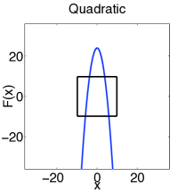
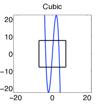
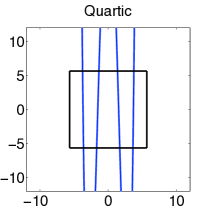
Figure 13: Quadratic, Cubic, and Quartic Maps. The three maps from Eqn. 2, are shown for $g=0$ and for $\mu=24,15,$ and $8$, respectively. The squares depicted are $[-2\sqrt{\mu},2\sqrt{\mu}]^{2}$. The maxima and minima are far larger than the size of the boxes, resulting in purely uniform chaotic behavior within the boxes. This is typical for large $\mu$. As $\mu$ increases, these three graphs would be stretched vertically. The values of the map $F$ for large $\mu$ at the critical points are proportional to $\mu$, $\mu^{3/2}$, and $\mu^{2}$, respectively, largely unaffected by $g$, which is bounded and has bounded derivative.

Three rigorous examples of conservation of solitary cascades are encapsulated in the following one-dimensional maps (see Figure 13):

$$F(\mu,x)=\mu-x^{2}+g(\mu,x) (\mbox{quadratic}),$$ (2)

$$F(\mu,x)=\mu x-x^{3}+g(\mu,x) (\mbox{cubic}),$$

$$F(\mu,x)=x^{4}-2\mu x^{2}+{\mu^{2}}/{2}+g(\mu,x) (\mbox{quartic}),$$

where $g$ is smooth, and for some real positive $\beta$,

$$|g(\mu,0)|<\beta \mbox{ for all }\mu,\mbox{ and }$$ (3)

$$|g_{x}(\mu,x)|<\beta \mbox{ for all }\mu,x.$$

It is straightforward to show that for $g\equiv 0$, each of these maps has a $[\mu^{*}_{1},\mu^{*}_{2}]$ such that there are no regular periodic orbits for $F$ at $\mu^{*}_{1}$, and $F$ has virtually uniform (PO) chaos at $\mu^{*}_{2}$. This leads to the fact that for $g$ of the form given, each of the three maps has no regular periodic orbits for $\mu_{1}$ sufficiently negative, and for $\mu_{2}$ sufficiently large has a one-dimensional horseshoe map. The conditions on $g$ guarantee that it does not significantly affect the periodic orbits when $|\mu|$ is sufficiently large; in particular it does not affect their eigenvalues, so it does not affect the number of period-$p$ regular periodic orbits for large $|\mu|$. Hence all three maps have no regular periodic orbits for $\mu$ small and have no attracting periodic orbits for $\mu$ large, and for sufficiently large $|\mu|$, all periodic orbits are contained in the set $[-2\sqrt{\mu},2\sqrt{\mu}]$. This leads to the following result:

Theorem 4 (Conservation of cascades).

For each of the functions $F$ in Eqn. 2, $F$ is generic for a residual set of $g$ chosen as in Eqn. 3. For each of the three examples, the number of stem-period-$k$ solitary cascades for all generic $F$ is independent of the choice of $g$.

In other words, fix $F$ to be one of the three types in Eqn. 2. Fix any $g$ as in Eqn. 3 such that $F$ is generic. Then there exist $\mu_{L}$ and $\mu_{M}$ such that as long as $\mu_{1}<\mu_{L}$ and $\mu_{2}>\mu_{M}$, $F$ has the same number of solitary cascades on $[\mu_{1},\mu_{2}]$ as occur in the $g\equiv 0$ case for the interval $[\mu^{*}_{1},\mu^{*}_{2}]$.

As an interpretation of this statement take a set $B$ as large as you like in parameter cross phase space, and make $g=-(\mu-x^{2})$ in $B$, so $F\equiv 0$ in $B$. Hence the only periodic orbit in $B$ is the fixed point $x=0$, so $B$ contains no cascades. It might seem that we have annihilated all cascades by this process, but the theorem guarantees that every single one of these solitary cascades will appear. They are just displaced from their original location, moved outside of $B$.

The conservation principle works for higher-dimensional maps as well. For example, we have shown in [12] that even large-scale perturbations of the two-dimensional Hénon map have conservation of solitary cascades. That is, writing $x=(x_{1},x_{2})$,

$$F(\mu,x_{1},x_{2})=\left(\begin{array}[]{c}\mu+\beta x_{2}-x_{1}^{2}+g(\mu,x_{1},x_{2})\\ x_{1}+h(\mu,x_{1},x_{2})\end{array}\right),\hskip 71.13188pt\mbox{(H\'{e}non)}$$

where $\beta$ is fixed, and the added function $(g,h)$ is smooth and is very small for $||(\mu,x_{1},x_{2})||$ sufficiently large. See [12] for a precise (and technical) formulation. Here the added terms cannot destroy the stems which are unchanged in the domain where $||(\mu,x_{1},x_{2})||$ is very large. Each stem must still lead to its own solitary cascade.

If $F(\mu,x_{1},\dots,x_{N})$ is a set of $N$ coupled quadratic maps such that

$$x_{i}\mapsto K(\mu)-x_{i}^{2}+g(x_{1},\dots,x_{N}),\hskip 71.13188pt\mbox{(coupled)}$$

where $g$ is bounded with bounded first derivatives, and $\lim_{k\to\pm\infty}K_{i}(\mu)=\pm\infty$, then there is conservation of solitary stem-period-$k$ cascades.

5 Off-on-off chaos for paired cascades

In the previous section, we concentrated on the implications of Theorem 3 on solitary cascades, but it also has implications for paired cascades. It describes a situation which is quite common in physical systems, namely the case in which parameter regions with and without chaos are interspersed, such as show in Figs. 2 and 3. Specifically, we give the following definition describing the situation where is no chaos at $\mu_{1}$ and $\mu_{3}$, while at $F$ is chaotic at $\mu_{2}$.

Definition 2 (Off-on-off chaos).

Assume $F$ satisfies $A_{1}$–$A_{4}$ on $[\mu_{1},\mu_{2}]$ and on $[\mu_{3},\mu_{2}]$, where $\mu_{1}<\mu_{2}<\mu_{3}$. Then $F$ is said to have off-on-off chaos for $\mu_{1}<\mu_{2}<\mu_{3}$.

If $F$ has off-on-off chaos, we can apply Theorem 2 to both $[\mu_{1},\mu_{2}]$ and to $[\mu_{2},\mu_{3}]$ and conclude that there are infinitely many cascades in each of the two intervals. The following theorem is stronger, in that we also conclude that virtually all regular periodic points at $\mu_{2}$ are contained in paired cascades.

Theorem 5 (Off-On-Off Chaos).

If $F$ has off-on-off chaos on $\mu_{1}<\mu_{2}<\mu_{3}$, then $F$ has infinitely many (bounded) paired cascades and at most finitely many solitary cascades in $(\mu_{1},\mu_{3})$.

The result follows directly from combining the results of Theorems 2 and 3.

Example 4.

Our numerical studies indicate that the time-$2\pi$ maps of the forced double-well Duffing (Fig. 2) and forced damped pendulum (Fig. 3) have off-on-off chaos, and that it occurs on multiple non-overlapping parameter regions. Here $2\pi$ is the forcing period. We cannot prove there are only finitely many periodic attractors, though we find very few. These systems have no periodic repellers.

6 Discussion

Our results in the context of routes to chaos. We now contrast our view with the traditional view of many different routes to chaos. People write about Routes to Chaos - where chaos does indeed mean there is a chaotic attractor. Below we list classes of distinct routes to chaotic attractors. Our results say that for generic smooth maps depending on a parameter, there is a unique route from no chaos to chaos (which we have defined to mean virtually uniform PO chaos) – in the sense of having a chaotic set that need not be attracting, for example when there is a transverse homoclinic point. Between a parameter value where there is no chaos and a parameter value where there is chaos, there must be infinitely many period-doubling cascades.

Routes to a chaotic attractor

1. A chaotic attractor develops where there was no previous horseshoe dynamics; this includes what we might call the Feigenbaum cascade route.

2. There is a transient chaos set and a simple non-chaotic attractor (equilibrium point or periodic orbit) and that attractor becomes unstable. For periodic orbits there are three ways to become unstable.

3. Like above except the attractor is a torus with quasiperiodic dynamics. How many ways can a torus become unstable? We suspect in many ways.

4. Crisis route: as a parameter decreases, a chaotic attractor collides with its basin boundary and the chaotic set is no longer attracting. How many ways can this happen? Also unknown.

5. There is a chaotic attractor and a non-chaotic attractor and as a parameter is varied, the initial condition being used migrates into the basin of the chaotic attractor.

6. Homoclinic explosions lead to chaotic dynamics.

However, using the viewpoint described in this paper, there is only one route to chaos.

Relating PO chaos and positive entropy. Consider the following definition, related to exponential growth of periodic orbits, alluded to when the definition was given: If $|fixed(p)|\sim G^{p}$ for large $p$, then we say $G$ is the growth factor, or we call $\log G$ the periodic orbit entropy. Taking logs of both sides, dividing by $p$, and taking limits, we get

$$\mbox{limsup}_{p\to\infty}\frac{\log|fixed(p)|}{p}=\log G=h.$$

We believe that many of the methods used here will lead to a fruitful study of periodic orbit entropy. Note that PO chaos occurs exactly when $h>0$. If there are only finitely many orbits for example, $h=0$. If there is at most a fixed number $k$ of periodic orbits of each period $p$, again $h=0$, even if there may be infinitely many orbits. In many situations, there is a relationship between exponential periodic growth and positive topological entropy, and in fact in some cases periodic orbit entropy is equal to topological entropy. We elaborate below.

Bowen showed [1] that for Axiom A diffeomorphisms, you can find topological entropy exactly by looking at the growth rate for the number of period-$p$ orbits as $p$ goes to infinity. For Hénon-like maps, Wang and Young proved that the topological entropy coincides with the exponential growth rate of the number of periodic points of period $p$ [15]. Chung and Hirayama [3] show that for any surface diffeomorphism with Hölder continuous derivative, the topological entropy is equal to the exponential growth rate of the number of hyperbolic periodic points of saddle type. That is, you can throw away the attractors and repellers.

In terms of interval maps: Misiurewicz and Szlenk [8] proved that if $f$ is a continuous and piecewise monotone map of the interval, then the topological entropy is bounded above by the exponential growth rate of the number of periodic orbits. Building on [6], Chung [2] showed that if $f$ is $C^{1+\alpha}$, similar results can be obtained if one counts only the set of hyperbolic periodic orbits (namely, periodic points $x$ for which $|(f^{p})^{\prime}(x)|^{1/p}>1$) or the set of transversal homoclinic points of a source.

Non-smooth maps. Continuous maps $F$ which are piecewise smooth but not smooth violate our assumptions, but such maps can be thought of as the limits of generic smooth maps $F_{n}$ which differ from $F$ only very near the discontinuities of $F_{x}$. In dimension one, $F=\mu+bx+c|x|$ gives a rich collection of examples obtained by choosing constants $b$ and $c$ in interesting ways. See the extensive literature on border collision bifurcations [10]. Such maps deserve more discussion than we can give here but we mention two examples.

(1) For the tent map $F(\mu,x)=\mu-2|x|$, there are no periodic orbits when $\mu<0$; there is one periodic orbit, a fixed point at 0, when $\mu=0$, and orbits of all periods when $\mu>0$. All orbits are in families of straight line rays that bifurcate from and originate at $(0,0)$, the map’s only bifurcation periodic orbit. In this case, all bifurcations in all the cascades that would exist for the approximating generic families $F_{n}$ tend to $(0,0)$ as $n\to\infty$.

(2) For the tent map with slope $\pm\mu$, namely $F(\mu,x)=1-\mu|x|$ for $1<\mu\leq 2$, a periodic orbit suddenly appears at $x=0$ for countably many $\mu$. For example if $\mu_{3}$ denotes the smallest parameter with a period-three orbit, then the point $x=0$ is a period-three point, and only infinitely many periodic orbits whose periods are multiples of three bifurcate from it. All of the cascades for those orbits that we would expect for a smooth map are collapsed into the single point $(\mu_{3},x=0)$.

References

- [1] R. Bowen. Topological entropy and axiom . In Global Analysis (Proc. Sympos. Pure Math., Vol. XIV, Berkeley, Calif., 1968), pages 23–41. Amer. Math. Soc., Providence, R.I., 1970.
- [2] Y. M. Chung. Topological entropy for differentiable maps of intervals. Osaka J. Math., 38(1):1–12, 2001.
- [3] Y. M. Chung and M. Hirayama. Topological entropy and periodic orbits of saddle type for surface diffeomorphisms. Hiroshima Math. J., 33(2):189–195, 2003.
- [4] M. J. Feigenbaum. The universal metric properties of nonlinear transformations. J. Statist. Phys., 21:669–706, 1979.
- [5] I. Kan, H. Kocak, and J. A. Yorke. Antimonotonicity: Concurrent creation and annihilation of periodic orbits. Annals of Mathematics, 136:219–252, 1992.
- [6] A. Katok and A. Mezhirov. Entropy and growth of expanding periodic orbits for one-dimensional maps. Fund. Math., 157(2-3):245–254, 1998. Dedicated to the memory of Wiesław Szlenk.
- [7] J. Milnor and W. Thurston. On iterated maps of the interval. In Dynamical systems (College Park, MD, 1986–87), volume 1342 of Lecture Notes in Math., pages 465–563. Springer, Berlin, 1988.
- [8] M. Misiurewicz and W. Szlenk. Entropy of piecewise monotone mappings. Studia Math., 67(1):45–63, 1980.
- [9] P. Myrberg. Sur l’itération des polynomes réels quadratiques. J. Math. Pures Appl. (9), 41:339–351, 1962.
- [10] H. E. Nusse, E. Ott, and J. A. Yorke. Border-collision bifurcations: an explanation for observed bifurcation phenomena. Phys. Rev. E (3), 49(2):1073–1076, 1994.
- [11] C. Robinson. Dynamical Systems. CRC Press, Boca Raton, 1995.
- [12] E. Sander and J. A. Yorke. Period-doubling cascades for large perturbations of Hénon families. Journal of Fixed Point Theory and Applications, DOI 10.1007/s11784-009-0116-7, 2009.
- [13] E. Sander and J. A. Yorke. Period-doubling cascades galore, 2009. arXiv:0903.3613, submitted for publication.
- [14] E. Sander and J. A. Yorke. Fixed points indices and period-doubling cascades. In preparation, 2010.
- [15] Q. Wang and L.-S. Young. Strange attractors with one direction of instability. Comm. Math. Phys., 218(1):1–97, 2001.