Biased diffusion in a piecewise linear random potential

Abstract

We study the biased diffusion of particles moving in one direction under the action of a constant force in the presence of a piecewise linear random potential. Using the overdamped equation of motion, we represent the first and second moments of the particle position as inverse Laplace transforms. By applying to these transforms the ordinary and the modified Tauberian theorem, we determine the short- and long-time behavior of the mean-square displacement of particles. Our results show that while at short times the biased diffusion is always ballistic, at long times it can be either normal or anomalous. We formulate the conditions for normal and anomalous behavior and derive the laws of biased diffusion in both these cases.

1 Introduction

The biased diffusion, i.e., diffusion accompanied by the directional transport of diffusing objects (particles), exists in many systems subjected to external force fields. In systems with quenched disorder it can be naturally described by the Langevin equation in which disorder is accounted by time-independent random potentials and thermal fluctuations are modeled by white noise. Because of its relative simplicity and efficiency, the Langevin-based approach provides an important tool for studying the transport properties in disordered media BG . In particular, within this framework a number of effects arising from the joint action of quenched disorder and thermal fluctuations, including some features of biased diffusion, has been successfully studied for particles moving under a constant force in a one-dimensional random potential Sch ; DV ; PKDK ; GB ; DH ; LV ; Mon ; RE .

Since in the most cases considered earlier the distribution of the random force which corresponds to a given random potential has unbounded support, particles cannot be transported to an arbitrary large distance if thermal fluctuations are absent. Put differently, in the noiseless case particles remain localized in a finite region at all times. It is clear that delocalization can occur only if the above mentioned distribution has bounded support. At this condition, the biased diffusion can be caused by a time-periodic external force or a constant one. In both these cases the diffusive behavior of particles results solely from quenched disorder, but the directional transport has different nature. Indeed, a time-periodic force induces the directional transport due to the ratchet effect which exists in random potentials of a special class, i.e., ratchet potentials with quenched disorder PASF ; GLZH ; ZLAF ; DLDHK . In contrast, a constant force (if it exceeds a critical value) induces the directional transport in arbitrary potentials due to the direct action on particles. In this case particles move only in one direction and, as a consequence, the completely anisotropic case of biased diffusion, when the probability of motion along and against the external force equals 1 and 0, respectively, is realized. Some features of this diffusion exhibiting normal behavior were considered in KLS ; DKDH1 ; DKDH2 within a general approach based on the equation of motion of diffusing particles. At the same time, anomalous regimes of this diffusion were studied only in the framework of continuous time random walk DK , which adequately describes the long-time case.

In this paper we develop a unified approach for the study of biased diffusion of particles moving under a constant force in a piecewise linear random potential. It is based on the overdamped equation of motion and gives a possibility to get the diffusion laws for both short and long times. The paper is organized as follows. In Section 2 we describe the model and derive the probability density of the particle position in terms of the probability density of the residence time. In Section 3 we represent the first two moments of the particle distribution as inverse Laplace transforms. The biased diffusion at short and long times is studied in Sections 4 and 5, respectively, using the ordinary and the modified Tauberian theorem for the Laplace transform. Specifically, we obtain the law of diffusion at short times (Sections 4), formulate the conditions for normal and anomalous diffusion at long times (Section 5.1), calculate the diffusion coefficient and analyze its dependence on the driving force (Section 5.2), and derive the laws of anomalous diffusion (Section 5.3). Finally, in Section 6 we summarize our results.

2 Probability density of the particle position

We consider the unidirectional motion of a particle which occurs under the action of a constant driving force $f(>0)$ in a piecewise linear random potential $U(x)$. At $x\geq 0$ we define this potential as follows:

$$U(x)=-(x-nl)g^{(n)}+U(nl),\qquad x\in[nl,nl+l),$$ (1)

where $n=0,1,\ldots$ and the slopes $g^{(n)}$ are assumed to be independent random variables having the same probability density function $u(g)$. Next we suppose that this density function is symmetric, i.e., $u(-g)=u(g)$, and has bounded support, i.e., $g\in[-g_{0},g_{0}]$. If the condition $U(nl)=-l\sum_{m=0}^{n-1}g^{(m)}$ holds for $n\geq 1$ ($U(0)$ is an arbitrary constant which can be chosen to be zero) then the potential $U(x)$ is continuous and the corresponding piecewise constant random force, $g(x)=-dU(x)/dx$, takes the form $g(x)=g^{(n)}$ if $x$ belongs to the $n$th interval $[nl,nl+l)$ (see figure 1). Thus, neglecting the inertial effects, we can describe the particle dynamics by the overdamped equation of motion

$$\nu\dot{X}_{t}=f+g(X_{t}),$$ (2)

where $X_{t}$ ($X_{0}=0$) is the particle position and $\nu$ is the damping coefficient.

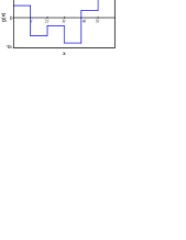
Figure 1: Sample path of the piecewise constant random force $g(x)$ that corresponds to a given realization of the piecewise linear random potential (1).

According to the above assumptions, at $f\in(0,g_{0})$ particles cannot be transported to an arbitrary large distance in the positive direction of the axis $x$. On the contrary, they are stopped at some distance $L=lN$ from the origin, where $N$ is the number of that interval which is characterized by the conditions $f>-g^{(n)}$ (for all $n<N$) and $f\leq-g^{(N)}$. This number depends on the sample paths of $g(x)$ and its mean $\langle N\rangle$ (the angular brackets denote an average over these sample paths) can be easily calculated by introducing the probability $I=\int_{-g_{0}}^{f}dg\,u(g)$ that $g(x)<f$. Indeed, since the random forces $g^{(m)}$ are statistically independent on different intervals, the probability $W_{n}$ that $N=n$ can be written as $W_{n}=I^{n}\int_{f}^{g_{0}}dg\,u(g)$, i.e., $W_{n}=I^{n}-I^{n+1}$. With this expression for $W_{n}$ we obtain $\langle N\rangle=\sum_{n=1}^{\infty}nW_{n}=\sum_{n=1}^{\infty}I^{n}$, and the use of the geometric series formula $\sum_{n=0}^{\infty}I^{n}=1/(1-I)$ yields $\langle N\rangle=I/(1-I)$. As a consequence, the average distance $\langle L\rangle$ to the point where particles are stopped is given by

$$\langle L\rangle=l\,\frac{I}{1-I}.$$ (3)

Thus, if $f<g_{0}$, i.e., $I<1$, then the final state of particles is their localization at a finite average distance (3). We note also that if the probability density $u(g)$ has no $\delta$ singularities at $g=\pm g_{0}$, i.e., $u(g)$ does not contain the terms proportional to $\delta(g-g_{0})$ and $\delta(g+g_{0})$, where $\delta(\cdot)$ is the Dirac $\delta$ function, then $I\to 1$ and $\langle L\rangle\to\infty$ as $f\to g_{0}$.

In contrast, if $f>g_{0}$ then $f+g(X_{t})>0$ and, according to the motion equation (2), $X_{t}\to\infty$ as $t\to\infty$. As it follows from (3), the same behavior holds for $f=g_{0}$ as well. In other words, at $f\geq g_{0}$ particles can be transported to an arbitrary large distance along the positive direction of the $x$-axis. In this cases the distribution of particles on the positive semi-axis $x$ is described by the probability density

$$P(x,t)=\langle\delta(x-X_{t})\rangle$$ (4)

that $X_{t}=x$. Assuming that $X_{t}=nl+X_{t}^{(n)}$ and $X_{t}^{(n)}\in[0,l)$, it is convenient to rewrite the probability density of the particle position in the form

$$P(x,t)=\sum_{n=0}^{\infty}P_{n}(x,t)$$ (5)

with $P_{n}(x,t)=\langle\delta(x-nl-X_{t}^{(n)})\rangle$. In order to calculate $P_{n}(x,t)$, let us first introduce the residence time $\tau^{(n)}$ of a particle in the $n$th interval $[nl,nl+l)$, i.e., time that a particle spends moving from the point $nl$ to the point $nl+l$. Since in the overdamped regime the motion occurs with a constant velocity $v^{(n)}=l/\tau^{(n)}$, we obtain $X_{t}^{(n)}=l(t-\sum_{m=0}^{n-1}\tau^{(m)})/\tau^{(n)}$ if $t-\sum_{m=0}^{n-1}\tau^{(m)}\in[0,\tau^{(n)})$ and

$$P_{n}(x,t)=\left\langle\delta\!\left[x-nl-\frac{l}{\tau^{(n)}}\!\left(t-\sum_{m=0}^{n-1}\tau^{(m)}\right)\right]\right\rangle.$$ (6)

According to (2), the residence time is given by $\tau^{(n)}=\nu l/(f+g^{(n)})$. Because of the properties of $g^{(n)}$, these times in different intervals are statistically independent and distributed with the same probability density $p(\tau)$. Taking into account that $\tau\in[\tau_{\rm{min}},\tau_{\rm{max}}]$ with

$$\tau_{\rm{min}}=\frac{\nu l}{f+g_{0}},\qquad\tau_{\rm{max}}=\frac{\nu l}{f-g_{0}},$$ (7)

from the condition $p(\tau)|d\tau|=u(g)|dg|$ we can express the probability density $p(\tau)$ of the residence time through the probability density $u(g)$ of the random force:

$$p(\tau)=\left\{\begin{array}[]{ll}\displaystyle\frac{\nu l}{\tau^{2}}\,u\!\left(\frac{\nu l}{\tau}-f\right),&\tau\in[\tau_{\rm{min}},\tau_{\rm{max}}]\\[10.0pt] 0,&\rm{otherwise}.\end{array}\right.$$ (8)

In turn, the quantities $P_{n}(x,t)$ can be expressed through $p(\tau)$. Specifically, from the definition (6) at $n=0$ we obtain

$$P_{0}(x,t)=\int_{t}^{\infty}d\tau_{0}p(\tau_{0})\delta\!\left(x-\frac{l}{\tau_{0}}\,t\right).$$ (9)

It is also not difficult to see that $P_{n}(x,t)$ at $n\geq 1$ is given by

$$P_{n}(x,t) = \int_{0}^{t}d\tau_{0}p(\tau_{0})\int_{0}^{t-\tau_{0}}d\tau_{1}p(\tau_{1})\ldots\int_{0}^{t-\sum_{m=0}^{n-2}\tau_{m}}$$ (10)

$$\times d\tau_{n-1}p(\tau_{n-1})\int_{t-\sum_{m=0}^{n-1}\tau_{m}}^{\infty}d\tau_{n}p(\tau_{n})$$

$$\times\delta\!\left[x-nl-\!\frac{l}{\tau_{n}}\!\left(t-\sum_{m=0}^{n-1}\!\tau_{m}\right)\!\right].$$

The last two formulas can be written in a more compact form using the notation $v(t)*w(t)$ for the convolution of two functions $v(t)$ and $w(t)$,

$$v(t)*w(t)=\int_{0}^{t}d\tau\,v(\tau)w(t-\tau).$$ (11)

With this definition, we can introduce the $n$-fold convolution of the probability density of the residence time as follows: $p^{*n}(t)=p^{*n-1}(t)*p(t)$. Assuming also that $p^{*0}(t)=\delta(t)$, we obtain $P_{0}(x,t)=p^{*0}(t)*P_{0}(x,t)$, $P_{n}(x,t)=p^{*n}(t)*P_{0}(x-nl,t)$, and so the probability density of the particle position can be represented in the form

$$P(x,t)=\sum_{n=0}^{\infty}p^{*n}(t)*P_{0}(x-nl,t).$$ (12)

We note that there is a possibility of further simplification of $P(x,t)$ by using the Laplace transform method. However, the representation (12) is quite sufficient for our purpose, i.e., finding the moments of $X_{t}$.

3 Moments of the particle position

The $k$th moment of the particle position is defined in the usual way:

$$\langle X^{k}_{t}\rangle=\int_{0}^{\infty}dxx^{k}P(x,t)\qquad(k=1,2,\ldots).$$ (13)

Substituting (12) into (13) and using (9), for the first moment we obtain

$$\langle X_{t}\rangle=l\sum_{n=0}^{\infty}p^{*n}(t)*\int_{t}^{\infty}d\tau(n+t/\tau)p(\tau).$$ (14)

Because of the convolution structure of the summands in (14), it is reasonable to apply the Laplace transform defined as

$$h_{s}=\mathcal{L}\{h(t)\}=\int_{0}^{\infty}dte^{-st}h(t)$$ (15)

($\rm{Re}\,s>0$) to both sides of this formula. Using the convolution theorem for the Laplace transform, $\mathcal{L}\{v(t)*w(t)\}=v_{s}w_{s}$, this yields

$$\langle X_{t}\rangle_{s}=l\sum_{n=0}^{\infty}p^{n}_{s}\,\mathcal{L}\left\{\int_{t}^{\infty}d\tau(n+t/\tau)p(\tau)\right\}.$$ (16)

By changing the order of integration in the Laplace transform of the integral term, we obtain

$$\displaystyle\mathcal{L}\left\{\int_{t}^{\infty}d\tau(n+t/\tau)p(\tau)\right\}=\int_{0}^{\infty}d\tau p(\tau)\quad\;\;$$

$$\displaystyle\times\int_{0}^{\tau}dt(n+t/\tau)e^{-st}=n\,\frac{1-p_{s}}{s}-\frac{p_{s}}{s}+F_{s},$$ (17)

where

$$F_{s}=\frac{1}{s^{2}}\int_{0}^{\infty}d\tau\,\frac{1-e^{-s\tau}}{\tau}\,p(\tau).$$ (18)

Therefore, taking into account that $\sum_{n=0}^{\infty}p^{n}_{s}=1/(1-p_{s})$ and $\sum_{n=1}^{\infty}np^{n}_{s}=p_{s}/(1-p_{s})^{2}$, formula (16) reduces to

$$\langle X_{t}\rangle_{s}=l\,\frac{F_{s}}{1-p_{s}}.$$ (19)

Finally, applying to (19) the inverse Laplace transform defined as

$$h(t)=\mathcal{L}^{-1}\{h_{s}\}=\frac{1}{2\pi i}\int_{c-i\infty}^{c+i\infty}ds\,e^{st}h_{s}$$ (20)

(the real number $c$ is chosen to be larger than the real parts of all singularities of $h_{s}$), we find the first moment in the form

$$\langle X_{t}\rangle=l\,\mathcal{L}^{-1}\!\left\{\frac{F_{s}}{1-p_{s}}\right\}.$$ (21)

The second moment,

$$\langle X_{t}^{2}\rangle=l^{2}\sum_{n=0}^{\infty}p^{*n}(t)*\int_{t}^{\infty}d\tau(n+t/\tau)^{2}p(\tau),$$ (22)

can also be determined by the method of Laplace transform. The similar calculations lead to

$$\langle X_{t}^{2}\rangle_{s}=l^{2}\sum_{n=0}^{\infty}p^{n}_{s}\,\mathcal{L}\left\{\int_{t}^{\infty}d\tau(n+t/\tau)^{2}p(\tau)\right\},$$ (23)

where

$$\mathcal{L}\left\{\int_{t}^{\infty}d\tau(n+t/\tau)^{2}p(\tau)\right\} = n^{2}\frac{1-p_{s}}{s}+2n\frac{sF_{s}-p_{s}}{s}$$ (24)

$$-\frac{p_{s}}{s}+G_{s}$$

with

$$G_{s}=\frac{2}{s^{3}}\int_{0}^{\infty}d\tau\,\frac{1-(1+s\tau)e^{-s\tau}}{\tau^{2}}\,p(\tau).$$ (25)

Carrying out summation over $n$ in equation (23) [for this purpose we use the above expressions for the series and the formula $\sum_{n=1}^{\infty}n^{2}p^{n}_{s}=p_{s}(1+p_{s})/(1-p_{s})^{3}$], we obtain

$$\langle X_{t}^{2}\rangle_{s}=l^{2}\frac{2p_{s}F_{s}+(1-p_{s})G_{s}}{(1-p_{s})^{2}}$$ (26)

and so

$$\langle X_{t}^{2}\rangle=l^{2}\mathcal{L}^{-1}\!\left\{\frac{2p_{s}F_{s}+(1-p_{s})G_{s}}{(1-p_{s})^{2}}\right\}.$$ (27)

As it will be shown below, the representations (21) and (27) of the moments $\langle X_{t}\rangle$ and $\langle X^{2}_{t}\rangle$ are very useful for finding the short- and long-time behavior of the mean-square displacement of a particle, or the variance of the particle position, defined as

$$\sigma^{2}_{X}(t)=\langle X^{2}_{t}\rangle-\langle X_{t}\rangle^{2}.$$ (28)

In conclusion of this section, we briefly discuss the differences between our model and the continuous-time random walk (CTRW) models. Introduced many years ago MW , the CTRW approach has become one of the most important tools for the study of anomalous transport (see e.g. BG , Hug ; AH ; MK ; Z ; KRS ). In the simplest version of the CTRW is assumed that the random waiting time, i.e., time that a walking particle waits before it jumps to another position, and the random jump size are statistically independent. Since equation (2) describes the continuous motion of a particle, this so-called jump model is in general inapplicable to our case. Due to physical reasons, much attention has also been paid to the case in which the waiting time (considered as the motion time) and the jump size (considered as the passed distance) are coupled in such a way that a walking particle moves with a constant velocity SWK ; MLW ; ZK ; Bar ; SM . However, because of the last condition, this velocity model also does not provide an adequate description of the biased diffusion in a piecewise linear random potential. From this point of view, the CTRW model ZSS in which a walking particle moves with a random velocity could be the most appropriate. But in ZSS is assumed that the random velocity and motion time are statistically independent, while in our case the particle velocity $v^{(n)}=(f+g^{(n)})/\nu$ and the residence time $\tau^{(n)}=\nu l/(f+g^{(n)})$ are perfectly dependent, i.e., $v^{(n)}\tau^{(n)}=l$.

Thus, none of the CTRW models completely describes the considered type of biased diffusion. Nevertheless, if the waiting time is associated with the residence time and the jump size with $l$ then the long-time behavior of $X_{t}$ can be adequately described by the CTRW jump model DK . It is therefore reasonable to compare the behavior of $X_{t}$ with that following from the unidirectional CTRW on a semi-infinite chain of period $l$. Within this approach, the particle position is described by a discrete variable $Y_{t}=lN(t)$, where $N(t)$ is the random number of jumps up to time $t$, and the waiting time is characterized by the same probability density $p(\tau)$. Using the moments of $N(t)$ that are known from the theory of CTRWs (see e.g. Hug ), the first two moments of $Y_{t}$ can be written as

$$\langle Y_{t}\rangle=l\mathcal{L}^{-1}\!\left\{\frac{p_{s}}{s(1-p_{s})}\right\},\;\;\langle Y^{2}_{t}\rangle=l^{2}\mathcal{L}^{-1}\!\left\{\frac{p_{s}^{2}+p_{s}}{s(1-p_{s})^{2}}\right\}\!.$$ (29)

The difference in the time dependence of the variances $\sigma^{2}_{X}(t)$ and $\sigma^{2}_{Y}(t)=\langle Y^{2}_{t}\rangle-\langle Y_{t}\rangle^{2}$ will be clarified in the next sections.

4 Short-time behavior of the variance

The calculation of the inverse Laplace transforms in formulas (21) and (27) is a difficult technical problem. Fortunately, in the short- and long-time limits this problem can be avoided. Such a possibility provides the celebrated Tauberian theorem for the Laplace transform Hug ; Fel which states that if $h(t)$ is a monotonic function and

$$h_{s}=\mathcal{L}\{h(t)\}\sim L\!\left(\frac{1}{s}\right)\!\frac{1}{s^{\rho}}$$ (30)

as $s\to 0$ ($s\to\infty$) then

$$h(t)=\mathcal{L}^{-1}\{h_{s}\}\sim\frac{1}{\Gamma(\rho)}\,L(t)\,t^{\rho-1}$$ (31)

as $t\to\infty$ ($t\to 0$). Here, $\rho\in(0,\infty)$, $\Gamma(x)$ is the gamma function, and $L(t)$ is a slowly varying function at infinity (zero), i.e., $L(\lambda t)\sim L(t)$ as $t\to\infty$ ($t\to 0$) for all $\lambda>0$. It should be stressed that, in contrast to the Laplace transform (15), the parameter $s$ in (30) is assumed to be a positive real number. We note also that if $s\to 0$ then the Tauberian theorem is valid in a more general case, namely, if $h(t)$ is ultimately monotone, i.e., monotone on the interval $(t^{\prime},\infty)$ for some $t^{\prime}>0$.

Thus, for finding the short-time behavior of the moments $\langle X_{t}\rangle$ and $\langle X_{t}^{2}\rangle$ at $f\geq g_{0}$ we should determine the leading terms of the Laplace transforms $\langle X_{t}\rangle_{s}$ and $\langle X_{t}^{2}\rangle_{s}$ as $s$ tends to infinity. Taking into account that $\tau\in[\tau_{\rm{min}},\tau_{\rm{max}}]$ and $p_{s}\to 0$ as $s\to\infty$, from (19) and (26) in this limit we obtain

$$\langle X_{t}\rangle_{s}\sim\frac{l}{s^{2}}\int_{\tau_{\rm{min}}}^{\tau_{\rm{max}}}d\tau\,\frac{p(\tau)}{\tau},\quad\langle X_{t}^{2}\rangle_{s}\sim\frac{2l^{2}}{s^{3}}\int_{\tau_{\rm{min}}}^{\tau_{\rm{max}}}d\tau\,\frac{p(\tau)}{\tau^{2}}.$$ (32)

Using (8) and the symmetry property of the probability density of the random force, $u(-g)=u(g)$, the integrals in (32) can be expressed as

$$\int_{\tau_{\rm{min}}}^{\tau_{\rm{max}}}d\tau\,\frac{p(\tau)}{\tau}=\frac{f}{\nu l},\quad\int_{\tau_{\rm{min}}}^{\tau_{\rm{max}}}d\tau\,\frac{p(\tau)}{\tau^{2}}=\frac{f^{2}+\sigma^{2}_{g}}{(\nu l)^{2}},$$ (33)

where $\sigma^{2}_{g}=\int_{-g_{0}}^{g_{0}}dgg^{2}u(g)$ is the variance of the random force $g(x)$. Therefore, as follows from the Tauberian theorem, the short-time behavior of the first two moments is described by the asymptotic formulas

$$\langle X_{t}\rangle\sim\frac{f}{\nu}\,t,\quad\langle X_{t}^{2}\rangle\sim\frac{f^{2}+\sigma^{2}_{g}}{\nu^{2}}\,t^{2}.$$ (34)

They show that at small times ($t\ll\nu l/f$) and $f\geq g_{0}$ the biased diffusion is always ballistic, i.e., $\sigma^{2}_{X}(t)$ is proportional to $t^{2}$:

$$\sigma^{2}_{X}(t)\sim\frac{\sigma^{2}_{g}}{\nu^{2}}\,t^{2}.$$ (35)

We note that the diffusion law (35) also follows from the motion equation (2). Indeed, the first two moments of the particle position $X_{t}\sim t(f+g^{(0)})/\nu$, which is the solution of this equation at $t\to 0$, are the same as in (34).

For finding the short-time behavior of the moments of the discrete variable $Y_{t}$ the Tauberian theorem cannot be used. The reason is that $\langle Y_{t}^{k}\rangle_{s}$ at $s\to\infty$ tends to zero more rapidly than any positive power of $1/s$ (since $p_{s}\propto e^{-s\tau_{\rm{min}}}$ as $s\to\infty$). Nevertheless, exact conclusions about the short-time behavior of $\langle Y_{t}^{k}\rangle$ can be drown directly from the definition $\langle Y_{t}^{k}\rangle=l^{k}\sum_{n=1}^{\infty}n^{k}\mathcal{P}(n,t)$, where $\mathcal{P}(n,t)$ is the probability that $N(t)=n$. Indeed, accounting for the fact that $\mathcal{P}(n,t)=p(t)*\mathcal{P}(n-1,t)$ ($n\geq 1$) and $\mathcal{P}(0,t)=\int_{t}^{\infty}d\tau p(\tau)$ Hug , we make sure (see also (8) and (11)) that if $t<\tau_{\rm{min}}$ then $\mathcal{P}(0,t)=1$ and $\mathcal{P}(n,t)=0$ for all $n\geq 1$. Hence, at $t<\tau_{\rm{min}}$ all moments of $Y_{t}$ are equal to zero and so the short-time behavior of $Y_{t}$ is qualitatively different from that for $X_{t}$.

5 Long-time behavior of the variance

5.1 Conditions of normal and anomalous diffusion

According to (8), the $m$th moment of the residence time, $\overline{\tau^{m}}=\int_{0}^{\infty}d\tau\tau^{m}p(\tau)$ $(m=1,2,\ldots)$, can be written in the form

$$\overline{\tau^{m}}=(\nu l)^{m}\int_{-g_{0}}^{g_{0}}dg\,\frac{u(g)}{(f+g)^{m}}.$$ (36)

Since the probability density $u(g)$ is properly normalized on the interval $[-g_{0},g_{0}]$, i.e., $\int_{-g_{0}}^{g_{0}}dgu(g)=1$, the above formula leads to the condition $\overline{\tau^{m}}\leq(\nu l)^{m}/(f-g_{0})^{m}$. It shows that if $f>g_{0}$ then all moments $\overline{\tau^{m}}$ are finite. Since in this case $\overline{\tau^{2}}<\infty$, the classical central limit theorem for sums of a random number of random variables GK is applied to $X_{t}$ and suggests that $\sigma^{2}_{X}(t)\propto t$ as $t\to\infty$. In other words, at $f>g_{0}$ the biased diffusion of particles is expected to be always normal.

In contrast, if $f=g_{0}$ then the residence time varies from $\tau_{\rm{min}}=\nu l/2g_{0}$ to $\tau_{\rm{max}}=\infty$, and $\overline{\tau^{2}}$ can be either finite or infinite depending on the asymptotic behavior of $p(\tau)$ as $\tau\to\infty$ (i.e., asymptotic behavior of $u(g)$ as $g\to-g_{0}$). While in the former case the biased diffusion is also expected to be normal, in the latter (when $\overline{\tau^{2}}=\infty$) the above mentioned central limit theorem becomes inapplicable and one may expect that the biased diffusion is anomalous. Next we assume that at $f=g_{0}$ the probability density $p(\tau)$ of the residence time is characterized by the asymptotic formula

$$p(\tau)\sim\frac{a}{\tau^{1+\alpha}}\quad(\tau\to\infty)$$ (37)

with positive parameters $a$ and $\alpha$. According to it $\overline{\tau^{2}}<\infty$ if $\alpha>2$ and $\overline{\tau^{2}}=\infty$ if $\alpha\in(0,2]$. The parameters $a$ and $\alpha$ depend on the explicit form of the probability density $u(g)$ of the piecewise constant random force $g(x)$ and are in general not independent. In particular, for the symmetric beta probability density

$$u(g)=\frac{\Gamma(\beta+1/2)}{g_{0}\sqrt{\pi}\,\Gamma(\beta)}\!\left(1-\frac{g^{2}}{g_{0}^{2}}\right)^{\!\beta-1}$$ (38)

($\beta>0$) we have $\alpha=\beta$ and

$$a=\!\left(\frac{2\nu l}{g_{0}}\right)^{\!\alpha}\frac{\Gamma(\alpha+1/2)}{2\sqrt{\pi}\,\Gamma(\alpha)}.$$ (39)

Thus, the biased diffusion is expected to be normal if $f>g_{0}$ or $f=g_{0}$ and $\alpha>2$, and anomalous if $f=g_{0}$ and $\alpha\in(0,2]$. In the next two sections we validate these criteria and derive the laws of normal and anomalous diffusion.

5.2 Normal biased diffusion

5.2.1 Modified Tauberian theorem.

The ordinary Tauberian theorem formulated in (30) and (31) permits us to find only the leading terms of the asymptotic expansion of $h(t)$ at $t\to 0$ and $t\to\infty$. Therefore, in this form it can be used for determining the long-time behavior of the variance $\sigma^{2}_{X}(t)$ only in the case when the leading terms of $\langle X_{t}\rangle^{2}$ and $\langle X^{2}_{t}\rangle$ are different (see section 5.3.1). But in order to find $\sigma^{2}_{X}(t)$ in the case with $\langle X_{t}\rangle^{2}\sim\langle X^{2}_{t}\rangle$, we need to know at least two leading terms of each of the asymptotic expansions of $\langle X_{t}\rangle$ and $\langle X^{2}_{t}\rangle$. With one exception (see section 5.3.3), these terms can be found by applying the modified version of the Tauberian theorem. This version follows directly from the ordinary one by replacing $h_{s}$ by $h_{s}-r/s^{\eta}$ and using the exact result $\mathcal{L}^{-1}\{1/s^{\eta}\}=t^{\eta-1}/\Gamma(\eta)$ Erd . According to this, we formulate the modified Tauberian theorem as follows: If $h(t)-rt^{\eta-1}/\Gamma(\eta)$ is ultimately monotone and

$$h_{s}\sim\frac{r}{s^{\eta}}+L\!\left(\frac{1}{s}\right)\!\frac{1}{s^{\rho}}$$ (40)

($\eta>\rho>0$) as $s\to 0$ then

$$h(t)\sim\frac{r}{\Gamma(\eta)}\,t^{\eta-1}+\frac{1}{\Gamma(\rho)}\,L(t)\,t^{\rho-1}$$ (41)

as $t\to\infty$.

It is important to emphasize that the terms $rt^{\eta-1}/\Gamma(\eta)$ and $L(t)t^{\rho-1}/\Gamma(\rho)$ represent the first two terms of the long-time expansion of $h(t)$ only if $\eta>\rho$. The reason is that in the opposite case (when $\eta\leq\rho$) the second term of the asymptotic expansion of $\mathcal{L}^{-1}\{L(1/s)/s^{\rho}\}$ at $t\to\infty$ may not be negligible in comparison with $\mathcal{L}^{-1}\{r/s^{\eta}\}$. In order to illustrate this fact, we assume that $L(1/s)=\ln(1/s)$ and consider the Laplace transform of the following form:

$$h_{s}=\frac{1}{s^{\eta}}+\ln\!\left(\frac{1}{s}\right)\!\frac{1}{s^{\rho}}.$$ (42)

Since $\mathcal{L}^{-1}\!\{\ln(1/s)/s^{\rho}\}=t^{\rho-1}[\ln t-\psi(\rho)]/\Gamma(\rho)$ Erd , where $\psi(\rho)$ is the digamma function, i.e., the logarithmic derivative of the gamma function $\Gamma(\rho)$, the inverse Laplace transform of $h_{s}$ yields an exact result

$$h(t)=\frac{t^{\eta-1}}{\Gamma(\eta)}+\frac{t^{\rho-1}}{\Gamma(\rho)}\,[\ln t-\psi(\rho)].$$ (43)

Keeping in the long-time limit two leading terms of $h(t)$, we obtain

$$h(t)\sim\left\{\begin{array}[]{ll}t^{\eta-1}/\Gamma(\eta)+t^{\rho-1}\ln t/\Gamma(\rho),&\eta>\rho\\[6.0pt] t^{\eta-1}[\ln t-\psi(\eta)+1]/\Gamma(\eta),&\eta=\rho\\[6.0pt] t^{\rho-1}[\ln t-\psi(\rho)]/\Gamma(\rho),&\eta<\rho.\end{array}\right.$$ (44)

By comparing the asymptotic formulas (41) and (44) we make sure that at $\eta>\rho$ and $t\to\infty$ two leading terms of $h(t)$ can indeed be determined from the modified Tauberian theorem. In contrast, if $\eta\leq\rho$ then for finding two leading terms of the long-time expansion of $h(t)$ it is necessary to go beyond the Tauberian theorem.

5.2.2 Properties of the diffusion coefficient.

We define the coefficient of biased diffusion in the same way as for ordinary diffusion:

$$D_{\rm{b}}=\lim_{t\to\infty}\frac{\sigma^{2}_{X}(t)}{2t}.$$ (45)

As it follows from the modified Tauberian theorem and the definition (28), for determining the law of biased diffusion, i.e., the long-time behavior of the variance $\sigma^{2}_{X}(t)$, we should find two leading terms of each Laplace transform, $\langle X_{t}\rangle_{s}$ and $\langle X_{t}^{2}\rangle_{s}$, in the limit $s\to 0$. Assuming that the first two moments of the residence time, $\overline{\tau}$ and $\overline{\tau^{2}}$, exist, the Laplace transforms $p_{s}$ and $F_{s}$ at $s\to 0$ can be represented by the following asymptotic formulas: $p_{s}\sim 1-s\overline{\tau}+s^{2}\overline{\tau^{2}}/2$ and $F_{s}\sim 1/s-\overline{\tau}/2$. Substituting them into (19), we obtain the desired result

$$\langle X_{t}\rangle_{s}\sim\frac{l}{\overline{\tau}}\frac{1}{s^{2}}+l\frac{\overline{\tau^{2}}-\overline{\tau}^{2}}{2\overline{\tau}^{2}}\frac{1}{s}.$$ (46)

Similarly, taking also into account that $G_{s}\sim 1/s$ as $s\to 0$, from (26) we find with the required accuracy

$$\langle X_{t}^{2}\rangle_{s}\sim\frac{2l^{2}}{\overline{\tau}^{2}}\frac{1}{s^{3}}+2l^{2}\frac{\overline{\tau^{2}}-\overline{\tau}^{2}}{\overline{\tau}^{3}}\frac{1}{s^{2}}.$$ (47)

The asymptotic formulas (46) and (47) are particular cases of (40) in which $L(1/s)$ is a constant. Therefore, the modified Tauberian theorem leads to the following expressions for the moments $\langle X_{t}\rangle$ and $\langle X_{t}^{2}\rangle$ in the long-time limit:

$$\langle X_{t}\rangle\sim\frac{l}{\overline{\tau}}\,t+l\frac{\overline{\tau^{2}}-\overline{\tau}^{2}}{2\overline{\tau}^{2}},\quad\langle X_{t}^{2}\rangle\sim\frac{l^{2}}{\overline{\tau}^{2}}\,t^{2}+2l^{2}\frac{\overline{\tau^{2}}-\overline{\tau}^{2}}{\overline{\tau}^{3}}\,t,$$ (48)

which in turn determine the law of biased diffusion

$$\sigma^{2}_{X}(t)\sim l^{2}\frac{\overline{\tau^{2}}-\overline{\tau}^{2}}{\overline{\tau}^{3}}\,t.$$ (49)

Thus, it follows from (45) and (49) that the coefficient of biased diffusion can be written as

$$D_{\rm{b}}=l^{2}\frac{\overline{\tau^{2}}-\overline{\tau}^{2}}{2\overline{\tau}^{3}}.$$ (50)

Using (36) and the Jensen inequality Fel , one can see that for all probability densities $u(g)$ the condition $D_{\rm{b}}\in[0,\infty]$ holds. However, if $f>g_{0}$ then the moments $\overline{\tau}$ and $\overline{\tau^{2}}$ are finite (see section 5.1) and nonzero (see formula (36)), i.e., $D_{\rm{b}}\neq\infty$. On the other hand, representing $\overline{\tau^{2}}$ as

$$\overline{\tau^{2}} = \frac{(\nu l)^{2}}{2}\int_{-g_{0}}^{g_{0}}\int_{-g_{0}}^{g_{0}}dgdg^{\prime}u(g)u(g^{\prime})$$ (51)

$$\times\left(\frac{1}{(f+g)^{2}}+\frac{1}{(f+g^{\prime})^{2}}\right)$$

and $\overline{\tau}^{2}$ as

$$\overline{\tau}^{2}=(\nu l)^{2}\int_{-g_{0}}^{g_{0}}\int_{-g_{0}}^{g_{0}}dgdg^{\prime}\frac{u(g)u(g^{\prime})}{(f+g)(f+g^{\prime})},$$ (52)

we obtain

$$\overline{\tau^{2}}-\overline{\tau}^{2} = \frac{(\nu l)^{2}}{2}\int_{-g_{0}}^{g_{0}}\int_{-g_{0}}^{g_{0}}dgdg^{\prime}u(g)u(g^{\prime})$$ (53)

$$\times\frac{(g-g^{\prime})^{2}}{(f+g)^{2}(f+g^{\prime})^{2}}.$$

The last expression shows that always $\overline{\tau^{2}}-\overline{\tau}^{2}\geq 0$, and the condition $\overline{\tau^{2}}=\overline{\tau}^{2}$ ($D_{\rm{b}}=0$) holds only if $u(g)=\delta(g)$ (we took into account the condition $u(-g)=u(g)$). But the probability density $u(g)=\delta(g)$ corresponds to the trivial case when the random force $g(x)$ is absent. Excluding it from consideration, we obtain $D_{\rm{b}}\neq 0$. Thus, if $f>g_{0}$ then $D_{\rm{b}}\in(0,\infty)$, i.e., the biased diffusion is normal: $\sigma^{2}_{X}(t)\sim 2D_{\rm{b}}t$. It is clear from the above analysis that at $f=g_{0}$ and $\alpha>2$ the biased diffusion is also normal. In contrast, if $D_{\rm{b}}=0$ or $D_{\rm{b}}=\infty$ (these conditions are realized only if $f=g_{0}$ and $\alpha\in(0,2]$, see section 5.3) then the biased diffusion becomes anomalous: It is slower than normal in the former case and is faster in the latter one. We note, however, that the conditions $D_{\rm{b}}=0$ and $D_{\rm{b}}=\infty$ only indicate the existence of anomalous behavior and cannot be used for finding the laws of anomalous diffusion.

Next we consider the dependence of $D_{\rm{b}}$ on the external force $f$ and statistical characteristics of the random force $g(x)$. Let us first determine $D_{\rm{b}}$ in the case of large external force when $f\gg g_{0}$. By expanding the integrand of (36) in powers of $g/f$ and integrating over $g$ with the condition $u(-g)=u(g)$, we obtain

$$\overline{\tau}\sim\frac{\nu l}{f}\!\left(1+\frac{\sigma^{2}_{g}}{f^{2}}\right)\!,\quad\overline{\tau^{2}}\sim\left(\frac{\nu l}{f}\right)^{2}\!\left(1+3\frac{\sigma^{2}_{g}}{f^{2}}\right)$$ (54)

as $f\to\infty$. The substitution of these asymptotic expressions into (50) leads to the universal, inversely proportional dependence of $D_{\rm{b}}$ on $f$ for large values of $f$:

$$D_{\rm{b}}\sim\frac{l\sigma^{2}_{g}}{2\nu}\,\frac{1}{f}.$$ (55)

If $f>g_{0}$ and the probability density $u(g)$ is given by (38) then, according to (36), the moments of the residence time can be represented in the form

$$\overline{\tau^{m}}=\left(\frac{\nu l}{f-g_{0}}\right)^{m}\!F\!\left(m,\beta;2\beta;-\frac{2g_{0}}{f-g_{0}}\right),$$ (56)

where $F(m,\beta;2\beta;z)=\!\,_{2}F_{1}(m,\beta;2\beta;z)$ is the hypergeometric function. In some cases the first two moments, $\overline{\tau}$ and $\overline{\tau^{2}}$, can be expressed in elementary functions. In particular, it is possible for $\beta=1$, i.e., if $u(g)$ corresponds to a uniform distribution of the random force $g(x)$ on the interval $[-g_{0},g_{0}]$. In this case, using the conditions AS $F(1,1;2;z)=-z^{-1}\ln(1-z)$, $F(m,\beta;2\beta;z)=F(\beta,m;2\beta;z)$ and $F(1,2;2;z)=(1-z)^{-1}$, we get

$$\overline{\tau}=\frac{\nu l}{2g_{0}}\,\ln\frac{q+1}{q-1},\quad\overline{\tau^{2}}=\left(\frac{\nu l}{g_{0}}\right)^{2}\frac{1}{q^{2}-1}$$ (57)

and, as a consequence,

$$D_{\rm{b}}=\frac{lg_{0}}{\nu}\!\left(\frac{4}{q^{2}-1}-\ln^{2}\frac{q+1}{q-1}\right)\ln^{-3}\frac{q+1}{q-1},$$ (58)

where $q=f/g_{0}>1$ is the dimensionless external force. The coefficient of biased diffusion (58) is a monotonically decreasing function of $q$ (see figure 2) which tends to infinity as $q\to 1$, $D_{\rm{b}}\sim(2lg_{0}/\nu)(q-1)^{-1}|\ln^{-3}(q-1)|$, and approaches zero as $q\to\infty$, $D_{\rm{b}}\sim(lg_{0}/6\nu)q^{-1}$. Since for the uniform distribution $\sigma^{2}_{g}=g_{0}^{2}/3$, the last asymptotic formula coincides with that given in (55).

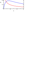
Figure 2: The reduced coefficient of unidirectional diffusion $D=D_{\rm{b}}\nu/lg_{0}$ as a function of the dimensionless driving force $q=f/g_{0}$. The monotonic dependence of $D$ on $q$ is determined from formula (58) which corresponds to the uniform probability density $u(g)$, and the non-monotonic one follows from formula (63) which corresponds to the probability density (61).

Formula (56) is also valid in the limit $f\to g_{0}$. However, in order to find explicit expressions for $\overline{\tau}$ and $\overline{\tau^{2}}$, it is much more convenient to use the basic formula (36) with $f=g_{0}$. A straightforward integration in this case yields

$$\overline{\tau}=\frac{\nu l}{g_{0}}\,\frac{2\beta-1}{2(\beta-1)},\quad\overline{\tau^{2}}=\left(\frac{\nu l}{g_{0}}\right)^{2}\frac{2\beta-1}{2(\beta-2)}$$ (59)

for $\beta>1$ and $\beta>2$, respectively. Therefore, if $f=g_{0}$ (i.e., $q=1$) and $\beta>2$ then

$$D_{\rm{b}}=\frac{lg_{0}}{\nu}\,\frac{\beta(\beta-1)}{(2\beta-1)^{2}(\beta-2)}.$$ (60)

A quite different behavior of $D_{\rm{b}}$ on $q$ occurs if the probability density $u(g)$ is mainly concentrated near the edges of the interval $[-g_{0},g_{0}]$. In particular, for the limiting case characterized by the probability density

$$u(g)=\frac{1}{2}\,\delta(g-g_{0})+\frac{1}{2}\,\delta(g+g_{0})$$ (61)

we obtain

$$\overline{\tau}=\frac{\nu l}{g_{0}}\,\frac{q}{q^{2}-1},\quad\overline{\tau^{2}}=\left(\frac{\nu l}{g_{0}}\right)^{2}\frac{q^{2}+1}{(q^{2}-1)^{2}}$$ (62)

and so

$$D_{\rm{b}}=\frac{lg_{0}}{2\nu}\,\frac{q^{2}-1}{q^{3}}.$$ (63)

In contrast to the previous case, now $D_{\rm{b}}$ is a non-monotonic function of $q$ (see figure 2). According to (63), $D_{\rm{b}}\sim(lg_{0}/2\nu)q^{-1}$ as $q\to\infty$ (since in this case $\sigma^{2}_{g}=g^{2}_{0}$, the same result follows from (55) as well), $D_{\rm{b}}\sim(lg_{0}/\nu)(q-1)$ as $q\to 1$, and the maximum value of $D_{\rm{b}}$ is $D_{\rm{b}}\big{|}_{q=\sqrt{3}}\approx 0.192\!\times\!(lg_{0}/\nu)$.

5.3 Anomalous biased diffusion

According to the above analysis, the biased diffusion is anomalous if both conditions $f=g_{0}$ and $\alpha\in(0,2]$ hold. Specifically, if $\alpha\in(1,2]$ then $\overline{\tau^{2}}=\infty$, $\overline{\tau}<\infty$ and so $D_{\rm{b}}=\infty$, i.e., the biased diffusion is fast in comparison with normal. In contrast, if $\alpha\in(0,1]$ then $\overline{\tau^{2}}=\infty$, $\overline{\tau}=\infty$, and depending on $\alpha$ the biased diffusion can be fast ($D_{\rm{b}}=\infty$), slow ($D_{\rm{b}}=0$) or even formally normal ($0<D_{\rm{b}}<\infty$). Thus, taking into account that the points $\alpha=1$ and $\alpha=2$ are distinct, we consider the long-time behavior of the variance $\sigma^{2}_{X}(t)$ separately for $\alpha\in(0,1)$, $\alpha\in(1,2)$, $\alpha=1$, and $\alpha=2$.

5.3.1 $\alpha\in(0,1)$.

Since in this case the leading terms of $\langle X_{t}\rangle^{2}$ and $\langle X_{t}^{2}\rangle$ are different (see below), for their finding we need to know only two leading terms of $p_{s}$ as $s\to 0$. These two terms can be easily evaluated using the expression

$$p_{s}=1-\frac{1}{s}\int_{s\tau_{\rm{min}}}^{\infty}dy(1-e^{-y})p\!\left(\frac{y}{s}\right),$$ (64)

which follows from the definition $p_{s}=\int_{\tau_{\rm{min}}}^{\infty}d\tau e^{-s\tau}p(\tau)$ and the normalization condition $\int_{\tau_{\rm{min}}}^{\infty}d\tau p(\tau)=1$ (we recall that $\tau_{\rm{min}}=\nu l/2g_{0}$ and $\tau_{\rm{max}}=\infty$ at $f=g_{0}$). Keeping in (64) the leading term of the asymptotic expansion of the integral as $s\to 0$ and using asymptotic formula (37) and the integral representation of the gamma function AS , $\Gamma(x)=\int_{0}^{\infty}dy\,e^{-y}y^{x-1}$, we obtain the desired result

$$p_{s}\sim 1-\frac{a\Gamma(1-\alpha)}{\alpha}\,s^{\alpha}.$$ (65)

In order to find the leading terms of $F_{s}$ and $G_{s}$, it is convenient to introduce the new variable of integration $y=s\tau$ and rewrite expressions (18) and (25) in the form

$$F_{s}=\frac{1}{s}-\frac{1}{s^{2}}\int_{s\tau_{\rm{min}}}^{\infty}dy\,\frac{e^{-y}+y-1}{y}\,p\!\left(\frac{y}{s}\right)$$ (66)

and

$$G_{s}=\frac{1}{s}-\frac{2}{s^{2}}\int_{s\tau_{\rm{min}}}^{\infty}dy\,\frac{(1+y)e^{-y}+y^{2}/2-1}{y^{2}}\,p\!\left(\frac{y}{s}\right).$$ (67)

Using the asymptotic formula (37), one can make sure that the integral terms in (66) and (67) are proportional to $1/s^{1-\alpha}$ and so $F_{s}\sim G_{s}\sim 1/s$ as $s\to 0$. Thus, in accordance with this result and asymptotic expression (65) the leading terms of the Laplace transforms (19) and (26) take the form

$$\langle X_{t}\rangle_{s}\sim\frac{l\alpha}{a\Gamma(1-\alpha)}\frac{1}{s^{1+\alpha}},\quad\langle X_{t}^{2}\rangle_{s}\sim\frac{2l^{2}\alpha^{2}}{a^{2}\Gamma^{2}(1-\alpha)}\frac{1}{s^{1+2\alpha}}.$$ (68)

These asymptotic formulas are particular cases of the asymptotic formula (30) in which the slowly varying function $L(1/s)$ is a constant. Therefore, as follows from (31), the long-time dependence of the moments $\langle X_{t}\rangle$ and $\langle X_{t}^{2}\rangle$ is given by

$$\langle X_{t}\rangle\sim\frac{l\alpha}{a\Gamma(1-\alpha)\Gamma(1+\alpha)}\,t^{\alpha}$$ (69)

and

$$\langle X_{t}^{2}\rangle\sim\frac{2l^{2}\alpha^{2}}{a^{2}\Gamma^{2}(1-\alpha)\Gamma(1+2\alpha)}\,t^{2\alpha}.$$ (70)

As it seen from these asymptotic formulas, the leading terms of $\langle X_{t}\rangle^{2}$ and $\langle X_{t}^{2}\rangle$ are different and so

$$\sigma^{2}_{X}(t)\sim\frac{l^{2}\alpha^{2}}{a^{2}\Gamma^{2}(1-\alpha)}\left(\!\frac{2}{\Gamma(1+2\alpha)}-\frac{1}{\Gamma^{2}(1+\alpha)}\right)\!t^{2\alpha}.$$ (71)

According to (71), the biased diffusion is characterized by a subdiffusive behavior (with $D_{\rm{b}}=0$) if $\alpha\in(0,1/2)$ and by a superdiffusive one (with $D_{\rm{b}}=\infty$) if $\alpha\in(1/2,1)$. At $\alpha=1/2$ the diffusion is formally normal with $D_{\rm{b}}=l^{2}(\pi-2)/(2\pi a)^{2}$. However, since $\overline{\tau}=\infty$, $\overline{\tau^{2}}=\infty$ and $\langle X_{t}\rangle\propto t^{1/2}$, we term this type of biased diffusion the quasi-normal diffusion. We note also that the asymptotic formula (71) agrees with the asymptotic solution of the CTRWs Shles .

5.3.2 $\alpha\in(1,2)$.

In this and all other cases the leading terms of $\langle X_{t}\rangle^{2}$ and $\langle X_{t}^{2}\rangle$ are the same. Therefore, for finding $\sigma^{2}_{X}(t)$ we need to determine three leading terms of $p_{s}$ as $s\to 0$. Since for these values of $\alpha$ the mean residence time $\overline{\tau}=\int_{\tau_{\rm{min}}}^{\infty}d\tau\tau p(\tau)$ exists, to this end it is convenient to use the following exact formula:

$$p_{s}=1-\overline{\tau}s+\frac{1}{s}\int_{s\tau_{\rm{min}}}^{\infty}dy(e^{-y}+y-1)p\!\left(\frac{y}{s}\right).$$ (72)

Proceeding in the same way as before, at $s\to 0$ we obtain

$$p_{s}\sim 1-\overline{\tau}s+\frac{a\Gamma(2-\alpha)}{\alpha(\alpha-1)}\,s^{\alpha}.$$ (73)

Then, from (66) and (67) it follows that $F_{s}\sim 1/s-\overline{\tau}/2$ and $G_{s}\sim 1/s-2\overline{\tau}/3$ as $s\to 0$. Taking also into account that in the main approximation $F_{s}\sim 1/s$ and $2p_{s}F_{s}+(1-p_{s})G_{s}\sim 2/s$, the Laplace transforms (19) and (26) are reduced to

$$\langle X_{t}\rangle_{s}\sim\frac{l}{\overline{\tau}}\frac{1}{s^{2}}+\frac{la\Gamma(2-\alpha)}{\overline{\tau}^{2}\alpha(\alpha-1)}\frac{1}{s^{3-\alpha}}$$ (74)

and

$$\langle X_{t}^{2}\rangle_{s}\sim\frac{2l^{2}}{\overline{\tau}^{2}}\frac{1}{s^{3}}+\frac{4l^{2}a\Gamma(2-\alpha)}{\overline{\tau}^{3}\alpha(\alpha-1)}\frac{1}{s^{4-\alpha}}.$$ (75)

Finally, applying the modified Tauberian theorem to (74) and (75) and using the well-known property of the gamma function, $\Gamma(1+x)=x\Gamma(x)$, we get

$$\langle X_{t}\rangle\sim\frac{l}{\overline{\tau}}\,t+\frac{la}{\overline{\tau}^{2}\alpha(\alpha-1)(2-\alpha)}\,t^{2-\alpha}$$ (76)

and

$$\langle X_{t}^{2}\rangle\sim\frac{l^{2}}{\overline{\tau}^{2}}\,t^{2}+\frac{4l^{2}a}{\overline{\tau}^{3}\alpha(\alpha-1)(2-\alpha)(3-\alpha)}\,t^{3-\alpha}.$$ (77)

as $t\to\infty$. As it follows from (76) and (77), the long-time behavior of the variance $\sigma^{2}_{X}(t)$ obeys the asymptotic power law

$$\sigma^{2}_{X}(t)\sim\frac{2l^{2}a}{\overline{\tau}^{3}\alpha(2-\alpha)(3-\alpha)}\,t^{3-\alpha}.$$ (78)

It shows that at $\alpha\in(1,2)$ the unidirectional transport of particles is superdiffusive. The parameters in (78) depend on the probability density $u(g)$ of the random force. In particular, if $u(g)$ is determined by (38) then $\alpha=\beta$, the parameter $a$ is given by (39), and

$$\overline{\tau}=\frac{\nu l}{g_{0}}\,\frac{\alpha-1/2}{\alpha-1}.$$ (79)

5.3.3 $\alpha=1$.

In order to illustrate the distinctive features of the long-time dependence of the moments $\langle X_{t}\rangle$ and $\langle X_{t}^{2}\rangle$ at $\alpha=1$, i.e., when according to (37) $p(\tau)\sim a/\tau^{2}$ ($\tau\to\infty$), we first represent the Laplace transform $p_{s}$ in the form

$$p_{s}=1-aq_{s}-\frac{1}{s}\int_{s\tau_{\rm{min}}}^{\infty}dy(1-e^{-y})\!\left[p\!\left(\frac{y}{s}\right)-a\frac{s^{2}}{y^{2}}\right]\!,$$ (80)

where $q_{s}=s\int_{s\tau_{\rm{min}}}^{\infty}dy(1-e^{-y})/y^{2}$. With the definition of the exponential integral AS , $E_{1}(x)=\int_{x}^{\infty}dy\,e^{-y}/y$, the last quantity can be written as

$$q_{s}=\frac{1-e^{-s\tau_{\rm{min}}}}{\tau_{\rm{min}}}+sE_{1}(s\tau_{\rm{min}}).$$ (81)

Then, since $p(\tau)-a/\tau^{2}=o(1/\tau^{2})$ as $\tau\to\infty$ (we recall that $p(\tau)\sim a/\tau^{2}$ if $f=g_{0}$ and $\alpha=1$), the integral term in (80) at $s\to 0$ can be neglected in comparison with the term $aq_{s}$. Finally, using the asymptotic formula $E_{1}(s\tau_{\rm{min}})\sim\ln(1/s)$ ($s\to 0$) AS , we obtain

$$p_{s}\sim 1-as\ln\frac{1}{s}.$$ (82)

As it can be easily seen, the integral terms in (66) and (67) at $\alpha=1$ are proportional to $\ln(1/s)$ and so $F_{s}\sim G_{s}\sim 1/s$ ($s\to 0$). Therefore, the leading terms of the Laplace transforms (19) and (26) can be written in the form

$$\langle X_{t}\rangle_{s}\sim\frac{l}{a}\frac{1}{s^{2}\ln(1/s)},\quad\langle X_{t}^{2}\rangle_{s}\sim\frac{l^{2}}{a^{2}}\frac{2}{s^{3}\ln^{2}(1/s)}$$ (83)

($s\to 0$) that in accordance with (31) yields

$$\langle X_{t}\rangle\sim\frac{l}{a}\frac{t}{\ln t},\quad\langle X_{t}^{2}\rangle\sim\frac{l^{2}}{a^{2}}\frac{t^{2}}{\ln^{2}t}$$ (84)

($t\to\infty$). Since $\langle X_{t}\rangle^{2}\sim\langle X_{t}^{2}\rangle$, for finding the long-time behavior of the variance $\sigma^{2}_{X}(t)$ we need to know at least two terms of the asymptotic expansion of $\langle X_{t}\rangle$ and $\langle X_{t}^{2}\rangle$. However, in contrast to the previous case they cannot be determined from the modified Tauberian theorem because the leading terms of $\langle X_{t}\rangle_{s}$ and $\langle X_{t}^{2}\rangle_{s}$ contain the slowly varying functions, see (83). As it was mentioned in section 5.2.1, in this case it is necessary to go beyond the Tauberian theorem. Nevertheless, using the asymptotic laws (71) and (78), we can make some qualitative conclusions about the character of biased diffusion at $\alpha=1$. First of all, it follows from (71) and (78) that $t^{2\alpha}$ and $t^{3-\alpha}$ tend to $t^{2}$ as $\alpha\to 1-0$ and $\alpha\to 1+0$, respectively. But since $\Gamma(1-\alpha)\to\infty$ as $\alpha\to 1-0$ and $\overline{\tau}\to\infty$ as $\alpha\to 1+0$, the coefficients of proportionality between $\sigma^{2}_{X}(t)$ and $t^{2}$ tend to zero. This means that at $\alpha=1$ the weakened ballistic diffusion should occur.

5.3.4 $\alpha=2$.

If $\alpha=2$ then it is convenient to represent the Laplace transform $p_{s}$ as

$$p_{s}=1-\overline{\tau}s-ar_{s}-\frac{1}{s}\!\int_{s\tau_{\rm{min}}}^{\infty}\!dy(1-y-e^{-y})\!\left[p\!\left(\frac{y}{s}\right)-a\frac{s^{3}}{y^{3}}\right]\!,$$ (85)

where

$$r_{s} = s^{2}\int_{s\tau_{\rm{min}}}^{\infty}dy\,\frac{1-y-e^{-y}}{y^{3}}$$ (86)

$$= \frac{1-2s\tau_{\rm{min}}\!-(1-s\tau_{\rm{min}})e^{-s\tau_{\rm{min}}}}{2\tau_{\rm{min}}^{2}}-\frac{s^{2}}{2}E_{1}(s\tau_{\rm{min}}).\qquad$$

Taking into account that $p(\tau)-a/\tau^{3}=o(1/\tau^{3})$ ($\tau\to\infty$), the integral term in (85) at $s\to 0$ can be neglected in comparison with $ar_{s}\sim-(as^{2}/2)\ln(1/s)$. Therefore, keeping in $p_{s}$ three leading terms, one obtains

$$p_{s}\sim 1-\overline{\tau}s+\frac{a}{2}s^{2}\ln\frac{1}{s}.$$ (87)

Asymptotic expression (87) shows that for determining two leading terms of $\langle X_{t}\rangle_{s}$ and $\langle X_{t}^{2}\rangle_{s}$ only the leading terms of $F_{s}$ and $G_{s}$ should be kept. Since $F_{s}\sim G_{s}\sim 1/s$, from (19), (26) and (87) we immediately find

$$\langle X_{t}\rangle_{s}\sim\frac{l}{\overline{\tau}}\frac{1}{s^{2}}+\frac{la}{2\overline{\tau}^{2}}\frac{1}{s}\ln\!\frac{1}{s},\quad\displaystyle\langle X_{t}^{2}\rangle_{s}\sim\frac{2l^{2}}{\overline{\tau}^{2}}\frac{1}{s^{3}}+\frac{2l^{2}a}{\overline{\tau}^{3}}\frac{1}{s^{2}}\ln\!\frac{1}{s}$$ (88)

($s\to 0$). Accordingly, the modified Tauberian theorem, see (40) and (41), leads to

$$\langle X_{t}\rangle\sim\frac{l}{\overline{\tau}}\,t+\frac{la}{2\overline{\tau}^{2}}\ln t,\quad\displaystyle\langle X_{t}^{2}\rangle\sim\frac{l^{2}}{\overline{\tau}^{2}}\,t^{2}+\frac{2l^{2}a}{\overline{\tau}^{3}}\,t\ln t$$ (89)

($t\to\infty$) and so the variance of the particle position in the long-time limit is described by the asymptotic formula

$$\sigma^{2}_{X}(t)\sim\frac{l^{2}a}{\overline{\tau}^{3}}\,t\ln t.$$ (90)

It shows that the biased diffusion at $\alpha=2$ is logarithmically enhanced in comparison with normal diffusion occurring at $\alpha>2$. The fact that $\sigma^{2}_{X}(t)$ at $t\to\infty$ increases faster than $t$ is in accordance with the diffusion law (78). Indeed, while $t^{3-\alpha}\to t$ as $\alpha\to 2-0$, the coefficient of proportionality between the variance and time tends to infinity.

For convenience, the above considered regimes of biased diffusion that occurs under a constant force in a piecewise linear random potential are summarized in figure 3.

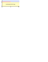
Figure 3: Regimes of biased diffusion in a piecewise linear random potential. At $f>g_{0}$ the normal biased diffusion occurs for all symmetric probability densities $u(g)$ with support on the interval $[-g_{0},g_{0}]$. A limiting case of subdiffusion, i.e., localization of particles at the average distance (3) from the origin, is realized at $f<g_{0}$. If $f=g_{0}$ then the character of diffusion depends on the exponent $\alpha$ characterizing the asymptotic behavior (37) of the residence time probability density $p(\tau)$. Specifically, normal diffusion occurs at $\alpha>2$ (dashed line) and anomalous one at $\alpha\in(0,2]$ (solid line). In turn, subdiffusion occurs if $\alpha\in(0,1/2)$, superdiffusion if $\alpha\in(1/2,1)$ or $\alpha\in(1,2)$, and other types of anomalous diffusion are realized at $\alpha=1/2$ (quasi-normal diffusion), $\alpha=1$ (weakened ballistic diffusion), and $\alpha=2$ (logarithmically enhanced normal diffusion).

We note in this context that all laws of diffusion were obtained within a single model dealing with the solution $X_{t}$ of the motion equation (2). In contrast, the CTRW jump model which deals with the discrete variable $Y_{t}$ reproduces only the long-time behavior of the variance $\sigma^{2}_{X}(t)$ if the waiting time is associated with the residence time DK . At short times the behavior of $\sigma^{2}_{X}(t)$ and $\sigma^{2}_{Y}(t)$ is completely different, see sections 4.

We complete our analysis of biased diffusion by comparing the root-mean-square displacement $\sigma_{X}(t)$ and the average displacement $\langle X_{t}\rangle$ at long times. Since $\sigma_{X}(t)$ characterizes the spreading of particles around their mean position $\langle X_{t}\rangle$, the coefficient of variation $C(t)=\sigma_{X}(t)/\langle X_{t}\rangle$ can be considered as a relative measure of the intensity of biased diffusion. Using the previous results, for normal diffusion we obtain $C(t)\propto 1/t^{1/2}$ ($t\to\infty$). In the case of anomalous diffusion the coefficient of variation at $\alpha\in[1,2]$ also tends to zero in the long-time limit, though more slowly than $1/t^{1/2}$. In particular, if $\alpha\in(1,2)$ then, according to (76) and (78), $C(t)\propto 1/t^{(\alpha-1)/2}$. In contrast, as follows from (69) and (71), the coefficient of variation $C(\infty)$ at $\alpha\in(0,1)$ does not vanish:

$$C(\infty)=\!\left(\frac{2\Gamma^{2}(1+\alpha)}{\Gamma(1+2\alpha)}-1\right)^{\!1/2}.$$ (91)

In this case the biased diffusion is so intensive that the spreading of particles is of the order of their displacement, i.e., $\sigma_{X}(t)\sim C(\infty)\langle X_{t}\rangle$. Interestingly, since $C(\infty)\to 0$ as $\alpha\to 1$ and $C(\infty)\to 1$ as $\alpha\to 0$, the slower the diffusion, the larger its intensity.

6 Conclusions

We have studied the unidirectional transport of particles which occurs under a constant external force in a piecewise linear random potential. The slopes of this potential, i.e., realizations of the piecewise constant random force, are assumed to be independent on different intervals of a fixed length and distributed with the same probability density. Using the overdamped motion equation, we have derived the probability density of the particle position and have calculated its first two moments by the Laplace transform method. The Laplace transforms of these moments are represented by means of the probability density of the residence time, i.e., time that a particle spends moving on the interval of a fixed length, which in turn is explicitly expressed through the probability density of the random force.

It has been shown that if the external force is less than the upper bound of the random force then the limiting case of subdiffusion, i.e., particle localization, occurs. In this regime, we have calculated the average distance between the origin and the points of localization which is always finite. In contrast, if the external force exceeds the upper bound of the random force then particles can be transported to an arbitrary large distance. Because of the influence of the random force, in this case the unidirectional motion of particles has a diffusive character. We have shown by applying the ordinary Tauberian theorem for the Laplace transform that at small times the biased diffusion is always ballistic. For the analysis of the transport properties at long times we used the modified Tauberian theorem that in most cases permits us to find the two leading terms of the asymptotic expansion of the first and second moments of the particle position. Within this approach, we have shown that the biased diffusion is normal and the diffusion coefficient as a function of the external force can be either monotonic or non-monotonic. The latter occurs if the probability density of the random force is concentrated near the edges of the interval of support.

If the external force is equal to the boundary value of the random force then at short times the biased diffusion remains ballistic, but at long times it can be either normal or anomalous. In the last case the character of diffusion depends on the asymptotic behavior of the probability density of the residence time, which is described by the exponent $\alpha$. Using the modified Tauberian theorem, it has been shown that at $\alpha\in(0,2]$ the biased diffusion is anomalous. Specifically, subdiffusion, i.e., power-law dependence of the variance on time with power less than 1 occurs at $\alpha\in(0,1/2)$, and superdiffusion, i.e., power-law dependence of the variance on time with power greater than $1$ occurs at $\alpha\in(1/2,1)$ and $\alpha\in(1,2)$. The quasi-normal diffusion, which is characterized by the nonlinear time dependence of the first moment of the particle position and the linear dependence of the variance, is realized at $\alpha=1/2$. Finally, the weakened ballistic diffusion and the logarithmically enhanced normal diffusion are realized at $\alpha=1$ and $\alpha=2$, respectively.

References

- (1) J.P. Bouchaud, A. Georges, Phys. Rep. 195, 127 (1990)
- (2) S. Scheidl, Z. Phys. B 97, 345 (1995)
- (3) P. Le Doussal, V.M. Vinokur, Physica C 254, 63 (1995)
- (4) P.E. Parris, M. Kuś, D.H. Dunlap, V.M. Kenkre, Phys. Rev. E 56, 5295 (1997)
- (5) D.A. Gorokhov, G. Blatter, Phys. Rev. B 58, 213 (1998)
- (6) S.I. Denisov, W. Horsthemke, Phys. Rev. E 62, 3311 (2000)
- (7) A.V. Lopatin, V.M. Vinokur, Phys. Rev. Lett. 86, 1817 (2001)
- (8) C. Monthus, Lett. Math. Phys. 78, 207 (2006)
- (9) P. Reimann, R. Eichhorn, Phys. Rev. Lett. 101, 180601 (2008)
- (10) M.N. Popescu, C.M. Arizmendi, A.L. Salas-Brito, F. Family, Phys. Rev. Lett. 85, 3321 (2000)
- (11) L. Gao, X. Luo, S. Zhu, B. Hu, Phys. Rev. E 67, 062104 (2003)
- (12) D.G. Zarlenga, H.A. Larrondo, C.M. Arizmendi, F. Family, Phys. Rev. E 75, 051101 (2007)
- (13) S.I. Denisov, T.V. Lyutyy, E.S. Denisova, P. Hänggi, H. Kantz, Phys. Rev. E 79, 051102 (2009)
- (14) H. Kunz, R. Livi, A. Sütő, Phys. Rev. E 67, 011102 (2003)
- (15) S.I. Denisov, M. Kostur, E.S. Denisova, P. Hänggi, Phys. Rev. E 75, 061123 (2007)
- (16) S.I. Denisov, M. Kostur, E.S. Denisova, P. Hänggi, Phys. Rev. E 76, 031101 (2007)
- (17) S.I. Denisov, H. Kantz, Phys. Rev. E 81, 021117 (2010)
- (18) E.W. Montroll, G.H. Weiss, J. Math. Phys. 6, 167 (1965)
- (19) B.D. Hughes, Random Walks and Random Environments (Clarendon Press, Oxford, 1995), Vol. 2
- (20) D. ben-Avraham, S. Havlin, Diffusion and Reactions in Fractals and Disordered Systems (Cambridge University Press, Cambridge, 2000)
- (21) R. Metzler, J. Klafter, Phys. Rep. 339, 1 (2000)
- (22) G. Zaslavsky, Phys. Rep. 371, 461 (2002)
- (23) Anomalous Transport: Foundations and Applications, edited by R. Klages, G. Radons, I.M. Sokolov (Wiley-VCH, Berlin, 2008)
- (24) M.F. Shlesinger, B. West, J. Klafter, Phys. Rev. Lett. 58, 1100 (1987)
- (25) J. Masoliver, K. Lindenberg, G.H. Weiss, Physica A 157, 891 (1989)
- (26) G. Zumofen, J. Klafter, Phys. Rev. E 47, 851 (1993)
- (27) E. Barkai, Chem. Phys. 284, 13 2002
- (28) I.M. Sokolov, R. Metzler, Phys. Rev. E 67, 010101(R) (2003)
- (29) V. Zaburdaev, M. Schmiedeberg, H. Stark, Phys. Rev. E 78, 011119 (2008)
- (30) W. Feller, An Introduction to Probability Theory and its Applications (Wiley, New York, 1971), Vol. 2
- (31) B.V. Gnedenko, V.Yu. Korolev, Random Summation: Limit Theorems and Applications (CRC Press, Boca Raton, FL, 1996)
- (32) A. Erdélyi, Tables of Integral Transforms (McGraw-Hill, New York, 1954), Vol. 1
- (33) M. Abramowitz, I.A. Stegun, Handbook of Mathematical Functions (Dover, New York, 1972)
- (34) M.F. Shlesinger, J. Stat. Phys. 10, 421 (1974)