The Bulk Channel in Thermal Gauge Theories

Abstract:

We investigate the thermal correlator of the trace of the energy-momentum tensor in the SU(3) Yang-Mills theory. Our goal is to constrain the spectral function in that channel, whose low-frequency part determines the bulk viscosity. We focus on the thermal modification of the spectral function, $\rho(\omega,T)-\rho(\omega,0)$. Using the operator-product expansion we give the high-frequency behavior of this difference in terms of thermodynamic potentials. We take into account the presence of an exact delta function located at the origin, which had been missed in previous analyses. We then combine the bulk sum rule and a Monte-Carlo evaluation of the Euclidean correlator to determine the intervals of frequency where the spectral density is enhanced or depleted by thermal effects. We find evidence that the thermal spectral density is non-zero for frequencies below the scalar glueball mass $m$ and is significantly depleted for $m\lesssim\omega\lesssim 3m$.

1 Introduction

Understanding the emergence of bulk properties and collective behavior from the strong interaction of particle physics is a goal that has been pursued vigorously in recent years. Experimentally, heavy-ion collisions have provided a way to heat up nuclear matter to temperatures at which quarks and gluons are expected to dominate its macroscopic properties [1, 2, 3, 4]. Theoretically, both analytic [5] and numerical methods [6] are being used to unravel the intricate dynamics of QCD at finite temperature and baryon density.

At temperatures of a few hundred MeV and small baryon density, lattice QCD remains the tool of choice to determine the equilibrium properties of the system. As we shall discuss in detail, access to the near-equilibrium properties, such as the transport properties, is limited in this approach, because lattice QCD employs the Euclidean formulation of thermal field theory. Real-time properties can thus only be determined by analytic continuation, which for numerical purposes represents an ill-posed problem. However, it is not excluded that we can learn about the gross features of the spectral density by suitably combining numerical and analytic methods. The purpose of this paper is to illustrate how such a combination of methods can be put to practice, taking as an example the bulk channel in the SU(3) Yang-Mills theory.

One of the lasting legacies of the Relativistic Heavy Ion Collider (RHIC) experiments is the success of the hydrodynamic description of the collisions, see for instance the review [7]. The early agreement between ideal hydrodynamics and experiment was gradually refined to incorporate the dissipative effects of shear viscosity $\eta$, the three-dimensional geometry [8, 9, 10] and to estimate the sensitivity to initial conditions [11, 12]. Most recently, the effects of bulk viscosity $\zeta$ have been investigated [13, 14]. At temperatures sufficiently high for weak coupling methods to be applicable, the bulk viscosity is three orders of magnitude smaller than the shear viscosity [15]. However, by analogy with many condensed matter systems (see for instance [16]), where a maxixum in the bulk viscosity is observed near liquid-gas phase transitions, one generally expects the bulk viscosity to become appreciable, if anywhere, near the rapid crossover between the confined and the deconfined phases. It has been suggested that this sudden onset of dissipation under expansion could trigger the freeze-out in heavy-ion collisions due to cavitation [14]; the breakup of a fluid occurs when a component of the stress-energy tensor, say $T_{zz}$, turns negative. The behavior of $\zeta$ near the QCD crossover was studied about two-and-a-half years ago, first using a QCD sum rule and a crude model for the bulk spectral function [17, 18], and subsequently using Euclidean correlators obtained by Monte-Carlo methods [19]. Both types of analyses missed the fact that a homogeneous fluctuation in $T_{\mu\mu}$ has a component which takes arbitrarily long to relax to equilibrium. It is therefore necessary to revisit these analyses, and this constitutes the second motivation for this work. A study based on AdS/CFT methods [20] also found an increase in the bulk viscosity near $T_{c}$, however less pronounced than suggested by [17, 19].

In the near future, the low-energy runs at RHIC, and further ahead, the heavy-ion experiments at FAIR will explore the QCD diagram at larger net baryon density. It is widely thought, although not beyond doubt, that a chiral critical point exists in the $T$ vs. $\mu_{B}$ plane [21]. The associated critical exponents [22] indicate that the bulk viscosity should exhibit a strong divergence near the critical point. If this increase in $\zeta$ is not too closely localized around $T_{c}$, it could be one of the signatures of the critical point.

The outline of this paper is as follows. We start in section 2 with a review of retarded and Euclidean correlators, establishing the precise relations between them. Details are collected in the appendix. In section (3) we turn to the specific case of the bulk channel in the SU($N$) gauge theory. We describe how to use the bulk sum rule as a constraint on the vacuum-subtracted spectral density $\Delta\rho$, and present the operator product expansion (OPE) prediction for the large-frequency behavior of the spectral density. In section 4 we give a numerical application of our results for $N=3$. We first present data deep in the confined phase, as well as in the deconfined phase. The sum rule is combined with lattice data to yield information on the changes in the spectral density that occur between the confined and the deconfined phases. We end with the conclusions of this study.

2 A review of finite-temperature correlators

In this section, we give the definitions of the retarded correlator and the Euclidean correlator, and show their relation in detail. This allows us to fix our conventions, but also to highlight a subtlety that arises in the zero-frequency case. The retarded correlator, evaluated at a purely imaginary frequency, is the analytic continuation of the Euclidean correlator, which is only available at the Matsubara frequencies. We show that the odd derivatives of the retarded correlator along the imaginary axis, evaluated at the origin, coincide with the derivatives of the spectral density at the origin. The even derivatives, on the other hand, correspond to integrals over all frequencies of the spectral density. We illustrate the relations that we derive on the example of the bulk channel in SU($N$) gauge theory. Working in frequency space rather than in time-coordinate space, we show the relation between the bulk viscosity and the frequency-space Euclidean correlator, Fig. (1).

We work in the canonical ensemble, i.e. expectation values of operators are defined by

$$\langle\hat{\cal O}\rangle=\frac{1}{Z}{\rm tr}\{e^{-\beta\hat{H}}\,\hat{\cal O}\},$$ (1)

where the partition function $Z(\beta)$ is such that $\langle 1\rangle=1$ and $\beta=1/T$ is the inverse temperature. In the following we consider a generic Hermitian operator ${\cal O}$. We use the Heisenberg representation, with

$$\hat{\cal O}(t)\equiv e^{i\hat{H}t}\hat{\cal O}(0)e^{-i\hat{H}t}\,.$$ (2)

We start by introducing the real-time correlators,

$$G_{R}(t)=i\theta(t)\langle[\hat{\cal O}(t),\hat{\cal O}(0)]\rangle\,.$$ (3)

Its Fourier transform

$$\tilde{G}_{R}(\omega)=i\int_{0}^{\infty}dt\,e^{i\omega t}\langle[\hat{\cal O}(t),\hat{\cal O}(0)]\rangle.$$ (4)

plays an important role in the following. With these conventions we note that $\tilde{G}_{R}$ is analytic in the half complex plane $\mathop{\rm Im}(\omega)>0$.

The Euclidean correlator is defined as

$$G_{E}(t)=\langle\hat{\cal O}(-it)\,\hat{\cal O}(0)\rangle.$$ (5)

It obeys the Kubo-Martin-Schwinger relation

$$G_{E}(\beta-t)=G_{E}(t)\,,$$ (6)

and can be expressed as a Fourier series on the interval $0\leq t<\beta$,

$$G_{E}(t) = T\sum_{\ell\in{\bf Z}}G_{E}^{(\ell)}\,e^{i\omega_{\ell}t}\,,$$ (7)

$$G_{E}^{(\ell)} = \int_{0}^{\beta}dte^{-i\omega_{\ell}t}G_{E}(t)\,,$$ (8)

where $\omega_{\ell}=\omega_{M}\cdot\ell=2\pi T\,\ell$.

The spectral representation of the correlators is useful to prove simple relations between the Euclidean and real-time correlators. One finds that (see the appendix)

$$G_{R}(i\omega_{\ell})=G_{E}^{(\ell)}\,,\quad\ell\neq 0\,.$$ (9)

The relation of the Matsubara zero-mode $\ell=0$ with the zero-frequency retarded correlator requires special care. We shall see that their difference can be expressed in terms of the spectral function.

The spectral function is defined as

$$\rho(\omega)=\frac{1}{\pi}\mathop{\rm Im}\tilde{G}_{R}(\omega)\,.$$ (10)

For real $\omega$ and in finite volume, $\rho$ is a distribution, namely a discrete sum of delta functions. However, in the infinite-volume limit of an interacting theory, it is typically a smooth function, except possibly at a finite number of points. The most useful relations among the correlators are those that survive the infinite-volume limit. In the appendix, we show that

$$G_{E}^{(0)}-\tilde{G}_{R}(i\omega_{I})=\lim_{\Lambda\to\infty}\int_{-\Lambda}^{\Lambda}\frac{d\omega}{\omega}\,\rho(\omega)\,\frac{\omega_{I}^{2}}{\omega^{2}+\omega_{I}^{2}}\,,~{}~{}~{}\forall\omega_{I}>0.$$ (11)

In the limit $\omega_{I}\to 0$, only the integration region around the origin contributes on the RHS. If the spectral function is finite at the origin, the RHS is O($\omega_{I}$), and therefore $\lim_{\epsilon\to 0}\tilde{G}_{R}(i\epsilon)=G_{E}^{(0)}$. On the other hand, if the spectral function contains a delta-function at the origin, $\rho(\omega)/\omega=A\delta(\omega)$, $\lim_{\epsilon\to 0}\tilde{G}_{R}(i\epsilon)=G_{E}^{(0)}-A$. We have written Eq. (11) with an explicit UV cutoff to make it clear that one should take the limit $\omega_{I}\to 0$ first.

The connection between the retarded and Euclidean correlators is thus precisely established in frequency space. In appendix we also rederive the relation between them in coordinate space (well-known in particular to lattice practitioners),

$$G_{E}(t)=\int_{0}^{\infty}d\omega\rho(\omega)\frac{\cosh\omega(\frac{\beta}{2}-t)}{\sinh\beta\omega/2}\,,$$ (12)

which we shall use in section (4).

2.1 The retarded correlator along the imaginary axis

If we assume for a moment that

$$\int_{C}^{\infty}\rho(\omega)\frac{d\omega}{\omega},\qquad(C>0),$$ (13)

converges in the UV, a simple calculation based on the explicit expression for the spectral density (92), or alternatively a contour integration, then leads to the Kramers-Kronig relation

$$\int_{-\infty}^{+\infty}d\omega\,\rho(\omega)\frac{\omega}{\omega^{2}+\omega_{\rm I}^{2}}=\tilde{G}_{R}(i\omega_{\rm I})\,,\qquad\forall\omega_{\rm I}>0.$$ (14)

In general, it is necessary to perform a subtraction from $\rho$ to make the dispersion integral converge in quantum field theory. Starting from (14), it is easy to derive by recursion the following equalities,

$$(-1)^{n}\frac{d^{2n}}{d\omega_{\rm I}^{2n}}\tilde{G}_{R}(i\omega_{\rm I}) = \int_{-\infty}^{\infty}d\omega\rho^{(2n)}(\omega)\,\frac{\omega}{\omega^{2}+\omega_{\rm I}^{2}}$$ (15)

$$(-1)^{n+1}\frac{d^{2n+1}}{d\omega_{\rm I}^{2n+1}}\tilde{G}_{R}(i\omega_{\rm I}) = \int_{-\infty}^{\infty}d\omega\rho^{(2n+1)}(\omega)\frac{\omega_{\rm I}}{\omega^{2}+\omega_{\rm I}^{2}}\stackrel{{\scriptstyle\omega_{I}\to 0}}{{=}}\pi\rho^{(2n+1)}(\omega=0)\,.$$ (16)

Thus at the origin, the even derivatives of the retarded correlator along the imaginary axis are given by integrals over the spectral density, while the odd derivatives are equal to the corresponding derivatives of the spectral function.

2.2 Remarks on the Euclidean correlator

Combining Eq. (14) with Eq. (11), one obtains

$$G_{E}^{(0)}=\int_{-\infty}^{\infty}d\omega\,\frac{\rho(\omega)}{\omega}\,.$$ (17)

Equations (11) and (17) show that while $G_{R}(i\omega_{\rm I})$ is insensitive to the presence of a $\omega\delta(\omega)$ term in the spectral function for any $\omega_{\rm I}>0$, $G_{E}^{(0)}$ definitely receives a contribution from it.

Secondly we remark that the positivity of $\rho(\omega)/\omega$ implies the positivity of certain linear combinations of the Euclidean correlator. For instance,

$$G_{E}^{(0)}-G_{E}^{(\ell)} = \omega_{\ell}^{2}\int_{-\infty}^{\infty}d\omega\,\frac{\rho(\omega)}{\omega}\,\frac{1}{\omega^{2}+\omega_{\ell}^{2}}\,,$$ (18)

$$3G_{E}^{(0)}-4G_{E}^{(\ell)}+G_{E}^{(2\ell)} = 12\omega_{\ell}^{4}\int_{-\infty}^{\infty}d\omega\frac{\rho(\omega)}{\omega}\,\frac{1}{(\omega^{2}+\omega_{\ell}^{2})(\omega^{2}+4\omega_{\ell}^{2})}\,.$$ (19)

2.3 An example

Here we anticipate the results of section (3) to illustrate the general formulas of this section. In Figure (1), we sketch a possible form of the retarded correlator for the operator $T_{\mu\mu}$ projected onto zero spatial momentum. In order to deal with a UV finite function, we subtract the corresponding zero-temperature correlator,

$$\Delta\tilde{G}_{R}(i\omega)=\tilde{G}_{R}(i\omega,T)-\tilde{G}_{R}(i\omega,T=0)$$ (20)

and leave the temperature-dependence implicit. This subtraction is sufficient to make the dispersion integral (14) converge. As we shall see in section (3.1), the spectral function of the operator $\int d^{3}{\bf x}\,T_{\mu\mu}(x)$ admits a delta function located at the origin, with a weight given by a thermodynamic quantity. Applying Eq. (11), we obtain $\Delta\tilde{G}_{R}(i\epsilon)=\Delta G_{E}^{(0)}-Tc_{v}(3c_{s}^{2}-1)^{2}$. Furthermore an exact sum rule fixes $\Delta G^{(0)}_{E}$ in terms of thermodynamic functions, and $\Delta\tilde{G}_{R}(i\epsilon)$ turns out to be negative. Using the operator-product expansion (section 3.2), one can show that $\Delta G_{E}^{(\ell)}$ is negative at large Matsubara frequencies, implying the same for $\Delta\tilde{G}_{R}(i\omega)$ at large $\omega$ in view of Eq. (9). Finally, Eq. (16) and (30) show that $(d/d\omega)\Delta\tilde{G}_{R}(i\omega)$ at the origin is proportional to the bulk viscosity, which has to be positive by the second law of thermodynamics. All this information is summarized in Fig. (1). The behavior at intermediate frequencies $\omega$ is not known to us, in principle $\Delta\tilde{G}_{R}(i\omega)$ could even change sign in view of the subtraction made. It is also not known whether the plotted function ever exceeds unity for $\omega$ a multiple of $2\pi T$.

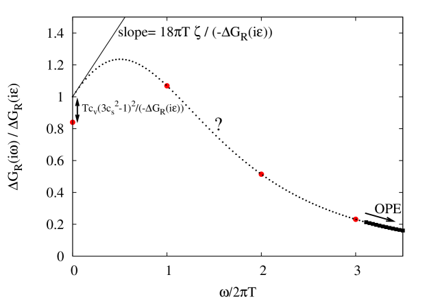
Figure 1: A sketch of the retarded correlator for the operator $L^{-3/2}\int d^{3}{\bf x}T_{\mu\mu}(x)$ at purely imaginary frequencies (dotted line). The large dots indicate the values of $\Delta G_{E}^{(\ell)}$, calculable in the Euclidean theory. Figure (2) shows that $\Delta\tilde{G}_{R}(i\epsilon)=3(e+p)(1-3c_{s}^{2})-4(e-3p)$ is negative in the deconfined phase. At high frequencies, $\Delta\tilde{G}_{R}$ is constrained by the OPE.

In a numerical Euclidean approach, the available information is $\tilde{G}_{R}(i\omega_{\ell})$, $\ell=0,1,\dots$ The low-frequency real-time properties of the system, such as the bulk viscosity and the associated relaxation time, are determined by the odd derivatives of $\tilde{G}_{R}(i\omega)$ at the origin, see Eq. (16). The latter are difficult to determine, because $\omega=0$ is a non-analytic point of $\tilde{G}_{R}$. In this respect, Eq. (16) shows that if the spectral density has a gap $m$, as it does at zero temperature in a confining theory, then $\tilde{G}_{R}(i\omega)$ can be expanded in integer powers of $\omega^{2}$. Therefore subtracting the zero-temperature correlator only affects the even derivatives of $\Delta\tilde{G}_{R}(i\omega)$ at the origin.

Working in frequency space has the advantage that the high-frequencies are decoupled from the discussion at this stage. There are, however, technical difficulties in determining Euclidean correlators in frequency space. Unlike the $t$-dependent correlators, they are off-shell correlators, and therefore require additive counterterms in order to approach the continuum limit with corrections that are suppressed with a power of the lattice spacing. An example of this complication arises in the derivation of sum rules [23]. In this special case the sum rule precisely dictates what the counterterms are. In general, renormalization conditions have to be imposed in order to determine them.

Finally we make the observation that a polynomial of degree $n$ in $\omega$ going through the $n+1$ points $\{\tilde{G}_{R}(i\epsilon)\}\cup\{G_{E}^{(\ell)}\}_{\ell=1}^{n}$, has a slope at the origin given by

$$-\frac{n!}{\omega_{M}}\sum_{\ell=1}^{n}\frac{(-1)^{\ell}}{\ell!(n-\ell)!}\frac{G_{E}^{(\ell)}-\tilde{G}_{R}(i\epsilon)}{\ell}\,.$$ (21)

When expressed in terms of dispersion integrals as in Eq. (18-19), the degree of convergence in the UV of this expression improves with the order of the polynomial: with some combinatorics one can show that it is asymptotically $\rho(\omega)/\omega^{n+3}$ for $n$ even and $\rho(\omega)/\omega^{n+2}$ for $n$ odd. In particular, the slope at the origin of the $n=2$ polynomial is given by

$$-\frac{1}{2\omega_{M}}(3\tilde{G}_{R}(i\epsilon)-4G_{E}^{(1)}+G_{E}^{(2)})=-6\omega_{M}^{3}\int_{-\infty}^{\infty}d\omega\,\frac{\rho(\omega)\omega}{\omega^{2}+\epsilon^{2}}\frac{1}{(\omega^{2}+\omega_{M}^{2})\,(\omega^{2}+4\omega_{M}^{2})}\,,$$ (22)

where the linear combination (19) appears. In the specific case of the bulk channel, the spectral integral (22) is UV-convergent without any subtraction to $\rho(\omega)$. Thus the slope of the quadratic polynomial is negative-definite, just as the actual slope of the retarded correlator $\frac{d}{d\omega}\tilde{G}_{R}(i\omega)$. One might be tempted to use it as a Euclidean estimator for the bulk viscosity $\zeta$. However, if the spectral function has a transport peak at the origin of width $\omega_{0}\lesssim\omega_{M}$, expression (22) amounts parametrically to $\zeta\omega_{0}/\omega_{M}$, while $\frac{d}{d\omega}\tilde{G}_{R}(i\omega)\sim\zeta$. It is clear why that is: a polynomial interpolating between the Euclidean points is only a good approximation to the retarded correlator if the latter does not contain a scale $\omega_{0}\ll\omega_{M}$ over which it varies significantly.

2.4 The reconstructed Euclidean correlator

When analyzing Euclidean correlators obtained from Monte-Carlo simulations, it is instructive to study in what way the Euclidean correlators differ from what they would be if the spectral density was unaffected by thermal effects [24]:

$$G_{E}^{\rm rec}(t,T;T^{\prime}){\equiv}\int_{0}^{\infty}d\omega\rho(\omega,T^{\prime})\frac{\cosh\omega(\frac{\beta}{2}-t)}{\sinh\omega\beta/2}\,.$$ (23)

The identity ($0\leq t\leq\beta$)

$$\frac{\cosh\omega(\frac{\beta}{2}-t)}{\sinh\omega\beta/2}=\sum_{m\in{\bf Z}}e^{-\omega|t+m\beta|}$$ (24)

allows us to derive in particular the exact relations

$$G_{E}^{\rm rec}(t,T;0) = \sum_{m\in{\bf Z}}G_{E}(|t+m\beta|,T=0)\,,$$ (25)

$$G_{E}^{\rm rec}(t,T;{\textstyle\frac{1}{2}}T) = G_{E}(t,{\textstyle\frac{1}{2}}T)+G_{E}(\beta-t,{\textstyle\frac{1}{2}}T)\,.$$ (26)

These expressions are useful in practice when one is interested in a difference of spectral functions. We will exploit Eq. (25). Even if the zero-temperature Euclidean correlator can usually not be determined for arbitrarily large separations, in that regime it is completely dominated by the lightest state in the channel, so that its functional form is known and completely determined by one matrix element and an energy. The contribution to $G_{E}^{\rm rec}$ of a single state of energy $E$ is easily obtained,

$$\delta G_{E}^{\rm rec}(t,T)\sim\frac{\cosh E(\beta/2-t)}{\sinh\beta E/2}\,.$$ (27)

Secondly, the correlator falls off very rapidly, so that the terms with large values of $m$ in Eq. (25) make a very small contribution.

3 The bulk channel in QCD

In this section the goal is to provide the theoretical background for the analysis of the bulk channel in SU($N$) gauge theory. Thus we consider the operator

$${\cal O}_{\theta}(t)=\frac{1}{L^{3/2}}\int d^{3}{\bf x}~{}\theta(t,{\bf x})\,,\qquad\theta(x)\equiv T_{\mu\mu}(x)={\textstyle\frac{\beta(g)}{2g}}G_{\mu\nu}^{a}(x)G_{\mu\nu}^{a}(x)\,.$$ (28)

Here $\beta(g)$ is the beta function, $\beta(g)=-bg^{3}+\dots$, $b=\frac{11N}{3(4\pi)^{2}}$, and $T_{\mu\nu}(x)$ is the energy-momentum tensor. Its spectral function $\rho_{\theta}(\omega,T)$ and the difference

$$\Delta\rho_{\theta}(\omega,T)\equiv\rho_{\theta}(\omega,T)-\rho_{\theta}(\omega,0)$$ (29)

play an important role in the following. The spectral function determines the bulk viscosity through the Kubo formula

$$\zeta(T)=\frac{\pi}{9}\lim_{\omega\to 0}\frac{\rho_{\theta}(\omega)}{\omega}.$$ (30)

In what follows we review the behavior that hydrodynamics predicts for the low-frequency part of the associated spectral function $\rho_{\theta}$. It turns out that it contains a term $\omega\delta(\omega)$. We then define an ‘auxiliary’ operator whose spectral function coincides with $\rho_{\theta}$ except for not having the delta function at the origin. Next we present the asymptotic large-$\omega$ behavior of $\rho_{\theta}$ based on the operator-product expansion. Finally, the spectral function of the auxiliary operator obeys a sum rule given in section (3.2).

3.1 Low-frequency prediction from hydrodynamics

In this section we consider more general connected correlation functions of the energy-momentum tensor,

$$G_{E,\mu\nu\rho\sigma}(t,{\bf k})=\int d^{3}{\bf x}\,e^{i{\bf k\cdot x}}\,\langle T_{\mu\nu}(t,{\bf x})\,T_{\rho\sigma}(0)\rangle\,,$$ (31)

as well as their associated spectral function $\rho_{\mu\nu\rho\sigma}(\omega,{\bf k},T)$ via (12). The spectral function for $T_{33}$ (assuming the spatial momentum ${\bf k}$ is pointing in the direction $\hat{3}$) reads [25]

$$\frac{\rho_{33,33}(\omega,{\bf k},T)}{\omega}=\frac{e+p}{\pi}\frac{\Gamma_{s}\omega^{4}}{(\omega^{2}-c_{s}^{2}k^{2})^{2}+(\Gamma_{s}\omega k^{2})^{2}}.$$ (32)

Now one shoud recall that for any smooth function such that $\int_{-\infty}^{\infty}f(x)dx=1$, $\frac{1}{\epsilon}f(x/\epsilon)$ provides a representation of the delta function. Here we will exploit this fact for the function

$$f(x)=\frac{1}{\pi(b^{2}-1)}\left[\frac{x^{4}}{(x^{2}-b^{2})^{2}+x^{2}}-1\right]$$ (33)

and $b=c_{s}/(\Gamma_{s}k)$ and $\epsilon=\Gamma_{s}k^{2}$. In this way one finds that, in the sense of distributions,

$$\lim_{{\bf k}\to 0}\frac{\rho_{33,33}(\omega,{\bf k},T)}{\omega}=\frac{e+p}{\pi}\Gamma_{s}+(e+p)c_{s}^{2}\delta(\omega)+\dots$$ (34)

This is in contrast with what is obtained if one simply sets ${\bf k}=0$ in Eq. (32), in which case one misses the delta function. In the shear channel on the other hand,

$$\frac{\rho_{13,13}(\omega,{\bf k},T)}{\omega}=\frac{\eta}{\pi}\frac{\omega^{2}}{\omega^{2}+\left(\frac{\eta k^{2}}{e+p}\right)^{2}}\stackrel{{\scriptstyle{\bf k}\to 0}}{{\sim}}\frac{\eta}{\pi}-\frac{\eta^{2}k^{2}}{e+p}\delta(\omega)$$ (35)

and the delta function is suppressed by a power of ${\bf k}^{2}$. Thus combining the shear and sound channels,

$$\frac{1}{9}\frac{\rho_{ii,kk}(\omega,{\bf 0},T)}{\omega}=\frac{\rho_{33,33}(\omega,{\bf 0},T)}{\omega}-\frac{4}{3}\frac{\rho_{13,13}(\omega,{\bf 0},T)}{\omega}=\frac{\zeta}{\pi}+(e+p)c_{s}^{2}\delta(\omega)+\dots$$ (36)

Using the exact relations

$$\rho_{00,00}(\omega,{\bf 0},T) = \frac{e+p}{c_{s}^{2}}\omega\delta(\omega)\,,$$ (37)

$$\rho_{00,kk}(\omega,{\bf 0},T) = -3(e+p)\omega\delta(\omega)\,,$$ (38)

one finds

$$\frac{\rho_{\theta}(\omega,{\bf 0},T)}{\omega}\equiv\frac{\rho_{\mu\mu,\nu\nu}(\omega,{\bf 0},T)}{\omega}=\frac{9\zeta}{\pi}+\frac{e+p}{c_{s}^{2}}(3c_{s}^{2}-1)^{2}\delta(\omega)+\dots$$ (39)

When one constrains the spectral function using sum rules and Euclidean correlators, one is always dealing with integrals of the spectral function over all frequencies. Therefore it is useful to subtract the contribution of the delta function in (39). One way to achieve this is to work with the operator

$${\cal O}_{\star}=L^{-3/2}\int d^{3}{\bf x}\,\left(T_{\mu\mu}(x)+(3c_{s}^{2}-1)T_{00}(x)\right)\,.$$ (40)

Its spectral function, which we denote by $\rho_{\star}$, satisfies

$$\rho_{\theta}(\omega,{\bf 0},T)=\rho_{\star}(\omega,{\bf 0},T)+\frac{e+p}{c_{s}^{2}}(3c_{s}^{2}-1)^{2}\,\omega\,\delta(\omega)$$ (41)

and, in view of Eq. (39), is free of the delta function at the origin. At equilibrium, recalling that $c_{s}^{2}=\frac{\partial p}{\partial e}$,

$$-\frac{1}{3}\langle{\cal O}_{\star}\rangle=p-{\textstyle\frac{\partial p}{\partial e}}e$$ (42)

and therefore its linear fluctuations are not correlated with those of the total energy. This is the physical reason why a delta function at the origin is absent in its spectral function.

3.2 Large-frequency behavior from the operator product expansion

In section (3.1) we have analyzed the low-frequency behavior of the bulk spectral function using the general hydrodynamic predictions. We now turn to an analysis of its asymptotic high-frequency behavior. The leading $\rho_{\theta}\sim\alpha_{s}^{2}(\omega)\omega^{4}$ behavior was given for instance in [26]. In the OPE language, this contribution corresponds to the insertion of the unit operator, and it is therefore temperature independent. Because it makes a large contribution to the coordinate-space Euclidean correlator, it is best to remove it by subtracting the vacuum correlator from the thermal correlator. We therefore need to know what the leading behavior of the subtracted correlator and of the corresponding subtracted spectral function is.

The operator product expansion of local gluonic operators was calculated a long time ago in the context of QCD sum rules [27], and the results of more recent calculations are summarized in [28]. In many cases, the Wilson coefficients are known at next-to-leading order. However, only the Lorentz scalar operators were kept on the right-hand side of the OPE, since the correlator was evaluated in the vacuum. Since we want to apply the OPE to a system at finite-temperature, the traceless part of the energy-momentum tensor, for instance, can also contribute. The OPE results therefore need to be generalized to the finite-temperature context [29]. We have reproduced the result of [29] for the bulk channel using the background field method combined with the Fock-Schwinger gauge [30],

$$\Delta\rho_{\theta}(\omega,{\bf 0},T)\stackrel{{\scriptstyle\omega\to\infty}}{{\sim}}-\frac{1}{2}\left(\frac{11N\alpha_{s}(\omega)}{6\pi}\right)^{2}(e-3p)-\frac{3}{4}\left(\frac{11N\alpha_{s}(\omega)}{6\pi}\right)^{3}(e+p)\,.$$ (43)

We remark that while the two-point function $\Delta\tilde{G}_{R}(i\omega)$ of the operator $T_{\mu\nu}-\frac{1}{4}\delta_{\mu\nu}\theta$ contains a logarithmic divergence (which manifests itself in the Wilson coefficient of $\theta$ being O($1/g_{0}^{2}\sim\log 1/a$) in lattice regularization [23]), $\Delta\tilde{G}_{R}(i\omega)$ is UV-finite for the operator $\theta$. Therefore, assuming the validity of the operator-product expansion, the only relevant scale in its Wilson coefficients is $\omega$, and the dispersion relation (14) then leads to Eq. (43) [31]. In section (4), we will use this information to constrain the form of the spectral function at large frequencies.

3.3 The Bulk Sum Rule

The idea of constraining the form of finite-temperature spectral functions with sum rules is not new [32, 31, 17]. Here we focus on the bulk channel. In Euclidean space, the following sum rule holds [33],

$$G_{E,\theta}^{(0)}(T)-G_{E,\theta}^{(0)}(T=0)=T^{5}\frac{\partial}{\partial T}\frac{e-3p}{T^{4}}\,,$$ (44)

where $e$ and $p$ are the energy density and pressure of the finite-temperature system.

We now convert identity (44) into a sum rule for the bulk spectral function with the goal to constrain the latter. Combining equations (44) and (17), we obtain

$$\int_{-\infty}^{\infty}\frac{d\omega}{\omega}[\rho_{\theta}(\omega,T)-\rho_{\theta}(\omega,0)]=T^{5}\partial_{T}\frac{e-3p}{T^{4}}\,.$$ (45)

Next, we separate the contribution of the $\omega\delta(\omega)$ term in $\rho_{\theta}$ from the rest of the spectral function. In other words, we want to turn Eq. (45) into a sum rule for $\rho_{\star}$, the spectral function of the operator ${\cal O}_{\star}$ (40), which is smooth at the origin. Using Eq. (41), one finds

$$2\int_{0}^{\infty}\frac{d\omega}{\omega}[\rho_{\star}(\omega,T)-\rho_{\star}(\omega,0)]=3(1-3c_{s}^{2})(e+p)-4(e-3p)\,.$$ (46)

A few remarks are in order. It would have been less straightforward to directly derive a sum rule for $\rho_{\star}$, because the Euclidean correlator of ${\cal O}_{\star}$ contains a short-distance singularity. We remark that Eq. (45) was already obtained in [17], but the presence of the $\omega\delta(\omega)$ term in $\rho_{\theta}$ was missed. In [34], a finite spatial momentum ${\bf k}$ was used as an infrared regulator and the contribution of the zero-frequency delta function correctly identified for the first time. If one insists on expressing Eq. (46) in terms of $\rho_{\theta}$, one should strictly write $\lim_{\epsilon\to 0}\int_{-\infty}^{\infty}\frac{\omega\,d\omega}{\omega^{2}+\epsilon^{2}}\Delta\rho_{\theta}(\omega,T)=3(1-3c_{s}^{2})(e+p)-4(e-3p)$.

4 Numerical results from the lattice

In this section we describe the lattice setup and the numerical results obtained by Monte-Carlo simulations. We employ the isotropic Wilson action [35],

$$S_{\rm g}=\frac{1}{g_{0}^{2}}\sum_{x,\mu\neq\nu}{\rm tr}\{1-P_{\mu\nu}(x)\}\,,$$ (47)

where the ‘plaquette’ $P_{\mu\nu}$ is the product of four link variables $U_{\mu}(x)\!\in\,$SU(3) around an elementary cell in the $(\mu,\nu)$ plane. As a discretization of $L^{3/2}{\cal O}_{\theta}$, we use

$$a^{3}\sum_{\bf x}\Theta(x)=\frac{-2}{a}\frac{dg_{0}^{-2}}{d\log a}\sum_{\bf x}\mathop{\rm Re}{\rm tr}\Big{\{}{\textstyle\sum_{k}}P_{0k}(x)+{\textstyle\sum_{k<l}}\frac{1}{2}[P_{kl}(x)+P_{kl}(x+a\hat{0})]\Big{\}},$$ (48)

up to an irrelevant additive constant (its contribution vanishes in connected correlation functions). As a local update algorithm, we use the standard combination of heatbath and over-relaxation [36, 37, 38, 39] sweeps in a ratio increasing from 3 to 5 as the lattice spacing is decreased. The multi-level algorithm is used to reduce the variance of the correlator [40, 41]. To set the scale and to evaluate the lattice beta function $dg_{0}^{-2}/d\log a$ we use the parametrization of the Sommer scale $r_{0}\approx 0.5$fm given in [42]. We denote the mass gap by $m$, given by the lightest scalar glueball, whose mass is $3.96(5)/r_{0}=m=5.30(8)T_{c}$. Finally we relate the notation used in the rest of this section to the general definitions of sections (2) and (3),

$$C_{\theta}(t,T)\equiv\beta^{5}G_{E,\theta}(t), C_{\star}(t,T)\equiv\beta^{5}G_{E,\star}(t),$$ (49)

$$C^{\rm rec}_{\star}(t,T;T_{0})\equiv\beta^{5}G^{\rm rec}_{E,\star}(t,T;T_{0})\,, C^{\rm rec}_{\star}(t,T)\equiv C^{\rm rec}_{\star}(t,T;0)\,,$$ (50)

$$\Delta\rho_{\star}(\omega,T)=\rho_{\star}(\omega,T)-\rho_{\star}(\omega,0)\,.$$ (51)

The quantities with a $\star$ subscript are associated with the operator ${\cal O}_{\star}$ defined in Eq. (40). The Euclidean correlators $C_{\dots}$ are dimensionless, renormalization-group invariant quantities. The goal of this section is to constrain the function $\Delta\rho_{\star}$, the main results being Eq. (72) and Eq. (73).

We start by describing a method we have used to evaluate the right-hand side of the bulk sum rule (46). We also evaluate the ‘condensates’ appearing in the OPE (43) of the bulk correlator. We obtain $C_{\star}$ at finite temperature by subtracting the contribution of the $\delta$ function. We then describe the properties of the correlator at temperatures deep in the confined phase. This correlator is subsequently used to produce a ‘reconstructed’ correlator based on (25). From then on we are directly dealing with integrals of the subtracted spectral function, $\Delta\rho_{\star}$. We reuse lattice data presented in [19], and combine it with the bulk sum rule to determine the gross features of the bulk spectral function.

4.1 Right-hand side of the bulk sum rule

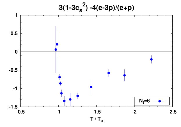
Figure 2: The right-hand side of the bulk sum rule as a function of temperature. The spatial volume in the finite-temperature simulations is typically $28^{3}$.

When using the bulk sum rule (46), the question arises, how to best evaluate the combination of thermodynamic quantities appearing on the right-hand side of the equation. Note that the enthalpy $e+p$ and the conformality measure $e-3p$ are relatively straightforward to obtain from the expectation value of the electric and magnetic field strengths. What is then needed is a reliable way to obtain the velocity of sound $c_{s}^{2}$, or alternatively, the specific heat $c_{v}$.

The Euclidean sum rule (44) can be derived on the lattice. Here we will use that lattice sum rule [23] to determine the velocity of sound via

$$\frac{1}{c_{s}^{2}}-3=\left(4-\frac{d^{2}g_{0}^{-2}/d(\log a)^{2}}{dg_{0}^{-2}/d\log a}\right)\frac{e-3p}{e+p}+\frac{a^{4}}{e+p}\sum_{x}\langle\Theta(x)\Theta(0)\rangle^{\rm conn}_{T-0}\,,$$ (52)

where the discretization $\Theta$ of the trace anomaly operator is given by Eq. (48). We used the leading perturbative expression for the expression inside the large brackets, since based on that estimate it only departs from 4 by 0.008 or less.

The right-hand side of the bulk sum rule (46), as calculated on $N_{\tau}=6$ lattices, is displayed in units of $e+p$ in Fig. (2) as a function of temperature. It is negative for a significant range of temperatures above $T_{c}$, and its leading behavior in perturbation theory is [43]

$$3(1-3c_{s}^{2})-4\frac{e-3p}{e+p}=-10\cdot\left({\textstyle\frac{11}{3}}\right)^{2}\cdot\left(\frac{\alpha_{s}N}{4\pi}\right)^{3}+\dots$$ (53)

It is therefore likely to be negative throughout the deconfined phase. We also note that for $\alpha_{s}=0.25$, the right-hand side of (53) amounts to about -0.03, a very small value compared to those appearing in Fig. (2).

4.2 Evaluation of the correlator $C_{\star}(t,T)$

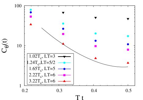
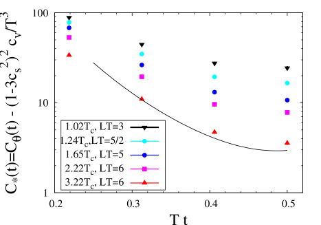
Figure 3: The treelevel-improved $C_{\theta}$ correlator for several temperatures. On the right panel, $\frac{c_{v}}{T^{3}}\,(1-3c_{s}^{2})^{2}$ has been subtracted.

Since we want to work with the correlation functions of the operator ${\cal O}_{\star}$, we have to evaluate its Euclidean correlation function $C_{\star}(t)$. Lattice perturbation theory [44] and numerical studies [19] show that it is advantageous to work with the operator ${\cal O}_{\theta}$. To convert its correlation function to the correlation function $C_{\star}$, we use the equation (see 41 and 12)

$$C_{\theta}(t,T)=C_{\star}(t,T)+\frac{e+p}{T^{4}c_{s}^{2}}(3c_{s}^{2}-1)^{2}\,.$$ (54)

Here too a combination of thermodynamic quantities appears. We have obtained it by the same method as the right-hand side of the bulk sum rule, see the previous subsection. Close to the phase transition where $c_{s}^{2}$ is very small, the result is rather sensitive to the value of $c_{s}^{2}$, since it appears in the denominator. That is the main reason we opted for a direct calculation of $c_{s}^{2}$ from the lattice sum rule (52), rather than parametrizing the pressure and obtaining $c_{s}^{2}$ by taking derivatives. In this way we avoid the dependence on a parametrization ansatz, which can be significant in a region where the derivatives are very large. On the other hand, at high temperatures

$$\frac{1}{c_{s}^{2}}(3c_{s}^{2}-1)^{2}=100\cdot\left({\textstyle\frac{11}{3}}\right)^{2}\cdot\left(\frac{N\alpha_{s}}{4\pi}\right)^{4}+\dots$$ (55)

and the difference between $C_{\theta}$ and $C_{\star}$ is parametrically negligible, since both are O($\alpha_{s}^{2}$).

The resulting correlators are displayed in Fig. (3). The lattice data for $C_{\theta}$ is the same as in [19]. In particular, the lattice spacing is given by $1/aT=8$. At high temperatures, there is very little numerical difference between them, confirming the parametric expectation (55). On the other hand we observe that the difference between $C_{\theta}$ and $C_{\star}$ becomes appreciable very close to $T_{c}$. At that point, $C_{\star}$ is significantly smaller than $C_{\theta}$.

4.3 Low-temperature correlators

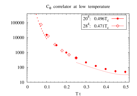
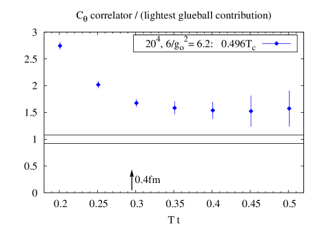
Figure 4: The $\theta$ correlator at about half the deconfining temperature. The leading-order perturbative prediction, with $\alpha_{s}=0.30$, appears at small $t$. The contribution of the lightest scalar glueball is given at larger $t$. On the right panel, the correlator has been divided by the contribution of the lightest scalar glueball. Treelevel improvement has not been applied.

The $C_{\theta}$ correlator at about $T_{c}/2$ is displayed in Fig. (4). The agreement between the data obtained at two different lattice spacings suggests that the cutoff effects on the correlators are small. The dotted curve at small separation, which represents the leading perturbative prediction for the choice $\alpha_{s}=0.30$, shows that by comparison the non-perturbative correlator is rather large. The right panel shows that starting at about 0.4fm, the lightest glueball represents a large contribution of the full correlator. The data is not accurate enough to tell how well that state saturates the correlator beyon 0.6fm.

Although the finite size of the lattice implies that the temperature is about $T_{c}/2$, rather than zero, it is very likely that the spectral function is already close to the zero-temperature spectral function, albeit in finite volume. This statement can be justified as follows. The confined phase can be thought of as a dilute gas of glueballs propagating freely, up to occasional collisions. Evidence in favor of this picture comes from a precision thermodynamic calculation in the confined phase [45]. Thus, to leading order at low temperatures,

$$s(\beta) \approx m\beta\left(\frac{m}{2\pi\beta}\right)^{3/2}\,\exp(-\beta m)$$ (56)

$$c_{v} \approx (\beta m)s(\beta)\,,$$ (57)

where $m$ is the mass gap. Based on these approximate expressions, we find that the contribution of the exact delta function to the correlator $C_{\theta}$ at $t=\beta/2$ is

$$\left[C_{\theta}(t,T)-C_{\star}(t,T)\right]_{t=\beta/2}\simeq(\beta m)^{2}\left(\frac{m\beta}{2\pi}\right)^{3/2}e^{-\beta m}\,.$$ (58)

Numerically, at $T=T_{c}/2$ this evaluates to about $0.006$, while $C_{\theta}(T,\beta/2)=50(11)$. The area under the transport peak can be estimated using kinetic theory. The general expression is given in [25],

$$\int_{-\Lambda}^{\Lambda}\frac{\rho_{\star}(T,\omega)}{T^{4}}\frac{d\omega}{\omega}=3\frac{s}{T^{3}}\langle v_{\bf p}^{2}\rangle\simeq 15\left(\frac{m\beta}{2\pi}\right)^{3/2}e^{-\beta m}\,,$$ (59)

where $\Lambda$ is much larger than the inverse relaxation time, but lower than the thermal scale. At low temperatures this contribution is thus parametrically smaller than the contribution of the exact delta function, and it is indeed less than $15\%$ of the latter at $T_{c}/2$.

In summary, there are strong reasons to believe that the bulk spectral function at $T=T_{c}/2$ is close to the zero-temperature spectral function. Therefore it is legitimate to use these Euclidean correlators to obtain the reconstructed correlators at temperatures above $T_{c}$, where they can be compared with the thermal correlators.

4.4 Evaluation of the reconstructed correlator

The ‘reconstructed’ Euclidean correlator is by definition what the Euclidean correlator would be if the spectral function remained unchanged with respect to the in vacuo spectral function. We want to evaluate this reconstructed Euclidean correlator (Eq. 23) in order to compare it with, and eventually subtract it from the thermal correlator. This evaluation is simplified by the fact that the $\theta$ correlator falls off very fast at zero temperature. A first approximation is thus provided by (see Eq. 25)

$$G_{E}^{\rm rec}(t,T;0)\approx G_{E}(t,T=0)+G_{E}(\beta-t,T=0)\,.$$ (60)

The state of smallest energy contributing to the zero-temperature correlator is the lightest glueball. Its mass and the matrix element $F_{S}\equiv\langle{\rm vac}|{\cal O}_{\theta}|{\rm glueball}\rangle$ have been calculated on the lattice (in this definition the norm of the states are set to unity). When $\beta m$ is large, we can therefore estimate the leading correction to Eq. (60),

$$e^{-m\beta}\cdot\frac{F_{S}^{2}\cosh M(\beta/2-t)}{\sinh\beta M/2}\,.$$ (61)

As examples we give the respective size of contributions (60) and (61) to the reconstructed correlator (in units of $T^{5}$) at a few temperatures of interest in the deconfined phase,

$$T=1.02T_{c}: 22.10(71)\qquad 0.081(11)$$ (62)

$$T=1.24T_{c}: 15.36(39)\qquad 0.117(16)$$ (63)

$$T=1.65T_{c}: 9.47(43)\qquad 0.132(23)\,.$$ (64)

As these examples show, (61) is a small correction to (60), in fact smaller than the latter’s statistical error. In subsequent figures we will therefore display (60) as a simple estimate of the reconstructed correlator. We note that expression (60) is a strict lower bound on the reconstructed correlator.

4.5 Large-frequency contributions to spectral sums

For a large value of $\omega_{2}$, Eq. (43) implies to leading order,

$$\frac{2}{e+p}\int_{\omega_{2}}^{\infty}\frac{d\omega}{\omega}\,\Delta\rho_{\star}(\omega,{\bf 0},T)=-\left(\frac{11N\alpha_{s}(\omega_{2})}{6\pi}\right)\,\frac{e-3p}{e+p}-\frac{3}{4}\left(\frac{11N\alpha_{s}(\omega_{2})}{6\pi}\right)^{2}\,.$$ (65)

For instance, if we choose $\omega_{2}=12/r_{0}\approx 4.8$GeV, then $\alpha_{s}(\omega_{2})\simeq 0.14$ [46], and the second term on the RHS of Eq. (65) amounts to (-0.046). The first term then amounts to

$$-0.11,~{}~{}-0.053,~{}~{}-0.025,~{}~{}-0.011$$ (66)

at 1.24, 1.65, 2.22 and 3.22$T_{c}$ respectively. This evaluation shows that the two terms on the RHS of Eq. (65) are about equally important at $T=2T_{c}$ and that the second term becomes dominant for higher temperatures.

The contribution of the tail of the spectral function to the Euclidean correlator at $t=\beta/2$ is given in leading approximation by

$$\int_{\omega_{2}}^{\infty}\frac{d\omega}{T}\,\frac{\Delta\rho_{\star}(\omega,T)}{\sinh\omega/2T}\simeq 4\Delta\rho_{\star}(\omega_{2},T)\,e^{-\omega_{2}/2T}.$$ (67)

At $T=2T_{c}$, the exponential suppression is quite strong, $e^{-\omega_{2}/2T}\approx 0.018$ and $\Delta\rho_{\star}(\omega_{2})$ itself is of order (-0.02). This makes the large-frequency contribution to the Euclidean correlator negligible, and in any case much smaller than its current statistical error.

4.6 The temperature dependence of the bulk spectral function

Fig. (6) compares the thermal Euclidean correlators $C_{\theta}(t,T)$ and $C_{\star}(t,T)$ with the reconstructed correlator $C^{\rm rec}_{\star}(t,T;T_{0})$. We see again that the difference between $C_{\theta}$ and $C_{\star}$ is small, except close to $T_{c}$. However, the difference between the reconstructed correlator and $C_{\star}$ is small too. Therefore the $t$-independent shift between $C_{\star}$ and $C_{\theta}$ is nonetheless crucial to correctly evaluate $C_{\star}(t,T)-C^{\rm rec}_{\star}(t,T)$. From Fig. (6), we learn in particular that the central value of this difference is positive at $t=\beta/2$. While on a finer lattice one could reliably exploit more data points, here we will restrict ourselves to this middle-point, which carries the most information on the low-frequency part of $\Delta\rho_{\star}$. Numerically we find, in terms of the subtracted spectral function (see Eq. (12) and Eq. (25)),

$$X(T) \equiv \frac{T^{4}}{e+p}\,[C_{\star}(t,T)-C^{\rm rec}_{\star}(t,T)]_{t=\beta/2}\,,$$ (68)

$$X(T) = \frac{1}{e+p}\int_{0}^{\infty}\frac{d\omega}{T}\,\frac{\Delta\rho_{\star}(\omega,T)}{\sinh\frac{\omega}{2T}}=\left\{\begin{array}[]{l@{\qquad}l}0.7\pm 3.1&1.02T_{c}\\ 0.26\pm 0.13&1.24T_{c}\\ 0.22\pm 0.10&1.65T_{c}.\end{array}\right.$$ (72)

On the other hand, the bulk sum rule (46) tells us that

$$Y(T)\equiv\frac{2}{e+p}\int_{0}^{\infty}\frac{d\omega}{\omega}\,\Delta\rho_{\star}(\omega,T)=\left\{\begin{array}[]{l@{\qquad}l}-0.928\pm 0.038&1.02T_{c}\\ -1.204\pm 0.086&1.24T_{c}\\ -0.578\pm 0.099&1.65T_{c}\,.\end{array}\right.$$ (73)

These two equations suggest an enhancement of the thermal spectral weight at low frequencies and a suppression at the higher frequencies. Indeed the higher frequencies contribute much more to the bulk sum rule than to Eq. (72).

As a technical remark we note that since a large cancellation takes place when subtracting the reconstructed correlator, the quantity $X(T)$ is susceptible to a large discretization error in addition to the quoted statistical error. In obtaining the results (72), we have used treelevel-improvement [44] separately for the finite-temperature and the zero-temperature correlators before calculating $X(T)$. In [19] it was shown that after treelevel-improvement the discretization errors affecting $C_{\theta}(t=\beta/2,T)$ are mild. Also, we have ignored possible finite-volume effects, which could potentially induce a large relative error in $X(T)$. New data on finer and physically larger lattices will be necessary to obtain $X(T)$ with completely controlled systematic errors.

4.7 Thermal rearrangement of the spectral weight

We have collected a certain amount of information on the thermal spectral function relative to its zero-temperature counterpart. Firstly, we know the asymptotic large-frequency behavior, thanks to the operator-product expansion. Secondly, two integrals over all frequencies of the subtracted spectral function are known. We also know that the difference $\Delta\rho_{\star}$ is positive for $\omega$ below the mass gap $m$, since the zero-temperature spectral function vanishes in that region, and we know the position and strength of the glueball peak.

When determining properties of the spectral function, it is technically advantageous to separate the exact delta functions it contains from the contributions which are smooth in the infinite volume limit. Identifying the delta function at the origin in the bulk spectral function was an important step in this direction. Since we are interested in low-energy properties, it is also advantageous to work with a subtracted spectral function, such that the difference goes to zero at high frequencies. This is achieved by subtracting the zero-temperature spectral function. However, doing so one introduces, with negative weight, delta functions that correspond to the stable one-particle states at zero-temperature [47]. In the pure SU($N$) gauge theory, these are the glueballs. The position and weight of these delta functions can in principle be determined. They have been determined for the lightest glueball [48], but only rough estimates are known for the second (and last) stable scalar glueball. Therefore we will not attempt to systematically isolate the stable-glueball contributions in the spectral integrals $X(T)$ and $Y(T)$, but it is instructive to estimate the negative contribution of the lightest scalar glueball,

$$-\delta_{G}X(T)=\frac{F_{S}^{2}}{T(e+p)}\,\frac{1}{\sinh m/2T} = \left\{\begin{array}[]{l@{\qquad}l}1.6(2)&1.24T_{c}\\ 0.55(10)&1.65T_{c}.\end{array}\right.$$ (76)

$$-\delta_{G}Y(T)=\frac{2F_{S}^{2}}{m(e+p)} = \left\{\begin{array}[]{l@{\qquad}l}3.0(4)&1.24T_{c}\\ 0.81(14)&1.65T_{c}.\end{array}\right.$$ (79)

These contributions are quite large compared to $X(T)$ and $Y(T)$ themselves. We have seen that $Y(T)$ is negative. Based on the OPE, only a small fraction of its magnitude can be explained by a depletion of the spectral density for $\omega>\omega_{2}=12/r_{0}\approx 4.8$GeV. Therefore the bulk of the contribution to $Y(T)$ must come from the region $m\leq\omega\leq\omega_{2}$. The depletion of the spectral density in the region of those glueballs that are stable or lie slightly above the two-particle threshold must therefore be the explanation for the sign and magnitude of $Y(T)$. Whether the glueballs are completely ‘melted’ in the deconfined phase, in the sense that the spectral function shows no narrow peaks in this region, cannot be answered on the basis of the available information.

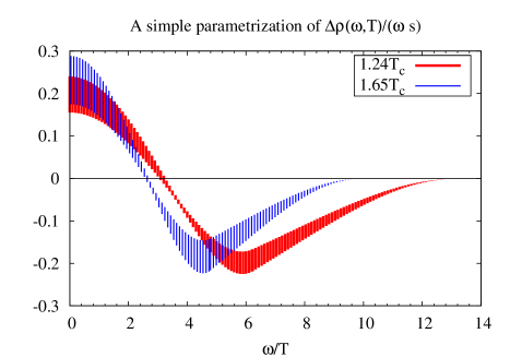
Figure 5: A smooth parametrization of the thermal part of the subtracted spectral function, $\Delta\rho_{\star}(\omega,T)/(\omega\cdot s)$, compatible with the bulk sum rule and the lattice correlator at $t=\beta/2$. Recall that the ratio $\zeta/s$ is given by $\frac{\pi}{9}\times$ the intercept of this function.

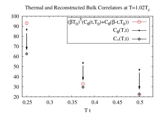
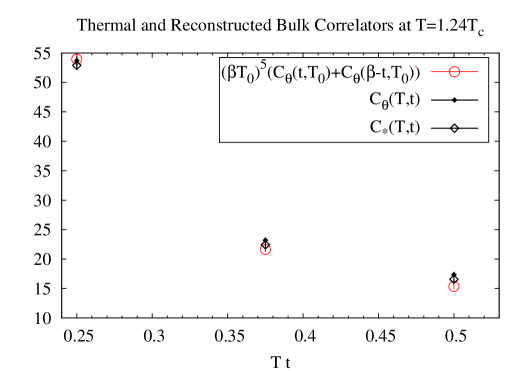
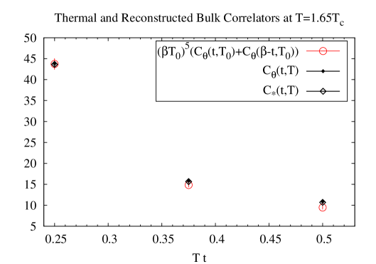
Figure 6: Bulk-channel correlators at three temperatures. Here $N_{\tau}=8$ and treelevel-improvement has been applied. The open circles correspond to what the Euclidean correlator would be if the spectral density remained unchanged from a much lower temperature, $T_{0}\simeq T_{c}/2$.

While no detailed properties of $\Delta\rho_{\star}$ can be determined based on the limited information at hand, we want to show somewhat more quantitatively how Eq. (72) and (73) dictate the rearrangement of the spectral weight. For instance, in an interval of frequencies, one may ask whether $\int_{\omega_{1}}^{\omega_{2}}\frac{d\omega}{\omega}\Delta\rho_{\star}$ is positive or negative. In order to address this question in a systematic way, we apply the following procedure (it is of course not unique). We select a binning in the frequency variable $\omega$. We choose $[0,\omega_{1}]$ and $[\omega_{1},\omega_{2}]$. The upper end of the second bin, $\omega_{2}$, is chosen large enough for the OPE to be reliable. Since $\rho_{\star}(\omega,T=0)$ vanishes for $\omega<m$, it is of physical interest to choose $\omega_{1}$ on the order of $m$.

Second, since we expect the (infinite-volume) spectral function to be smooth at least at high-frequencies, we parametrize $\Delta\rho_{\star}$ by a second-order polynomial in $\omega^{2}$ in each bin. We require continuity and differentiability at the boundaries between the bins. For $\omega>\omega_{2}$, we use the expression provided by the OPE. This then leaves 6 coefficients to be determined. Four equations are provided by the matching conditions at the edges of the bins, and two are provided by the known frequency integrals of $\Delta\rho_{\star}$, Eq. (72) and (73). Determining this simple parametrization of the spectral function thus amounts, in the present case, to inverting a $6\times 6$ matrix.

The result of this procedure is show in Fig. (5). The bands indicate the statistical error obtained by standard error propagation. These curves show qualitatively what was expected from the remarks below Eq. (73), namely the appearance of a positive spectral weight for $\omega<m$, and a depletion relative to the vacuum spectral density for $\omega>m$. Incidentally, this is qualitatively consistent with the prediction of perturbation theory, where the O($\alpha_{s}^{2}$) low-frequency and O($\alpha_{s}^{2}$) high-frequency contributions cancel eachother, resulting in a spectral sum $\int d\omega\Delta\rho_{\star}/\omega$ that is O($\alpha_{s}^{3}$) [34, 29].

We note that the values of the intercept in Fig. (5) at $1.24T_{c}$ and $1.65T_{c}$, although strongly dependent on the fact that we have smoothened the spectral function, are in good agreement with our previous estimates for $\zeta/s$ [19], where the unsubtracted spectral function $\rho_{\theta}$ was directly parametrized. This may well be because in both cases we made a smooth ansatz for the spectral function, but in view of the large cancellation that occurs in $\Delta\rho_{\star}$, the consistency is not totally trivial.

5 Conclusion

We have collected information, obtained by analytic methods, on the spectral density of the bulk channel in SU($N$) gauge theory. We have reviewed the precise connection between the Euclidean and the retarded correlator in frequency space, illustrated in Fig. (1), recalculated the OPE of the bulk channel correlator, Eq. (43), and presented a new way, based on (Eq. 25), to compute the reconstructed correlator. The latter technique allows one to directly constrain the difference of thermal to vacuum spectral densities, $\Delta\rho$.

Numerically, we have found that in the deconfined phase of SU(3) gauge theory, a significant depletion of the spectral density must take place in the interval $m\lesssim\omega\lesssim 3m$, while we have presented evidence that a non-vanishing spectral density appears at frequencies below the mass gap, obviously a finite-temperature effect. This qualitative conclusion comes from combining the bulk sum rule with numerical lattice correlators. With numerical data of higher accuracy, it would be possible to quantify more precisely how much spectral weight is clustered around the origin with frequencies $\omega\lesssim T$.

Unfortunately, the behavior of the bulk spectral function at low frequencies near the deconfining temperature remains largely undetermined. The Euclidean correlator $C(t,T\approx T_{c})$ clearly exhibits an enhancement compared to higher temperatures, even after subtraction of the $t$-independent contribution, see Eq. (54), which is quite large just above the transition. However this enhancement can be explained to a large extent by the properties of the vacuum, as the comparison with the reconstructed correlator shows. At the moment we can state that a depletion of the spectral density has to take place for frequencies above the mass gap, in view of the bulk sum rule, but are unable at present to give a useful estimate of the spectral weight below the mass gap. This more careful reanalysis of the bulk channel has taught us that the effects of a potentially large bulk viscosity near $T_{c}$ are more subtle to detect in spectral integrals than previous work suggested [17, 19]. More accurate lattice data, in particular for the speed of sound near the phase transition, would allow one to determine the cumulated spectral weight below the mass gap. We believe that this goal can be achieved in the foreseeable future.

Appendix A Spectral representation of finite-temperature correlators

In this appendix we give the spectral representation of various correlators. We use this representation to obtain Eq. (11).

A.1 Real-time correlators

Inserting two complete sets of energy eigenstates in the expression (3) for $G_{R}(t)$, one obtains

$$G_{R}(t)=\frac{i\theta(t)}{Z}\sum_{m,n}|O_{nm}|^{2}e^{-\beta E_{n}}(e^{iE_{nm}t}-e^{-iE_{nm}t})\,,$$ (80)

where we employ the notation

$$E_{nm}=E_{n}-E_{m}\,,\qquad O_{nm}=\langle n|\hat{\cal O}(t=0)|m\rangle\,.$$ (81)

In the same representation, the Fourier transform (4) reads, for $\mathop{\rm Im}\omega>0$,

$$\tilde{G}_{R}(\omega) = \frac{1}{Z}\sum_{m,n}|O_{nm}|^{2}e^{-\beta E_{n}}\left(\frac{1}{\omega-E_{nm}}-\frac{1}{\omega+E_{nm}}\right)$$ (82)

$$= \frac{1}{Z}\sum_{m,n}|O_{nm}|^{2}e^{-\beta E_{n}}\frac{2E_{nm}}{\omega^{2}-E_{nm}^{2}}\,.$$ (83)

In particular, for later reference,

$$\tilde{G}_{R}(i\omega_{\rm I}) = -\frac{1}{Z}\sum_{n,m}|O_{nm}|^{2}e^{-\beta E_{n}}\frac{2E_{nm}}{\omega_{\rm I}^{2}+E_{nm}^{2}}\,$$ (84)

$$= \frac{\beta}{Z}\sum_{n,m}|O_{nm}|^{2}e^{-\beta(E_{n}+E_{m})/2}\frac{E_{nm}^{2}}{\omega_{\rm I}^{2}+E_{nm}^{2}}\frac{\sinh(\beta E_{nm}/2)}{\beta E_{nm}/2}\quad(\omega_{\rm I}>0).$$ (85)

A.2 Euclidean correlators

The spectral representation of the Euclidean correlator (5) reads

$$G_{E}(t)=\frac{1}{Z}\sum_{n,m}|O_{nm}|^{2}e^{-\beta E_{n}}e^{E_{nm}t}\,,$$ (86)

and after some algebraic manipulations, one also finds for the Fourier coefficients (8)

$$G_{E}^{(\ell)}=\frac{\beta}{Z}\sum_{m,n}|O_{nm}|^{2}e^{-\beta(E_{n}+E_{m})/2}\frac{E_{nm}^{2}}{\omega_{\ell}^{2}+E_{nm}^{2}}\frac{\sinh(\beta E_{nm}/2)}{\beta E_{nm}/2}$$ (87)

Thus in particular we see that Eq. (9) holds.

The relation of the Matsubara zero-mode $\ell=0$ with the zero-frequency retarded correlator requires special care. Using the spectral representation, one finds

$$G_{E}^{(0)}-G_{R}(i\omega_{\rm I}) = \frac{\beta}{Z}\sum_{m,n}|O_{nm}|^{2}e^{-\beta(E_{n}+E_{m})/2}\frac{\sinh(\beta E_{nm}/2)}{\beta E_{nm}/2}\frac{\omega_{\rm I}^{2}}{\omega_{\rm I}^{2}+E_{nm}^{2}}\,.$$ (88)

In the next section, we shall see that the right-hand side can be expressed in terms of the spectral function.

A.3 The spectral function, and its relation to Euclidean correlators

Taking the imaginary part of the retarded correlator, Eq. (82), one obtains

$$\mathop{\rm Im}\tilde{G}_{R}(\omega)=\frac{1}{Z}\sum_{n,m}|O_{nm}|^{2}e^{-\beta E_{n}}\left(\frac{\omega_{\rm I}}{(\omega_{\rm R}+E_{nm})^{2}+\omega_{\rm I}^{2}}-\frac{\omega_{\rm I}}{(\omega_{\rm R}-E_{nm})^{2}+\omega_{\rm I}^{2}}\right)$$ (89)

For a complex frequency just above the real axis, $\omega_{\rm I}=\epsilon$, we obtain

$$\mathop{\rm Im}\tilde{G}_{R}(\omega+i\epsilon)=\frac{\pi}{Z}\sum_{n,m}|O_{nm}|^{2}e^{-\beta E_{n}}[\delta(\omega+E_{nm})-\delta(\omega-E_{nm})]\,,~{}~{}\omega\in{\bf R}.$$ (90)

We have used one of the standard representations of the delta function,

$$\delta(\omega)=\frac{1}{\pi}\frac{\epsilon}{\omega^{2}+\epsilon^{2}}\,.$$ (91)

Symmetrizing the sum in Eq. (90) with respect to $m$ and $n$, one easily reaches the form ($\omega\in{\bf R}$)

$$\rho(\omega)=\frac{1}{\pi}\lim_{\epsilon\to 0}{\rm Im}\tilde{G}_{R}(\omega+i\epsilon)=\frac{2}{Z}\,\sin\frac{\beta\omega}{2}\sum_{m,n}|O_{nm}|^{2}e^{-\beta(E_{n}+E_{m})/2}\delta(\omega-E_{nm})\,.$$ (92)

We thus observe that the limit of $\tilde{G}_{R}$ for $\omega$ approaching the real axis is in general a distribution.

1. It is easy to verify, using Eq. (86) and (92), that the Euclidean correlator can be obtained from $\rho$ via Eq. (12).

2. Substituting (92) into the right-hand side of Eq. (11), one recovers Eq. (88), thus proving Eq. (11).

3. A simple calculation based on expression (92) formally leads to Eq. (14).

References

- [1] BRAHMS Collaboration, I. Arsene et. al., Quark gluon plasma and color glass condensate at RHIC? The perspective from the BRAHMS experiment, Nucl. Phys. A757 (2005) 1–27, [nucl-ex/0410020].
- [2] B. B. Back et. al., The PHOBOS perspective on discoveries at RHIC, Nucl. Phys. A757 (2005) 28–101, [nucl-ex/0410022].
- [3] PHENIX Collaboration, K. Adcox et. al., Formation of dense partonic matter in relativistic nucleus nucleus collisions at RHIC: Experimental evaluation by the PHENIX collaboration, Nucl. Phys. A757 (2005) 184–283, [nucl-ex/0410003].
- [4] STAR Collaboration, J. Adams et. al., Experimental and theoretical challenges in the search for the quark gluon plasma: The STAR collaboration’s critical assessment of the evidence from RHIC collisions, Nucl. Phys. A757 (2005) 102–183, [nucl-ex/0501009].
- [5] J. I. Kapusta and C. Gale, Finite-temperature field theory: Principles and applications, . Cambridge, UK: Univ. Pr. (2006) 428 p.
- [6] C. DeTar and U. M. Heller, QCD Thermodynamics from the Lattice, Eur. Phys. J. A41 (2009) 405–437, [arXiv:0905.2949].
- [7] D. A. Teaney, Viscous Hydrodynamics and the Quark Gluon Plasma, arXiv:0905.2433.
- [8] P. Romatschke and U. Romatschke, Viscosity Information from Relativistic Nuclear Collisions: How Perfect is the Fluid Observed at RHIC?, Phys. Rev. Lett. 99 (2007) 172301, [arXiv:0706.1522].
- [9] H. Song and U. W. Heinz, Causal viscous hydrodynamics in 2+1 dimensions for relativistic heavy-ion collisions, Phys. Rev. C77 (2008) 064901, [arXiv:0712.3715].
- [10] K. Dusling and D. Teaney, Simulating elliptic flow with viscous hydrodynamics, Phys. Rev. C77 (2008) 034905, [arXiv:0710.5932].
- [11] M. Luzum and P. Romatschke, Conformal Relativistic Viscous Hydrodynamics: Applications to RHIC, arXiv:0804.4015.
- [12] U. W. Heinz, J. S. Moreland, and H. Song, Viscosity from elliptic flow: the path to precision, Phys. Rev. C80 (2009) 061901, [arXiv:0908.2617].
- [13] H. Song and U. W. Heinz, Interplay of shear and bulk viscosity in generating flow in heavy-ion collisions, arXiv:0909.1549.
- [14] K. Rajagopal and N. Tripuraneni, Bulk Viscosity and Cavitation in Boost-Invariant Hydrodynamic Expansion, arXiv:0908.1785.
- [15] P. Arnold, C. Dogan, and G. D. Moore, The bulk viscosity of high-temperature QCD, Phys. Rev. D74 (2006) 085021, [hep-ph/0608012].
- [16] J. I. Kapusta, Viscous Properties of Strongly Interacting Matter at High Temperature, arXiv:0809.3746.
- [17] D. Kharzeev and K. Tuchin, Bulk viscosity of QCD matter near the critical temperature, JHEP 09 (2008) 093, [arXiv:0705.4280].
- [18] F. Karsch, D. Kharzeev, and K. Tuchin, Universal properties of bulk viscosity near the QCD phase transition, Phys. Lett. B663 (2008) 217–221, [arXiv:0711.0914].
- [19] H. B. Meyer, A calculation of the bulk viscosity in SU(3) gluodynamics, Phys. Rev. Lett. 100 (2008) 162001, [arXiv:0710.3717].
- [20] S. S. Gubser, A. Nellore, S. S. Pufu, and F. D. Rocha, Thermodynamics and bulk viscosity of approximate black hole duals to finite temperature quantum chromodynamics, Phys. Rev. Lett. 101 (2008) 131601, [arXiv:0804.1950].
- [21] M. A. Stephanov, QCD phase diagram and the critical point, Prog. Theor. Phys. Suppl. 153 (2004) 139–156, [hep-ph/0402115].
- [22] D. T. Son and M. A. Stephanov, Dynamic universality class of the QCD critical point, Phys. Rev. D70 (2004) 056001, [hep-ph/0401052].
- [23] H. B. Meyer, Finite Temperature Sum Rules in Lattice Gauge Theory, Nucl. Phys. B795 (2008) 230–242, [arXiv:0711.0738].
- [24] S. Datta, F. Karsch, P. Petreczky, and I. Wetzorke, Behavior of charmonium systems after deconfinement, Phys. Rev. D69 (2004) 094507, [hep-lat/0312037].
- [25] D. Teaney, Finite temperature spectral densities of momentum and R- charge correlators in N = 4 Yang Mills theory, Phys. Rev. D74 (2006) 045025, [hep-ph/0602044].
- [26] H. B. Meyer, Energy-momentum tensor correlators and spectral functions, JHEP 08 (2008) 031, [arXiv:0806.3914].
- [27] V. A. Novikov, M. A. Shifman, A. I. Vainshtein, and V. I. Zakharov, In a Search for Scalar Gluonium, Nucl. Phys. B165 (1980) 67.
- [28] H. Forkel, Direct instantons, topological charge screening and QCD glueball sum rules, Phys. Rev. D71 (2005) 054008, [hep-ph/0312049].
- [29] S. Caron-Huot, Asymptotics of thermal spectral functions, Phys. Rev. D79 (2009) 125009, [arXiv:0903.3958].
- [30] V. A. Novikov, M. A. Shifman, A. I. Vainshtein, and V. I. Zakharov, Calculations in External Fields in Quantum Chromodynamics. Technical Review, Fortschr. Phys. 32 (1984) 585.
- [31] S.-z. Huang and M. Lissia, Constraining spectral functions at finite temperature and chemical potential with exact sum rules in asymptotically free theories, Phys. Rev. D52 (1995) 1134–1149, [hep-ph/9412246].
- [32] J. I. Kapusta and E. V. Shuryak, Weinberg type sum rules at zero and finite temperature, Phys. Rev. D49 (1994) 4694–4704, [hep-ph/9312245].
- [33] P. J. Ellis, J. I. Kapusta, and H.-B. Tang, Low-energy theorems for gluodynamics at finite temperature, Phys. Lett. B443 (1998) 63–68, [nucl-th/9807071].
- [34] P. Romatschke and D. T. Son, Spectral sum rules for the quark-gluon plasma, Phys. Rev. D80 (2009) 065021, [arXiv:0903.3946].
- [35] K. G. Wilson, Confinement of quarks, Phys. Rev. D10 (1974) 2445–2459.
- [36] M. Creutz, Monte Carlo Study of Quantized SU(2) Gauge Theory, Phys. Rev. D21 (1980) 2308–2315.
- [37] N. Cabibbo and E. Marinari, A New Method for Updating SU(N) Matrices in Computer Simulations of Gauge Theories, Phys. Lett. B119 (1982) 387–390.
- [38] A. D. Kennedy and B. J. Pendleton, Improved Heat Bath Method for Monte Carlo Calculations in Lattice Gauge Theories, Phys. Lett. B156 (1985) 393–399.
- [39] K. Fabricius and O. Haan, Heat Bath Method for the Twisted Eguchi-Kawai Model, Phys. Lett. B143 (1984) 459.
- [40] H. B. Meyer, Locality and statistical error reduction on correlation functions, JHEP 01 (2003) 048, [hep-lat/0209145].
- [41] H. B. Meyer, The Yang-Mills spectrum from a 2-level algorithm, JHEP 01 (2004) 030, [hep-lat/0312034].
- [42] S. Necco and R. Sommer, The N(f) = 0 heavy quark potential from short to intermediate distances, Nucl. Phys. B622 (2002) 328–346, [hep-lat/0108008].
- [43] K. Kajantie, M. Laine, K. Rummukainen, and Y. Schroeder, The pressure of hot QCD up to g**6 ln(1/g), Phys. Rev. D67 (2003) 105008, [hep-ph/0211321].
- [44] H. B. Meyer, Cutoff Effects on Energy-Momentum Tensor Correlators in Lattice Gauge Theory, JHEP 06 (2009) 077, [arXiv:0904.1806].
- [45] H. B. Meyer, High-Precision Thermodynamics and Hagedorn Density of States, Phys. Rev. D80 (2009) 051502, [arXiv:0905.4229].
- [46] M. Luscher, R. Sommer, P. Weisz, and U. Wolff, A Precise determination of the running coupling in the SU(3) Yang-Mills theory, Nucl. Phys. B413 (1994) 481–502, [hep-lat/9309005].
- [47] H. B. Meyer, Computing the viscosity of the QGP on the lattice, Prog. Theor. Phys. Suppl. 174 (2008) 220–227, [arXiv:0805.4567].
- [48] H. B. Meyer, Glueball matrix elements: a lattice calculation and applications, JHEP 01 (2009) 071, [arXiv:0808.3151].