On the Zero-Dispersion Limit of the Benjamin-Ono Cauchy Problem for Positive Initial Data

Abstract.

We study the Cauchy initial-value problem for the Benjamin-Ono equation in the zero-disperion limit, and we establish the existence of this limit in a certain weak sense by developing an appropriate analogue of the method invented by Lax and Levermore to analyze the corresponding limit for the Korteweg-de Vries equation.

1. Introduction

The Benjamin-Ono (BO) equation

(1) $$\frac{\partial u_{\epsilon}}{\partial t}+2u_{\epsilon}\frac{\partial u_{\epsilon}}{\partial x}+\epsilon\mathcal{H}\left[\frac{\partial^{2}u_{\epsilon}}{\partial x^{2}}\right]=0,\quad x\in\mathbb{R},\quad t>0,$$

where $\epsilon>0$ is a constant and $\mathcal{H}$ is the Hilbert transform operator defined by the Cauchy principal value integral

(2) $$\mathcal{H}[f](x):=\frac{1}{\pi}\mathchoice{{\vbox{\hbox{$\textstyle-$}}\kern-4.86108pt}}{{\vbox{\hbox{$\scriptstyle-$}}\kern-3.25pt}}{{\vbox{\hbox{$\scriptscriptstyle-$}}\kern-2.29166pt}}{{\vbox{\hbox{$\scriptscriptstyle-$}}\kern-1.875pt}}\!\int_{\mathbb{R}}\frac{f(y)}{y-x}\,dy$$

is a model for weakly nonlinear dispersive waves on the interface between two ideal immiscible fluids, one of which may be considered to be infinitely deep. Applications include the modeling of internal waves in deep water [2, 7, 29, 4], and also the modeling of atmospheric waves like the dramatic “morning glory” phenomenon of northeastern Australia [28]. The relevant Cauchy problem is to determine the solution $u_{\epsilon}(x,t)$ of (1) subject to a suitable initial condition $u_{\epsilon}(x,0)=u_{0}(x)$ given for all $x\in\mathbb{R}$.

The parameter $\epsilon>0$ is a measure of the relative strength of the dispersive and nonlinear effects in the system. In many applications one thinks of $\epsilon$ as a small parameter in part because numerical experiments show that in this situation the finite-time formation of a shock wave (gradient catastrophe) in the formal limiting equation (obtained simply by setting $\epsilon=0$ in (1)) is dispersively regularized by the generation of a smoothly modulated train of approximately periodic traveling waves, which correspond to so-called undular bores frequently observed in the evolution of physical internal waves. Snapshots from the solution of a Cauchy problem for (1) illustrating the averted shock and onset of an undular bore are shown in Figure 1.

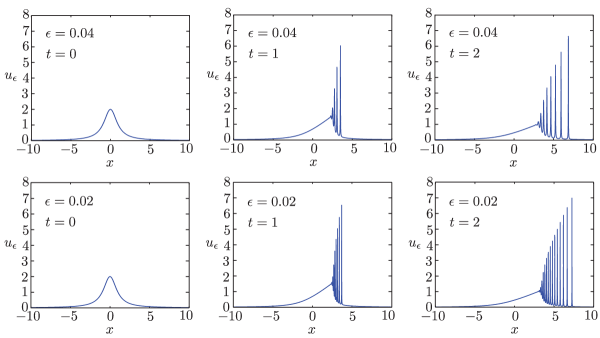
Figure 1. The evolution of a pulse under the BO equation. Top row: $\epsilon=0.04$. Bottom row: $\epsilon=0.02$. In both cases the initial condition is the same: $u_{0}(x)=2(1+x^{2})^{-1}$.

These figures clearly show that the mathematical description of the undular bore consists of waves of amplitude independent of $\epsilon$ and wavelength approximately proportional to $\epsilon$. We refer to the asymptotic analysis of the solution of the Cauchy problem with $\epsilon$-independent initial data $u_{0}(x)$ in the limit $\epsilon\downarrow 0$ as the zero-dispersion limit.

1.1. A related problem and its history

A more famous nonlinear dispersive wave equation is the Korteweg-de Vries (KdV) equation

(3) $$\frac{\partial v_{\epsilon}}{\partial t}+2v_{\epsilon}\frac{\partial v_{\epsilon}}{\partial x}+\frac{1}{3}\epsilon^{2}\frac{\partial^{3}v_{\epsilon}}{\partial x^{3}}=0,\quad x\in\mathbb{R},\quad t>0,$$

a model for long surface waves on shallow water among a wide variety of other physical phenomena. When $\epsilon>0$ is small, this equation displays qualitatively similar behavior to that just illustrated for the BO equation: the dispersive term arrests the shock in the $\epsilon=0$ equation with the formation of a train of waves of amplitude approximately independent of $\epsilon$ and wavelength proportional to $\epsilon$.

The modeling of the zero-dispersion limit for the KdV equation has a long history going back to the work of Whitham [31] who used the method of averaging to propose a nonlinear hyperbolic system of three partial differential equations to describe the modulational variables (e.g. slowly-varying amplitude, mean, and wavelength of the wavetrain). Whitham noted that the system of modulation equations he obtained had the nongeneric property that by choice of special dependent variables $v^{1}$, $v^{2}$, and $v^{3}$, it could be written in so-called Riemann invariant form, in which the three equations are only coupled through the characteristic velocities:

(4) $$\frac{\partial v^{i}}{\partial t}+c^{i}(v^{1},v^{2},v^{3})\frac{\partial v^{i}}{\partial x}=0,\quad i=1,2,3.$$

Later, Gurevich and Pitaevskii [14] considered the problem of patching together solutions of Whitham’s modulational system with solutions of the formal limiting equation (obtained by setting $\epsilon=0$ in (3)) at two moving boundary points that delineate the oscillation zone; their goal was to provide a reasonable global approximation scheme for the solution of the initial-value problem for the KdV equation (3) in the zero-dispersion limit subject to given initial data $v_{\epsilon}(x,0)=v_{0}(x)$ independent of $\epsilon$.

In the meantime, it was of course discovered that the KdV equation is a completely integrable system, posessing a compatible structure now called a Lax pair and a coincident solution procedure for addressing the Cauchy (initial-value) problem: the inverse-scattering transform. This development suggested that the methodology invented by Whitham could perhaps be placed on completely rigorous mathematical footing. After the exact periodic (and quasiperiodic) solutions of the KdV equation (3) were given a spectral interpretation by Its and Matveev [15] and Dubrovin, Matveev, and Novikov [11], the Whitham modulation equations themselves were reinterpreted within the framework of integrability by Flaschka, Forest, and McLaughlin [12]. (In particular this work made clear the reason why Whitham’s equations could be placed in Riemann invariant form; it is a consequence of integrability.)

The task that remained in the use of integrable machinery to study the zero-dispersion limit of the KdV equation was to rigorously analyze the Cauchy problem using the inverse-scattering transform. The first step in this program was taken by Lax and Levermore [20] who considered positive initial data $v_{0}(x)$ rapidly decaying to zero for large $|x|$. They used WKB methods to argue that the Schrödinger operator with potential $-v_{0}(x)$ that arises in the scattering theory is approximately reflectionless in the limit $\epsilon\downarrow 0$. On an ad-hoc basis they replaced the true scattering data by its WKB analogue, retaining only contributions from a set of $N(\epsilon)\sim\epsilon^{-1}$ discrete eigenvalues which are approximated by a Bohr-Sommerfeld quantization rule, which amounts to replacing the solution $v_{\epsilon}(x,t)$ of the Cauchy problem with another solution $\tilde{v}_{\epsilon}(x,t)$ of (3) having $\epsilon$-dependent initial data close to $v_{0}$. In this situation, the inverse-scattering procedure reduces to finite-dimensional (of dimension $N(\epsilon)$) linear algebra, and in fact the solution obtained by Cramer’s rule can be reduced to the determinantal formula

(5) $$\tilde{v}_{\epsilon}(x,t)=2\epsilon^{2}\frac{\partial^{2}}{\partial x^{2}}\log(\tau(x,t)),\quad\tau(x,t)=\det(\mathbb{I}+\mathbf{G}(x,t)),$$

where $\mathbf{G}(x,t)$ is a positive-definite real symmetric matrix of dimension $N(\epsilon)\times N(\epsilon)$. Lax and Levermore then established the existence of the limit of $2\epsilon^{2}\log(\tau(x,t))$ as $\epsilon\downarrow 0$, uniformly on compact subsets of the $(x,t)$-plane. This yields weak convergence of $\tilde{v}_{\epsilon}(x,t)$ by differentiation of the limit function with respect to $x$. The Lax-Levermore method is to expand the determinant $\tau(x,t)$ in principal minors indexed by subsets of the set of eigenvalues; noting that each term is positive they showed that the sum of terms is asymptotically dominated by its largest term, and they further approximated this discrete optimization problem with an $\epsilon$-independent (limiting) convex variational problem, explicitly parametrized by $x$ and $t$, for measures. The weak zero-dispersion limit of the Cauchy problem for the KdV equation is therefore encoded implicitly in the solution of this variational problem. The Lax-Levermore method reproduces the specified initial data $v_{0}(x)$ at $t=0$ as $\epsilon\downarrow 0$, which establishes validity, in a certain sense, of the WKB-based spectral approximation procedure in the first step.

Later, Venakides [30] was able to extend the method of Lax and Levermore to higher order, capturing the form of the oscillations that are averaged out in the weak limit. This work at last made clear that the solution of the Cauchy problem for the KdV equation with smooth, $\epsilon$-independent initial data $v_{0}(x)$ really does generate after some fixed breaking time a train of high-frequency waves of exactly the kind originally considered without complete justification by Whitham. More recently, the powerful steepest-descent method for matrix Riemann-Hilbert problems developed by Deift and Zhou was used to analyze the zero-dispersion limit for the KdV equation [8]. This technique is best viewed as a tool for converting weak asymptotics (the solution of the Lax-Levermore variational problem) into strong asymptotics (an improvement of the Venakides asymptotics in which the phase of the waveform is accurate to very high order).

1.2. The zero-dispersion limit of the Benjamin-Ono equation

It turns out that the BO equation (1) is also an integrable equation, in the sense that it has a representation as the compatibility condition of an overdetermined Lax pair of linear problems [3]. In fact, both BO and KdV equations may be viewed as limiting cases (as depth of a fluid layer tends to infinity and zero, respectively) of the so-called intermediate long-wave equation [18], itself an integrable system for arbitrary layer depth. However, the integrable structure of the BO equation is markedly different from that of the KdV equation. In particular, the nonlocality in the equation due to the presence of the Hilbert transform is mirrored in a certain nonlocality of the scattering and inverse-scattering problems. In place of the spectral theory of the selfadjoint Schrödinger (Sturm-Liouville) differential operator one has to work with the spectral theory of the nonlocal operator

(6) $$\mathcal{L}:=-i\epsilon\frac{\partial}{\partial x}-\mathcal{C}_{+}\circ u_{\epsilon}\circ\mathcal{C}_{+},\quad\mathcal{C}_{+}[f](x):=\lim_{\delta\downarrow 0}\frac{1}{2\pi i}\int_{\mathbb{R}}\frac{f(y)}{y-x-i\delta}\,dy.$$

Here, the operator $\mathcal{C}_{+}$ is the selfadjoint orthogonal projection from $L^{2}(\mathbb{R})$ onto the Hardy space of the upper half-plane, the Hilbert space on which $\mathcal{L}$ is selfadjoint, and $u_{\epsilon}$ denotes the operator of multiplication by $u_{\epsilon}(\cdot,t)$.

Certainly a key step forward in the theory of the zero-dispersion limit was taken by Dobrokhotov and Krichever [9] who noted that the second (time evolution) equation in the Lax pair for the BO equation (see (30) below) is simply a time-dependent Schrödinger equation whose potential is a function with an analytic continuation from the real $x$-axis into the upper half-plane and were able to adapt a pre-existing construction of “integrable” potentials for this equation to the appropriate Hardy-space setting. This allowed them to construct, from the Lax pair, a large family of periodic traveling wave solutions of the BO equation (1), along with quasiperiodic generalizations. Remarkably, unlike the corresponding exact solutions of the KdV equation (3) which are highly transcendental objects constructed from Riemann theta functions of hyperelliptic curves of arbitrary genus, the periodic and quasiperiodic solutions of the BO equation turn out to be simple rational functions of $P$ exponential phases $e^{i(k_{j}x-\omega_{j}t)/\epsilon}$. In the same paper, Dobrokhotov and Krichever also carried out for the BO equation the analogue of the calculation of Flaschka, Forest, and McLaughlin [12], deriving by multiphase averaging a system of equations governing the modulational variables for a slowly-varying train of $P$-phase waves. Here we arrive at a second remarkable fact: not only can the modulation equations be written in Riemann invariant form, they are completely diagonal:

(7) $$\frac{\partial u^{i}}{\partial t}+2u^{i}\frac{\partial u^{i}}{\partial x}=0,\quad i=1,\dots,2P+1$$

(the case of $P=1$ corresponds to simple traveling waves). This again should be contrasted with the situation for the KdV equation in which the characteristic velocities not only provide coupling among the fields but also are transcendental functions of the fields written in terms of ratios of complete hyperelliptic integrals.

The analogue for the BO equation of the matching procedure developed by Gurevich and Pitaevskii [14] to describe the evolution of a dispersive shock was independently described by Matsuno [24, 25] and by Jorge, Minzoni, and Smyth [16]. This matching procedure provides a reasonable approach to the Cauchy problem for the Benjamin-Ono equation (1) with fixed initial data $u_{\epsilon}(x,0)=u_{0}(x)$ when $\epsilon\ll 1$, but it is based on formal asymptotics. In [24], Matsuno writes:

From a rigorously mathematical point of view, however, the various results presented in this paper should be justified on the basis of an exact method of solution such as [the inverse-scattering transform], or an analog of the Lax-Levermore theory for the KdV equation.

It is our intention in this paper to provide exactly such a justification, by developing a new method that does for the BO Cauchy problem exactly what the Lax-Levermore method does for the KdV Cauchy problem.

The main result of our analysis is remarkably easy to state, but first we need to recall some basic facts concerning the equation obtained from (1) simply by setting $\epsilon=0$. Recall that while for general sufficiently smooth initial data $u^{\mathrm{B}}(x,0)=u_{0}(x)$ the inviscid Burgers equation

(8) $$\frac{\partial u^{\mathrm{B}}}{\partial t}+2u^{\mathrm{B}}\frac{\partial u^{\mathrm{B}}}{\partial x}=0$$

does not have a global solution as a function due to gradient catastrophe (shock formation) in finite time, it does have a global solution as a real multi-sheeted surface over the $(x,t)$-plane; indeed this is the construction of the method of characteristics. The sheets of this surface are obtained as the real solutions of the implicit equation

(9) $$u^{\mathrm{B}}=u_{0}(x-2u^{\mathrm{B}}t),$$

and by implicit differentiation it is easy to verify that away from singularities each sheet of the surface is a function $u^{\mathrm{B}}=u^{\mathrm{B}}(x,t)$ that satisfies (8). A simple consequence of the Implicit Function Theorem is that for sufficiently small $|t|$ there is a unique solution of (9) for all $x\in\mathbb{R}$. New sheets of the multivalued solution are born from breaking points in the $(x,t)$-plane that are in one-to-one correspondence with generic inflection points $\xi$ of $u_{0}$ for which $u_{0}^{\prime}(\xi)\neq 0$ but $u_{0}^{\prime\prime}(\xi)=0$. If $\xi\in\mathbb{R}$ is such a point, then the corresponding breaking point is given by

(10) $$(x_{\xi},t_{\xi}):=\left(\xi-\frac{u_{0}(\xi)}{u_{0}^{\prime}(\xi)},-\frac{1}{2u_{0}^{\prime}(\xi)}\right).$$

Each such breaking point is the location of a pitchfork bifurcation for $u^{\mathrm{B}}$ with respect to $t$ holding $x-2u_{0}(\xi)t=\xi$ fixed, with two new branches emerging as $|t|$ increases. Thus, assuming that $u_{0}^{\prime}$ is a bounded function of total integral zero, the solution of the Cauchy problem for (8) is classical for

(11) $$T_{-}:=-\frac{1}{2\max_{x\in\mathbb{R}}u_{0}^{\prime}(x)}<t<-\frac{1}{2\min_{x\in\mathbb{R}}u_{0}^{\prime}(x)}=:T_{+}.$$

Note that under our assumptions on $u_{0}^{\prime}$ we have $T_{-}<0<T_{+}$. Also, $T_{-}$ is the supremum of all $t_{\xi}<0$ while $T_{+}$ is the infimum of all $t_{\xi}>0$. When we consider the Cauchy problem for $t>0$, we will refer to $T:=T_{+}$ as the breaking time.

For $t/t_{\xi}>1$ there are caustic curves $x^{-}_{\xi}(t)<x^{+}_{\xi}(t)$ with limiting values as $t\to t_{\xi}$ given by $x^{-}_{\xi}(t_{\xi})=x^{+}_{\xi}(t_{\xi})=x_{\xi}$ that bound the triply-folded region emerging from $(x_{\xi},t_{\xi})$. The caustic curves correspond to double roots of (9), and crossing one of them at a generic point results in a change in the number of sheets by exactly two. Except along the union of the caustic curves and the breaking points from which they emerge, the number of solutions of (9) is always odd, and all are simple roots. See Figure 2.

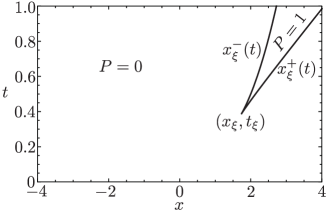
Figure 2. Except along the caustic curves $x=x^{-}_{\xi}(t)$ and $x=x^{+}_{\xi}(t)$ the number of solutions of (9) is of the form $2P+1$, and these solutions are simple roots. For this figure, $u_{0}(x):=2(1+x^{2})^{-1}$.

For the initial data $u_{0}(x)=2(1+x^{2})^{-1}$ used in Figure 1, the breaking time before which there is a unique solution for all $x\in\mathbb{R}$ and after which there is an expanding interval in which there are three solutions, is exactly $T=2\sqrt{3}/9\approx 0.3849$. Snapshots of the evolution of the multivalued solution of (8) for this initial data are shown in Figure 3.

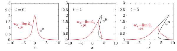
Figure 3. The multivalued solution (black) of (8) and the signed sum of branches (red) corresponding to $u_{0}(x)=2(1+x^{2})^{-1}$. Left: $t=0$. Middle: $t=1$. Right: $t=2$. Before the breaking time as well as afterwards but outside the oscillation interval there is only one solution branch and hence no difference between the red and black curves.

Our result is then the following.

Theorem 1.1.

Let $u^{\mathrm{B}}_{0}(x,t)<u^{\mathrm{B}}_{1}(x,t)<\cdots<u^{\mathrm{B}}_{2P(x,t)}(x,t)$ be the branches of the multivalued (method of characteristics) solution of the inviscid Burgers equation (8) subject to an admissible initial condition $u^{\mathrm{B}}(x,0)=u_{0}(x)$. Then, the weak $L^{2}(\mathbb{R})$ (in $x$) limit of $\tilde{u}_{\epsilon}(x,t)$ is given by

(12) $$\mathop{\mathrm{w}_{x}\mathrm{-lim}}_{\epsilon\downarrow 0}\tilde{u}_{\epsilon}(x,t)=\sum_{n=0}^{2P(x,t)}(-1)^{n}u^{\mathrm{B}}_{n}(x,t),$$

uniformly for $t$ in arbitrary bounded intervals. Note that the right-hand side extends by continuity to the caustic curves.

The signed sum of branches that is the weak limit is illustrated with red curves in Figure 3 for the same initial data as in Figure 1. Of course convergence in the weak $L^{2}(\mathbb{R})$ (in $x$) topology means that for every $v\in L^{2}(\mathbb{R})$, we have

(13) $$\lim_{\epsilon\downarrow 0}\int_{\mathbb{R}}\tilde{u}_{\epsilon}(x,t)v(x)\,dx=\int_{\mathbb{R}}\left[\sum_{n=0}^{2P(x,t)}(-1)^{n}u^{\mathrm{B}}_{n}(x,t)\right]v(x)\,dx$$

with the limit being uniform with respect to $t$ in arbitrary bounded intervals. Thus, the weak limit essentially smooths out the rapid oscillations seen in Figure 1 and (if we think of $v$ as the indicator function of a mesoscale interval) represents a kind of local average in $x$. What it means for an initial condition to be admissible will be explained later (see Definition 3.1). Here $\tilde{u}_{\epsilon}(x,t)$ is not exactly the solution of the Cauchy problem for the BO equation (1) with fixed initial data $u_{0}(x)$, but it is for every $\epsilon>0$ an exact solution of (1) that satisfies an $\epsilon$-dependent initial condition that converges (in the strong $L^{2}$ sense, see Corollary 1.1 below) to $u_{0}(\cdot)$ as $\epsilon\downarrow 0$. See Definition 3.2 for more details. This modification of the initial data is an analogue of the replacement of the true scattering data by its reflectionless WKB approximation in the Lax-Levermore theory.

For $t$ before the breaking time $T$ for Burgers’ equation, the weak limit guaranteed by Theorem 1.1 may be strengthened as follows.

Corollary 1.1.

Suppose that $0\leq t<T$, so that $P(x,t)=0$ for all $x\in\mathbb{R}$ (that is, the solution $u^{\mathrm{B}}=u^{\mathrm{B}}_{0}(x,t)$ of Burgers’ equation with initial data $u_{0}(x)$ is classical). Then

(14) $$\lim_{\epsilon\downarrow 0}\tilde{u}_{\epsilon}(x,t)=u^{\mathrm{B}}_{0}(x,t)$$

with the limit being in the (strong) $L^{2}(\mathbb{R}_{x})$ topology.

It should be pointed out that the weak limit formula (12) is much more explicit than the corresponding formula found by Lax and Levermore [20] for the weak zero-dispersion limit of the Cauchy problem for the KdV equation. Indeed, the latter requires the solution, for each $x$ and $t$, of a constrained functional variational problem, which can be solved in closed form only for the simplest initial data. As we will now see, there are several classical wave propagation problems whose asymptotic behavior can be reduced to the multivalued solution of Burgers’ equation; however, even these simple problems involve more complicated schemes for combining the solution branches than that exhibited in the simple formula (12).

After we introduce the necessary framework for our study (the inverse-scattering transform for the BO equation) in §2, we will analyze the direct scattering map in the zero-dispersion limit in §3. Then we will prove Theorem 1.1 in §4 by carrying out a detailed analysis of the inverse scattering map applied to the asymptotic formulae for scattering data obtained in §3. In §5 we prove Corollary 1.1, and then in §6 we will illustrate our results with numerical calculations and address the relation between $\tilde{u}_{\epsilon}(x,t)$ and the true solution $u_{\epsilon}(x,t)$ of the Cauchy problem for the BO equation with initial data $u_{0}$. Some comments about our continuing work can be found in the conclusion, §7. But before we embark on our study of the BO equation, we pause to consider some familiar analogues of Theorem 1.1.

1.3. Elementary examples

The key role played in the zero-dispersion limit of the BO Cauchy problem by the multivalued solution of the equation (8) with the same initial data is reminiscent of two basic example problems from the theory of linear and nonlinear waves.

1.3.1. The zero-viscosity limit of the viscous Burgers equation

The Burgers equation with viscosity $\epsilon>0$ is the nonlinear wave equation

(15) $$\frac{\partial w_{\epsilon}}{\partial t}+2w_{\epsilon}\frac{\partial w_{\epsilon}}{\partial x}-\epsilon\frac{\partial^{2}w_{\epsilon}}{\partial x^{2}}=0,\quad x\in\mathbb{R},\quad t>0$$

and we take fixed initial data $w_{\epsilon}(x,0)=u_{0}(x)$. As is well-known, this Cauchy problem is solved by the Cole-Hopf transformation, leading to the exact solution formula

(16) $$w_{\epsilon}(x,t)=\frac{1}{2t}\frac{\displaystyle\int_{\mathbb{R}}e^{R(\xi;x,t)/\epsilon}(x-\xi)\,d\xi}{\displaystyle\int_{\mathbb{R}}e^{R(\xi;x,t)/\epsilon}\,d\xi},\quad t>0,$$

where the exponent function is defined as

(17) $$R(\xi;x,t):=-\int_{0}^{\xi}u_{0}(\eta)\,d\eta-\frac{(x-\xi)^{2}}{4t}.$$

One examines the asymptotic behavior in the limit $\epsilon\downarrow 0$ by using Laplace’s method to analyze the integrals (see [26], §3.6). The dominant contributions to the integrals come from neighborhoods of points $\xi=\xi(x,t)\in\mathbb{R}$ at which $R(\xi;x,t)$ achieves its maximum value. The critical points of $R$ satisfy $\xi=x-2u_{0}(\xi)t$. Writing $u^{\mathrm{B}}=u_{0}(\xi)$ and applying $u_{0}$ to both sides gives the equation (9), so the critical points correspond to the sheets of the multivalued solution of the (inviscid) Burgers equation (8) with initial data $u_{0}$. It is easy to check that if $x$ and $t$ are such that there is just one sheet, then the unique critical point is the global maximizer of $R$ and Laplace’s method gives the result that $w_{\epsilon}(x,t)$ converges (strongly, pointwise in $x$ and $t$) to $u^{\mathrm{B}}(x,t)$. On the other hand, if there are $2P+1>1$ sheets, then for generic $(x,t)$ exactly one of them corresponds to the global maximum of $R$, and Laplace’s method predicts that $w_{\epsilon}(x,t)$ will converge to the maximizing sheet. Shocks appear in the small viscosity limit as curves in the $(x,t)$-plane along which there are jump discontinuities of the pointwise limit corresponding to sudden changes in the choice of sheet that maximizes the exponent $R$. To summarize, we have the formula

(18) $$\lim_{\epsilon\downarrow 0}w_{\epsilon}(x,t)=u^{\mathrm{B}}_{n}(x,t),\quad n=\mathop{\mathrm{argmax}}_{m=0,\dots,2P(x,t)+1}R(x-2u^{\mathrm{B}}_{m}(x,t)t;x,t)$$

for $(x,t)$ not on a shock.

Thus, one sees that for the zero-viscosity limit of the viscous Burgers equation, different sheets of the multivalued solution of the formal limiting Cauchy problem (set $\epsilon=0$) provide the strong limit of $w_{\epsilon}(x,t)$ for different $x$ and $t$. However, the choice of sheet requires the solution of a discrete maximization problem parametrized by $x$ and $t$, making the limiting behavior harder to calculate than the weak zero-dispersion limit of the BO equation.

1.3.2. The semiclassical limit of the free linear Schrödinger equation

In this problem, one considers the equation

(19) $$i\epsilon\frac{\partial\psi_{\epsilon}}{\partial t}+2\epsilon^{2}\frac{\partial^{2}\psi_{\epsilon}}{\partial x^{2}}=0,\quad x\in\mathbb{R},\quad t>0$$

for small $\epsilon>0$, subject to initial data of WKB form

(20) $$\psi_{\epsilon}(x,0)=A(x)e^{iS(x)/\epsilon}$$

with $A$ and $S$ real-valued and independent of $\epsilon$. For suitable $A$ and $S$, the solution to this problem can be written as an integral

(21) $$\psi_{\epsilon}(x,t)=\frac{e^{-i\pi/4}}{\sqrt{8\pi\epsilon t}}\int_{\mathbb{R}}e^{iI(\xi;x,t)/\epsilon}A(\xi)\,d\xi,\quad t>0,\quad I(\xi;x,t):=S(\xi)+\frac{(x-\xi)^{2}}{8t}.$$

The dominant contributions to the solution are calculated via the method of stationary phase (see [26], §5.6), and these come from small neighborhoods of points $\xi$ satisfying $I^{\prime}(\xi;x,t)=0$, that is, solutions $\xi$ of the implicit equation $\xi=x-4S^{\prime}(\xi)t$. Evaluating the function $2S^{\prime}(\cdot)$ on both sides of this equation and making the substitution $u^{\mathrm{B}}=2S^{\prime}(\xi)$, one arrives at the equivalent form (9) where $u_{0}(x):=2S^{\prime}(x)$. Thus, the branches of the multivalued solution of Burgers’ equation (8) with initial condition $u_{0}$ correspond to stationary phase points $\xi$ that yield the leading term of the solution $\psi_{\epsilon}(x,t)$ in the semiclassical limit $\epsilon\downarrow 0$. Unlike in the analysis of Laplace-type integrals, where only the critical points corresponding to maxima matter in the limit, for oscillatory integrals all stationary phase points contribute to the leading-order behavior, and therefore we have an asymptotic representation of $\psi_{\epsilon}(x,t)$ as a sum over branches $u^{\mathrm{B}}_{n}(x,t)$ of the multivalued solution of Burgers’ equation with initial data $u_{0}$:

(22) $$\psi_{\epsilon}(x,t)=\sum_{n=0}^{2P(x,t)}M_{n}(x,t)e^{i\theta_{k}(x,t;\epsilon)}+O(\epsilon),\quad t>0,$$

where $M_{n}(x,t)$ are slowly-varying positive amplitudes given by

(23) $$M_{n}(x,t):=A(x-2u_{n}^{\mathrm{B}}(x,t)t)\sqrt{\left|1-2t\frac{\partial u_{n}^{\mathrm{B}}}{\partial x}(x,t)\right|},$$

and $\theta_{k}(x,t;\epsilon)$ are rapidly-varying real phases given by

(24) $$\theta_{n}(x,t;\epsilon):=\frac{1}{\epsilon}I(x-2u_{n}^{\mathrm{B}}(x,t)t;x,t)+\frac{\pi}{4}\left(\mathrm{sgn}\left(1-2t\frac{\partial u_{n}^{\mathrm{B}}}{\partial x}(x,t)\right)-1\right),$$

for $n=0,\dots,2P(x,t)$.

A more explicit connection with the multivalued solution of Burgers’ equation may be obtained by introducing the quantity

(25) $$w_{\epsilon}(x,t):=2\epsilon\frac{\partial}{\partial x}\Im\{\log(\psi_{\epsilon}(x,t))\}$$

which is the fluid velocity in Madelung’s interpretation of the wave function $\psi_{\epsilon}$ as describing a quantum-corrected fluid motion. Under the condition that the error term in (22) becomes $O(1)$ after differentiation with respect to $x$, some easy calculations show that (22) implies

(26) $$w_{\epsilon}(x,t)=\Re\left\{\frac{\displaystyle\sum_{n=0}^{2P(x,t)}u_{n}^{B}(x,t)M_{n}(x,t)e^{i\theta_{n}(x,t;\epsilon)}}{\displaystyle\sum_{n=0}^{2P(x,t)}M_{n}(x,t)e^{i\theta_{n}(x,t;\epsilon)}}\right\}+O(\epsilon).$$

It is then easy to see that if $P(x,t)=0$, $w_{\epsilon}(x,t)$ converges strongly pointwise to $u_{0}^{B}(x,t)$, the unique solution (for this $x$ and $t$, anyway) of Burgers’ equation. On the other hand, if $P(x,t)>0$, then there are interference effects among the terms in the sums and these lead to rapid oscillations with the effect that $w_{\epsilon}(x,t)$ no longer converges in the pointwise sense as $\epsilon\downarrow 0$. However, it does converge in the weak topology. The weak limit may be computed by multiphase averaging, which we illustrate in the case $P(x,t)=1$. The procedure is to average the leading term in $w_{\epsilon}(x,t)$ over an interval in $x$ centered at the point of interest of radius, say, $\epsilon^{p}$ for some $p\in(0,1)$, and then pass to the limit $\epsilon\downarrow 0$. This produces the desired local average over rapid oscillations of wavelength or period proportional to $\epsilon$. Under an ergodic hypothesis that is valid on a set of full measure in the $(x,t)$-plane, this procedure is equivalent to holding $u^{\mathrm{B}}_{n}$ and $M_{n}$ fixed and averaging (with uniform measure) over the torus of relative angles $\phi_{1}:=\theta_{1}-\theta_{0}$ and $\phi_{2}:=\theta_{2}-\theta_{0}$. The double integrals can be evaluated explicitly, with the result that

(27) $$\mathop{\mathrm{w}_{x}\mathrm{-lim}}_{\epsilon\downarrow 0}w_{\epsilon}(x,t)=\sum_{n=0}^{2}c_{n}(x,t)u_{n}^{\mathrm{B}}(x,t),$$

where $c_{n}(x,t)$, $n=0,1,2$, are nonnegative coefficients with the property that $c_{0}(x,t)+c_{1}(x,t)+c_{2}(x,t)=1$. Specifically, the coefficients only depend on $x$ and $t$ through $M_{0}(x,t)$, $M_{1}(x,t)$, and $M_{2}(x,t)$. If any of these, say $M_{n}$, exceeds the sum of the other two, then $c_{n}=1$ and the two other coefficients vanish. Thus the weak limit produces in this case exactly the branch $u_{n}^{B}(x,t)$ through multiphase averaging. On the other hand, if none of the $M_{n}$ exceeds the sum of the other two, then $M_{0}$, $M_{1}$, and $M_{2}$ are the side lengths of a triangle, and the weak limit is a genuine weighted average of the three branches, with weights proportional to the opposite angles:

(28) $$\begin{split}c_{0}&=\frac{1}{\pi}\arccos\left(\frac{M_{1}^{2}+M_{2}^{2}-M_{0}^{2}}{2M_{1}M_{2}}\right)\\ c_{1}&=\frac{1}{\pi}\arccos\left(\frac{M_{0}^{2}+M_{2}^{2}-M_{1}^{2}}{2M_{0}M_{2}}\right)\\ c_{2}&=\frac{1}{\pi}\arccos\left(\frac{M_{0}^{2}+M_{1}^{2}-M_{2}^{2}}{2M_{0}M_{1}}\right).\end{split}$$

The most significant aspect of this analysis is that the weak limit depends on information other than just the initial condition $u_{0}$ for Burgers’ equation since the functions $M_{n}(x,t)$ involve also the initial wave function amplitude $A$. This makes the evaluation of the weak limit a more complicated procedure than in the case of the BO equation.

A further connection between the BO equation (1) and the linear Schrödinger equation (19) in the zero-dispersion limit will be made in §2.4.

2. Relevant Aspects of the Inverse Scattering Transform for the BO Cauchy Problem

2.1. The Lax pair for the BO equation and its basic properties

The Lax pair [3], whose compatibility condition is the BO equation (1), consists of the two equations

(29) $$i\epsilon\frac{\partial w^{+}}{\partial x}+\lambda(w^{+}-w^{-})=-u_{\epsilon}w^{+}$$

(30) $$i\epsilon\frac{\partial w^{\pm}}{\partial t}-2i\lambda\epsilon\frac{\partial w^{\pm}}{\partial x}+\epsilon^{2}\frac{\partial^{2}w^{\pm}}{\partial x^{2}}-2i\mathcal{C}_{\pm}\left[\epsilon\frac{\partial u_{\epsilon}}{\partial x}\right]w^{\pm}=0,$$

where $\lambda\in\mathbb{C}$ is a spectral parameter, $u_{\epsilon}=u_{\epsilon}(x,t)$ is a solution of (1), and $w^{\pm}=w^{\pm}(x,t;\lambda)$ are functions that are required to be, for each fixed $t$ and $\lambda$, the boundary values on the real $x$-axis of functions analytic in the upper ($+$) and lower ($-$) half complex $x$-plane. Also, $\pm\mathcal{C}_{\pm}=\tfrac{1}{2}\mathbb{I}\mp\tfrac{1}{2}i\mathcal{H}$ are the orthogonal and complementary ($\mathcal{C}_{+}-\mathcal{C}_{-}=\mathbb{I}$, the Plemelj formula) projections from $L^{2}(\mathbb{R})$ onto its upper and lower Hardy subspaces $\mathbb{H}^{\pm}(\mathbb{R})$. From the point of view of the inverse-scattering transform, i.e. using the Lax pair as a tool to solve the Cauchy problem, equation (29) may be considered for fixed time $t$ and defines the scattering data associated with $u_{\epsilon}(x,t)$ at time $t$. The function $w^{-}$ may be viewed as a kind of Lagrange multiplier present to satisfy the constraint that $w^{+}$ be an “upper” function. In fact, if $w^{\pm}\in\mathbb{H}^{\pm}$ then by applying $\mathcal{C}_{+}$ to (29) and using the projective identities $\mathcal{C}_{+}[w^{+}]=w^{+}$ and $\mathcal{C}_{+}[w^{-}]=0$, (29) can be written in the form of an eigenvalue problem

(31) $$\mathcal{L}w^{+}=\lambda w^{+},\quad w^{+}\in H^{+}(\mathbb{R}),$$

where $\mathcal{L}$ is the nonlocal selfadjoint operator (6). Equation (30) determines the (trivial, as we will recall) time dependence of the scattering data.

2.2. Scattering data

The theory of the inverse-scattering transform solution of the Cauchy problem for the BO equation was first developed by Fokas and Ablowitz [13]. Certain analytical details of the theory were clarified by Coifman and Wickerhauser [6], and more recently Kaup and Matsuno [17] found conditions on the scattering data consistent with real-valued solutions of (1). As an operator on $\mathbb{H}^{+}(\mathbb{R})$, the essential spectrum of $\mathcal{L}$ is the positive real $\lambda$-axis (for suitable $u_{\epsilon}$, $\mathcal{L}$ is a relatively compact perturbation of the “free” operator corresponding to $u_{\epsilon}\equiv 0$). For each fixed $t$ and each real $\lambda>0$, there exists a unique solution $w^{+}=M$ of (29) with the property that (remarkably, despite the nonlocal nature of the problem) it is determined by its asymptotic behavior as $x\to-\infty$ on the real line: $M(x,t;\lambda)=1+o(1)$ as $x\to-\infty$. As the problem is nonlocal, $M$ cannot be characterized by a Volterra-type integral equation, but Fokas and Ablowitz [13] gave a Fredholm-type equation whose unique solution is $M$. The reflection coefficient for the problem is then defined for positive real $\lambda$ by the formula [13, 17]

(32) $$\beta(\lambda,t):=\frac{i}{\epsilon}\int_{\mathbb{R}}u_{\epsilon}(x,t)M(x,t;\lambda)e^{-i\lambda x/\epsilon}\,dx,\quad\lambda>0.$$

For each fixed $x$ and $t$ the function $M(x,t;\lambda)$ can be shown to be the boundary value taken on the positive half-line $\lambda\in\mathbb{R}_{+}$ from the upper half $\lambda$-plane of a function $W(x,t;\lambda)$ that is meromorphic in the complex $\lambda$-plane with $\mathbb{R}_{+}$ (a branch cut) deleted. Fokas and Ablowitz refer to the boundary value taken by $W(x,t;\lambda)$ on the positive half-line from the lower half-plane as $\overline{N}(x,t;\lambda)$. The poles of $W(x,t;\lambda)$ are all on the negative real $\lambda$-axis (by self-adjointness of $\mathcal{L}$) and correspond to the point spectrum of $\mathcal{L}$. It turns out that one of the consequences of the Lax pair equation (30) is that the point spectrum is independent of time $t$. In [13] it is shown that in the generic case when $\lambda_{n}<0$ is a simple pole of $W$, the first two terms in the Laurent expansion of $W$ at $\lambda=\lambda_{n}$ are both proportional to the same function $\Phi_{n}(x,t)\in\mathbb{H}^{+}(\mathbb{R}_{x})$, which is an eigenfunction of $\mathcal{L}$ with eigenvalue $\lambda=\lambda_{n}$. The ratio of these two terms is in fact linear in $x$:

(33) $$W(x,t;\lambda)=-i\epsilon\frac{\Phi_{n}(x,t)}{\lambda-\lambda_{n}}+(x+\alpha_{n}(t))\Phi_{n}(x,t)+O(\lambda-\lambda_{n}),\quad\lambda\to\lambda_{n}.$$

Kaup and Matsuno [17] showed that for real $u$, the complex-valued phase shift $\alpha_{n}(t)$ may be written in the form

(34) $$\alpha_{n}(t)=\gamma_{n}(t)-\frac{i}{2\lambda_{n}},\quad\gamma_{n}(t)\in\mathbb{R}.$$

The set of scattering data corresponding to the potential $u_{\epsilon}(\cdot,t)$ then consists of:

• The reflection coefficient $\beta(\lambda,t)$ for $\lambda>0$. We write $\beta(\lambda)$ for $\beta(\lambda,0)$.

• The negative discrete eigenvalues $\{\lambda_{n}\}_{n=1}^{N}$, $\lambda_{1}<\lambda_{2}<\cdots<\lambda_{N}<0$.

• The real phase constants $\{\gamma_{n}(t)\}_{n=1}^{N}$. We write $\gamma_{n}$ for $\gamma_{n}(0)$.

2.3. Time dependence of the scattering data and the inverse scattering transform

As time varies, one may expect the scattering data to vary, but the time dependence as implied by (30) turns out to be very simple. As pointed out above, the discrete eigenvalues $\{\lambda_{n}\}_{n=1}^{N}$ are constants of the motion, and Fokas and Ablowitz [13] showed that

(35) $$\beta(\lambda,t)=\beta(\lambda)e^{i\lambda^{2}t/\epsilon},\quad\lambda>0,$$

and

(36) $$\gamma_{n}(t)=\gamma_{n}+2\lambda_{n}t,\quad n=1,\dots,N.$$

The inverse-scattering procedure for solving the Cauchy problem for the BO equation with suitable real initial data $u_{0}(x)$ is then to calculate the scattering data at time $t=0$ from $u_{0}$, evolve the scattering data forward in time $t$ by the explicit formulae (35) and (36), and then solve the inverse problem of constructing $u_{\epsilon}(\cdot,t)$ from the scattering data at time $t$. Generally, this requires solving a scalar Riemann-Hilbert problem for $W(x,t;\lambda)$ in the complex $\lambda$-plane. This Riemann-Hilbert problem is quite interesting as it involves a jump condition across the continuous spectrum $\lambda>0$ in which the boundary value from above, $W=M(x,t;\lambda)$, is proportional to an integral from $\lambda^{\prime}=0$ to $\lambda^{\prime}=\lambda$ of the boundary value from below, $W=\overline{N}(x,t;\lambda^{\prime})$. Thus the jump condition is nonlocal, a fact that makes the inverse problem almost completely analogous to the direct problem (29) which, after integration becomes a nonlocal Riemann-Hilbert problem of exactly the same type in the complex $x$-plane. This fact should perhaps be contrasted with the situation for the KdV equation where the direct and inverse problems are of quite different natures. This remarkable symmetry between the forward and inverse problems for the BO equation is a theme that will be touched upon again in this paper in some detail.

2.4. The reflectionless inverse scattering transform

If $\beta(\lambda)\equiv 0$ (i.e. the problem is reflectionless), then the boundary values taken by $W(x,t;\lambda)$ on the positive half-line agree, so $W(x,t;\lambda)$ is a meromorphic function on the whole complex $\lambda$-plane with simple poles at the negative real eigenvalues. The condition (33) and the normalization condition that $W(x,t;\lambda)\to 1$ as $\lambda\to\infty$ then provides sufficient information to reconstruct $W(x,t;\lambda)$ from the discrete data $\{\lambda_{n}\}_{n=1}^{N}$ and $\{\gamma_{n}\}_{n=1}^{N}$. Via a partial-fractions ansatz for $W(x,t;\lambda)$, this amounts to a solving a linear algebra problem in dimension $N$. Once $W$ is determined in this way, one obtains $\mathcal{C}_{+}[u_{\epsilon}(\cdot,t)]$ by the formula

(37) $$\mathcal{C}_{+}[u_{\epsilon}(\cdot,t)](x)=\lim_{\lambda\to\infty}\lambda(1-W(x,t;\lambda)).$$

Since $u_{\epsilon}$ is real, one then has

(38) $$u_{\epsilon}(x,t)=2\Re\{\mathcal{C}_{+}[u_{\epsilon}(\cdot,t)](x)\}.$$

This procedure clearly leads to a determinantal formula for $u_{\epsilon}(x,t)$ in the reflectionless case. It turns out to be the same (multisoliton) formula that Matsuno [21] had obtained, before the relevant inverse-scattering transform was discovered, by applying Hirota’s bilinear method to the BO equation:

(39) $$u_{\epsilon}(x,t)=2\epsilon\frac{\partial}{\partial x}\Im\left\{\log(\tau_{\epsilon}(x,t))\right\},$$

with the “tau-function”

(40) $$\tau_{\epsilon}(x,t):=\det(\mathbb{I}+i\epsilon^{-1}\mathbf{A}_{\epsilon}),$$

where $\mathbf{A}_{\epsilon}=\mathbf{A}_{\epsilon}(x,t)$ is an $N\times N$ Hermitean matrix with constant off-diagonal elements

(41) $$A_{nm}:=\frac{2i\epsilon\sqrt{\lambda_{n}\lambda_{m}}}{\lambda_{n}-\lambda_{m}},\quad n\neq m,$$

and diagonal elements depending explicitly $x$ and $t$:

(42) $$A_{nn}:=-2\lambda_{n}(x+2\lambda_{n}t+\gamma_{n}).$$

In (41) we mean the positive square root of the positive product $\lambda_{n}\lambda_{m}$. For the purposes of this paper, we will only require this reflectionless version of the inverse-scattering transform.

In his paper [21], Matsuno noted that regardless of the value of $N$, the complex determinant $\tau_{\epsilon}(x,t)$ satisfies the real equation (Hirota bilinear form of the BO equation)

(43) $$\left(i\epsilon\frac{\partial\tau_{\epsilon}}{\partial t}+2\epsilon^{2}\frac{\partial^{2}\tau_{\epsilon}}{\partial x^{2}}\right)\tau_{\epsilon}^{*}+\left(-i\epsilon\frac{\partial\tau_{\epsilon}^{*}}{\partial t}+2\epsilon^{2}\frac{\partial^{2}\tau_{\epsilon}^{*}}{\partial x^{2}}\right)\tau_{\epsilon}=\epsilon\frac{\partial}{\partial x}\left(\epsilon\frac{\partial\tau_{\epsilon}}{\partial x}\tau_{\epsilon}^{*}+\epsilon\frac{\partial\tau_{\epsilon}^{*}}{\partial x}\tau_{\epsilon}\right).$$

The terms on the left-hand side should be compared with the linear Schrödinger equation (19). If one makes a formal WKB ansatz of the form $\tau_{\epsilon}(x,t)=A(x,t)e^{iS(x,t)/\epsilon}$, then the terms on the right-hand side of (43) are formally small compared with those on the left-hand side, and to leading order in $\epsilon$ (43) simply reduces to the inviscid Burgers equation (8) with $u^{\mathrm{B}}=2\partial S/\partial x$ (as is consistent with (39)).

2.5. Conservation laws and trace formulae

As with the KdV equation, the time evolution of BO equation preserves an infinite number of functionals of $u$. These were first found by Nakamura [27]. The equivalent representation of these functionals in terms of the time-independent portion of the scattering data, i.e. the eigenvalues $\{\lambda_{n}\}_{n=1}^{N}$ and the modulus of the reflection coefficient $|\beta(\lambda)|^{2}$ for $\lambda>0$, was obtained by Kaup and Matsuno [17]. These identities amount to a hierarchy of trace formulae for the operator $\mathcal{L}$.

The conservation laws take the form $dI_{k}/dt=0$, $k=1,2,3,\dots$. The integrals $I_{k}$ may be generated by the following recursive procedure: first set $\rho_{1}:=1$ and then define

(44) $$\rho_{k+1}(x,t):=\mathcal{C}_{+}[u_{\epsilon}(\cdot,t)\rho_{k}(\cdot,t)](x)+i\epsilon\frac{\partial\rho_{k}}{\partial x}(x,t),\quad k=1,2,3,\dots.$$

Then, the integrals of motion are

(45) $$I_{k}(t):=\int_{\mathbb{R}}u_{\epsilon}(x,t)\rho_{k}(x,t)\,dx,\quad k=1,2,3,\dots.$$

The equivalent spectral representation given in [17] is

(46) $$I_{k}(t)=2\pi\epsilon\sum_{n=1}^{N}(-\lambda_{n})^{k-1}+\frac{(-1)^{k}\epsilon}{2\pi}\int_{0}^{+\infty}|\beta(\lambda)|^{2}\lambda^{k-2}\,d\lambda,\quad k=1,2,3,\dots.$$

In view of the results presented in §2.3, the latter representation makes clear the fact that $dI_{k}/dt=0$.

The first two conserved quantities are quite simple and in fact they are the only ones in the hierarchy having local densities:

(47) $$I_{1}:=\int_{\mathbb{R}}u_{\epsilon}(x,t)\,dx\quad\text{and}\quad I_{2}:=\frac{1}{2}\int_{\mathbb{R}}u_{\epsilon}(x,t)^{2}\,dx.$$

3. The Scattering Data in the Zero-Dispersion Limit

In this section we consider the following problem. Given a suitable function $u_{0}(x)$ representing the initial condition for the BO equation, we wish to determine an asymptotic approximation, valid when $\epsilon>0$ is small, to the scattering data $\{\beta(\lambda),\{\lambda_{n}\}_{n=1}^{N},\{\gamma_{n}\}_{n=1}^{N}\}$ corresponding to $u_{0}$. Even though $u_{0}$ is held fixed as $\epsilon$ tends to zero, the scattering data will depend on $\epsilon$ as this parameter appears in the equation (29). As the operator $\mathcal{L}$ is nonlocal, we cannot rely on the WKB method as is so useful for analysis of differential operators (for example, the analysis of Lax and Levermore [20] was based on the WKB analysis of the Schrödinger operator that arises in the scattering theory for the KdV equation).

3.1. Admissible initial conditions

The type of initial data for the BO equation (1) that we will consider for the rest of this paper is the following. Many of these conditions are imposed for our convenience; we make no claim that they are necessary.

Definition 3.1.

A function $u_{0}:\mathbb{R}\to\mathbb{R}$ will be called an admissible initial condition if it has the following properties:

Smoothness: $u_{0}\in C^{(3)}(\mathbb{R})$.

Positivity: $u_{0}(x)>0$ for all $x\in\mathbb{R}$.

Existence of a Unique Critical Point: There is a unique point $x_{0}\in\mathbb{R}$ for which $u_{0}^{\prime}(x_{0})=0$ and

(48) $$u^{\prime\prime}_{0}(x_{0})<0,$$

making $x_{0}$ the global maximizer of $u_{0}$.

Tail Behavior: $\lim_{x\to\pm\infty}u_{0}(x)=0$, and

(49) $$\lim_{x\to\pm\infty}|x|^{q+1}u^{\prime}_{0}(x)=C_{\pm}\quad\text{for some $q>1$,}$$

where $C_{+}<0$ and $C_{-}>0$ are constants. These two conditions together imply that an admissible initial condition $u_{0}$ also satisfies

(50) $$\lim_{x\to\pm\infty}|x|^{q}u_{0}(x)=\mp\frac{C_{\pm}}{q}.$$

Inflection Points: In each bounded interval there exist at most finitely many points $x=\xi$ at which $u_{0}^{\prime\prime}(\xi)=0$, and each is a simple inflection point: $u_{0}^{\prime\prime\prime}(\xi)\neq 0$.

Corresponding to an admissible initial condition $u_{0}$ we define a positive constant $L$ by

(51) $$L:=\mathop{\mathrm{max}}_{x\in\mathbb{R}}u_{0}(x),$$

and we let the mass $M$ be defined by

(52) $$M:=\frac{1}{2\pi}\int_{\mathbb{R}}u_{0}(x)\,dx.$$

Note that the mass is guaranteed to be finite according to (50) since $u_{0}$ is bounded. Also, if $u_{0}$ is an admissible initial condition, we can define turning points $x_{\pm}:[-L,0)\to\mathbb{R}$ as two monotone branches of the inverse function of $u_{0}$: $u_{0}(x_{\pm}(\lambda))=-\lambda$ and $x_{-}(\lambda)\leq x_{0}\leq x_{+}(\lambda)$ for $-L\leq\lambda<0$. See Figure 4.

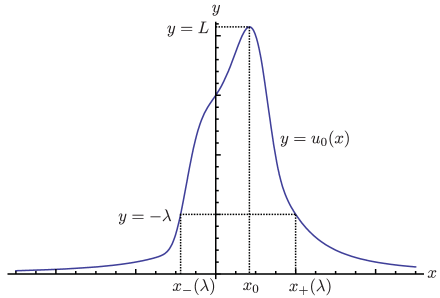
Figure 4. The graph of an admissible initial condition and the turning points $x_{\pm}(\lambda)$.

3.2. Matsuno’s method

In two papers [22, 23], Matsuno proposed a remarkable method to approximate, in the limit $\epsilon\downarrow 0$, the time-independent components of the scattering data for suitable $u_{0}$. His method was based on the conservation laws for the quantities (45). With the use of the more recently obtained trace formulae equating $I_{k}$ as given by (45) with the equivalent formulae (46) [17], several heuristic aspects of the original method given in [22, 23] can be placed on more rigorous footing.

The first key observation made in [22, 23] is that if $u_{0}$ is a smooth function independent of $\epsilon$, then by evaluating the integrals $I_{k}(t)$ at time $t=0$, one sees that they have limiting values as $\epsilon\downarrow 0$. These limits may be obtained simply by solving the recurrence relation (44) with $\epsilon=0$:

(53) $$\lim_{\epsilon\downarrow 0}I_{k}=\int_{\mathbb{R}}u_{0}(x)\mathcal{C}_{+}[u_{0}\mathcal{C}_{+}[u_{0}\mathcal{C}_{+}[\cdots u_{0}\mathcal{C}_{+}[u_{0}]\cdots]]](x)\,dx,\quad k=1,2,3,\dots,$$

where the Cauchy projector $\mathcal{C}_{+}$ occurs $k-1$ times in the integrand. With the use of an identity valid for reasonable complex-valued functions $u_{0}(\cdot)$ and suggested by comparing the conserved quantities generated from the Kaup-Matsuno iteration scheme (44) with those generated via the older scheme of Nakamura [27], one sees that the right-hand side of (53) can be equivalently written in the simple form

(54) $$\lim_{\epsilon\downarrow 0}I_{k}=\frac{1}{k}\int_{\mathbb{R}}u_{0}(x)^{k}\,dx,\quad k=1,2,3,\dots.$$

On the basis of heuristic physical arguments, in [22, 23] Matsuno supposed that for smooth positive initial data $u_{0}$, all moments of the reflection coefficient remain bounded as $\epsilon\downarrow 0$. Adopting this hypothesis, a comparison of (54) with (46) then shows that

(55) $$\lim_{\epsilon\downarrow 0}\epsilon\sum_{n=1}^{N}(-\lambda_{n})^{k-1}=\frac{1}{2\pi k}\int_{\mathbb{R}}u_{0}(x)^{k}\,dx,\quad k=1,2,3,\dots.$$

In particular, taking $k=1$ one obtains

(56) $$\lim_{\epsilon\downarrow 0}\epsilon N=M,$$

where the mass $M$ is defined by (52), so the number of eigenvalues is asymptotically proportional to $1/\epsilon$.

These calculations suggest that the normalized counting measure of eigenvalues may have a limit in a certain sense as $\epsilon\downarrow 0$, perhaps as an absolutely continuous measure with density $F(\lambda)$. Matsuno calculated this density by replacing the left-hand side of (55) with an integral against the unknown density $F(\lambda)$:

(57) $$\int_{-\infty}^{0}(-\lambda)^{k-1}F(\lambda)\,d\lambda=\frac{1}{2\pi k}\int_{\mathbb{R}}u_{0}(x)^{k}\,dx,\quad k=1,2,3,\dots.$$

The problem that remains is then the classical one of constructing the density $F(\lambda)$ from its moments, which are known if the initial condition $u_{0}$ is given.

Matsuno showed that, remarkably, this moment problem can be solved explicitly. He introduced the characteristic function (Fourier transform) of $F$:

(58) $$\hat{F}(\xi):=\int_{-\infty}^{0}F(\lambda)e^{-i\xi\lambda}\,d\lambda,$$

in terms of which, the moment relations (57) become

(59) $$\frac{d^{k-1}\hat{F}}{d\xi^{k-1}}(0)=\frac{i^{k-1}}{2\pi k}\int_{\mathbb{R}}u_{0}(x)^{k}\,dx,\quad k=1,2,3,\dots.$$

Recalling the constants $L$ and $M$ defined by (51) and (52) respectively, it is easy to obtain the estimate

(60) $$\left|\frac{1}{(k-1)!}\frac{d^{k-1}\hat{F}}{d\xi^{k-1}}(0)\right|\leq\frac{ML^{k-1}}{k!}$$

from which it follows that $\hat{F}(\xi)$ is an entire function and hence is equal to its Taylor series about $\xi=0$:

(61) $$\begin{split}\hat{F}(\xi)&=\sum_{k=1}^{\infty}\frac{1}{(k-1)!}\frac{d^{k-1}\hat{F}}{d\xi^{k-1}}(0)\xi^{k-1}\\ &=\sum_{k=1}^{\infty}\frac{(i\xi)^{k-1}}{2\pi k!}\int_{\mathbb{R}}u_{0}(x)^{k}\,dx\\ &=\frac{1}{2\pi i\xi}\sum_{k=1}^{\infty}\int_{\mathbb{R}}\frac{[i\xi u_{0}(x)]^{k}}{k!}\,dx.\end{split}$$

The combined sum and integral is absolutely convergent for all $\xi\in\mathbb{C}$, so the order of operations may be reversed:

(62) $$\hat{F}(\xi)=\frac{1}{2\pi i\xi}\int_{\mathbb{R}}\left(\sum_{k=1}^{\infty}\frac{[i\xi u_{0}(x)]^{k}}{k!}\right)\,dx=\frac{1}{\pi\xi}\int_{\mathbb{R}}e^{i\xi u_{0}(x)/2}\sin\left(\tfrac{1}{2}\xi u_{0}(x)\right)\,dx.$$

By Fourier inversion,

(63) $$F(\lambda)=\frac{1}{2\pi}\lim_{R\uparrow\infty}\int_{-R}^{+R}\hat{F}(\xi)e^{i\xi\lambda}\,d\xi=\lim_{R\uparrow\infty}\int_{-R}^{+R}\int_{\mathbb{R}}\frac{e^{i\xi(\lambda+u_{0}(x)/2)}}{2\pi^{2}\xi}\sin\left(\tfrac{1}{2}\xi u_{0}(x)\right)\,dx\,d\xi.$$

Applying Fubini’s Theorem to reverse the order of integration and then passing to the limit $R\uparrow\infty$, the integral over $\xi$ can be evaluated as the indicator function of an interval:

(64) $$F(\lambda)=\frac{1}{2\pi}\int_{\mathbb{R}}\chi_{[-u_{0}(x),0]}(\lambda)\,dx.$$

This formula shows that $F(\lambda)\equiv 0$ for $\lambda>0$ or $\lambda<-L$. By a “layer-cake” argument we may simplify this formula for $\lambda\in(-L,0)$ as

(65) $$F(\lambda)=\frac{1}{2\pi}\int_{\{x\in\mathbb{R},\;u_{0}(x)>-\lambda\}}dx,\quad-L<\lambda<0.$$

This is Matsuno’s remarkable result. We have presented Matsuno’s method in some detail because it turns out that a key calculation in our analysis of the inverse problem in the zero-dispersion limit reduces to almost the same steps, as we will see shortly. This is worth emphasizing because it provides further evidence that for the BO equation, scattering and inverse-scattering are mathematically very similar operations.

Matsuno’s formula (65) could perhaps be compared with the Bohr-Sommerfeld formula that gives the density of eigenvalues of the Schrödinger operator in the zero-dispersion theory of the KdV equation [20]; aside from a constant factor the Bohr-Sommerfeld formula replaces the unit integrand in (65) with the positive square root $\sqrt{u_{0}(x)+\lambda}$.

While quite severe hypotheses on $u_{0}$ are required for all of the arguments to go through, the formula (65) makes sense under much weaker conditions. In particular, we may interpret (65) for an admissible initial condition, in which case we may express $F(\lambda)$ directly in terms of the turning points $x_{\pm}(\lambda)$:

(66) $$F(\lambda):=\frac{1}{2\pi}\left(x_{+}(\lambda)-x_{-}(\lambda)\right),\quad-L\leq\lambda<0.$$

We take (66) as a definition valid for admissible initial conditions $u_{0}$. Note that

(67) $$\int_{-L}^{0}F(\lambda)\,d\lambda=M,$$

where the mass $M$ is defined by (52).

3.3. Formula for phase constants

The WKB methods recalled by Lax and Levermore [20] to analyze the Schrödinger equation in the forward problem for the zero-dispersion limit of the KdV equation were sufficiently powerful to provide asymptotic formulae for both the discrete spectrum (the Bohr-Sommerfeld formula that is the analogue in the KdV theory of the function $F(\lambda)$ obtained by Matsuno) and also for the “norming constants” that in the KdV theory are the analogues of the phase constants $\{\gamma_{n}\}_{n=1}^{N}$ in the BO theory. However, we have not found a way to apply these methods to the nonlocal operator $\mathcal{L}$, and unfortunately Matsuno’s method does not provide approximations of the phase constants $\{\gamma_{n}\}_{n=1}^{N}$ since they do not enter into the trace formulae.

Our contribution to the theory of the spectral analysis of the nonlocal operator $\mathcal{L}$ in the zero-dispersion limit is to provide a new asymptotic formula for the phase constants. It is difficult to motivate the formula as it arises from the analysis of the inverse problem that we will describe in the next section, but it is nonetheless quite easy to present. If $\lambda<0$ is an eigenvalue of $\mathcal{L}$ with potential $u$ given by an admissible initial condition $u_{0}$, then our approximation to the corresponding phase constant is given in terms of the turning points $x_{\pm}(\lambda)$ as follows:

(68) $$\gamma\approx\gamma(\lambda):=-\frac{1}{2}(x_{+}(\lambda)+x_{-}(\lambda)),\quad-L\leq k<0.$$

Remark 3.1.

Our choice of $\gamma(\lambda)$ in terms of $u_{0}$ is specifically designed to ensure the convergence of $\tilde{u}_{\epsilon}(x,t)$ (to be defined precisely in Definition 3.2 below) at $t=0$ to the given $\epsilon$-independent initial condition $u_{0}$.

3.4. Modification of the Cauchy data

Based on the above considerations, we may now make very precise definitions of formal (not rigorously justified) approximations of the scattering data corresponding to an admissible condition $u_{0}$. The first approximation is to neglect the reflection coefficient by setting

(69) $$\tilde{\beta}(\lambda):=0,\quad\lambda>0.$$

Next we define the exact number of approximate eigenvalues (hopefully also the approximate number of exact eigenvalues) by setting

(70) $$N(\epsilon):=\left\lfloor\frac{M}{\epsilon}\right\rfloor,$$

which in particular implies that

(71) $$\lim_{\epsilon\downarrow 0}\epsilon N(\epsilon)=M.$$

Then we define approximations to the eigenvalues themselves as an ordered set of numbers $\{\tilde{\lambda}_{n}\}_{n=1}^{N(\epsilon)}\subset(-L,0)$ obtained by quantizing the Matsuno eigenvalue density given by (66):

(72) $$\int_{-L}^{\tilde{\lambda}_{n}}F(\lambda)\,d\lambda=\epsilon\left(n-\frac{1}{2}\right),\quad n=1,2,\cdots N(\epsilon).$$

Finally, we define approximations to the corresponding phase constants as numbers $\{\tilde{\gamma}_{n}\}_{n=1}^{N(\epsilon)}$ given precisely by

(73) $$\tilde{\gamma}_{n}:=\gamma(\tilde{\lambda}_{n}),\quad n=1,\dots,N(\epsilon).$$

where $\gamma(\cdot)$ is defined by (68).

Now in our analysis of the Cauchy problem for the BO equation with admissible initial data $u_{0}$ we take a sideways step that is not a priori justified: we simply replace the true solution $u_{\epsilon}(x,t)$ of the Cauchy problem with a family $\tilde{u}_{\epsilon}(x,t)$ of exact solutions of the BO equation (1) with the property that for each $\epsilon>0$ the scattering data for $\tilde{u}_{\epsilon}(x,t)$ at time $t=0$ is exactly the approximate scattering data just defined. This step was also an important part of the method of Lax and Levermore [20]. We formalize this modification of the initial data in the following definition.

Definition 3.2.

Let $u_{0}$ be an admissible initial condition. Then, by $\tilde{u}_{\epsilon}(x,t)$ we mean the exact solution of the BO equation (1) given for each $\epsilon>0$ by the reflectionless inverse-scattering formula

(74) $$\tilde{u}_{\epsilon}(x,t):=2\epsilon\frac{\partial}{\partial x}\Im\{\log(\tilde{\tau}_{\epsilon}(x,t))\},$$

where

(75) $$\tilde{\tau}_{\epsilon}(x,t):=\det\left(\mathbb{I}+i\epsilon^{-1}\tilde{\mathbf{A}}_{\epsilon}\right)$$

and where $\tilde{\mathbf{A}}_{\epsilon}=\tilde{\mathbf{A}}_{\epsilon}(x,t)$ is an $N(\epsilon)\times N(\epsilon)$ Hermitean matrix with elements

(76) $$\tilde{A}_{nm}:=\frac{2i\epsilon\sqrt{\tilde{\lambda}_{n}\tilde{\lambda}_{m}}}{\tilde{\lambda}_{n}-\tilde{\lambda}_{m}},\quad n\neq m$$

and

(77) $$\tilde{A}_{nn}:=-2\tilde{\lambda}_{n}(x+2\tilde{\lambda}_{n}t+\tilde{\gamma}_{n})=-2\tilde{\lambda}_{n}(x+2\tilde{\lambda}_{n}+\gamma(\tilde{\lambda}_{n})).$$

Here the number $N(\epsilon)$ is defined by (70) and the components of the scattering data $\{\tilde{\lambda}_{n}\}_{n=1}^{N(\epsilon)}$ and $\{\tilde{\gamma}_{n}\}_{n=1}^{N(\epsilon)}$ are given explicitly by (72) and (73) respectively.

While it is not the case that $\tilde{u}_{\epsilon}(x,0)=u_{0}(x)$ in general, the relevance of this definition in connection with the Cauchy problem with initial condition $u_{0}$ is a consequence of Corollary 1.1 which guarantees convergence in the mean square sense of $\tilde{u}_{\epsilon}(\cdot,0)$ to $u_{0}(\cdot)$ as $\epsilon\downarrow 0$.

The proof of Theorem 1.1 will be given below in §4. Before embarking on that we note that Definition 3.1 implies a number of properties of the functions $F$ and $\gamma$ that will be useful later, so we take the opportunity to record these here. Note that $F$ and $\gamma$ will frequently occur in the context of the following functions:

(78) $$D(\lambda;x,t):=-2\lambda(x+2\lambda t+\gamma(\lambda)),\quad-L<\lambda<0,$$

and

(79) $$\varphi(\lambda):=\sqrt{-\lambda F(\lambda)},\quad-L<\lambda<0.$$

Lemma 3.1.

Let $u_{0}$ be an admissible initial condition with decay exponent $q>1$, and let $F:[-L,0)\to\mathbb{R}$ be defined by (66) and $\gamma:[-L,0)\to\mathbb{R}$ be defined by (68). Then $F$ and $\gamma$ both belong to $C^{(1)}(-L,0)$ and $F$ and $F^{\prime}$ are strictly positive on this open interval. Also, there exists a sufficiently small constant $\delta>0$ and positive constants $C_{-L}$ and $C_{0}$ such that

(80) $$\frac{1}{2}C_{-L}\sqrt{L+\lambda}<F(\lambda)<C_{-L}\sqrt{L+\lambda},$$

and

(81) $$\frac{1}{4}\frac{C_{-L}}{\sqrt{L+\lambda}}<F^{\prime}(\lambda)<\frac{1}{2}\frac{C_{-L}}{\sqrt{L+\lambda}}$$

both hold for $-L<\lambda<-L+\delta$, while

(82) $$\frac{1}{2}C_{0}(-\lambda)^{-1/q}<F(\lambda)<C_{0}(-\lambda)^{-1/q},$$

and

(83) $$\frac{1}{2}\frac{C_{0}}{q}(-\lambda)^{-1/q-1}<F^{\prime}(\lambda)<\frac{C_{0}}{q}(-\lambda)^{-1/q-1}$$

both hold for $-\delta<\lambda<0$. Also,

(84) $$|\gamma(\lambda)+x_{0}|\leq\pi F(\lambda)\quad\text{and}\quad|\gamma^{\prime}(\lambda)|\leq\pi F^{\prime}(\lambda),\quad-L\leq\lambda<0,$$

inequalities that when combined with (80)–(83) imply obvious upper bounds for $|\gamma(\lambda)+x_{0}|$ and $|\gamma^{\prime}(\lambda)|$.

In particular, these estimates show that $F(\lambda)$ is integrable, and $\varphi(\lambda)$ and $D(\lambda;x,t)$ (and hence also $\lambda x_{\pm}(\lambda)$) are bounded, and that with $\sigma=\min(\tfrac{1}{2},1-\tfrac{1}{q})\in(0,1)$, $\varphi(\cdot)$ is Hölder continuous with exponent $\sigma/2$ while $D(\cdot;x,t)$ is Hölder continuous with exponent $\sigma$ uniformly for $(x,t)$ in compact sets, on $(-L,0)$.

Proof.

The turning points $x_{\pm}(\lambda)$ are clearly of class $C^{(1)}(-L,0)$, by definition $x_{+}(\lambda)>x_{0}>x_{-}(\lambda)$ on this open interval, and moreover $x_{+}(\lambda)$ is strictly increasing while $x_{-}(\lambda)$ is strictly decreasing on $(-L,0)$. These facts immediately imply the desired basic smoothness properties of $F$ and $\gamma$, and the positivity and monotonicity of $F$, as well as the inequalities (84).

Since $u_{0}(x_{0})=L$ and $u_{0}^{\prime}(x_{0})=0$, the $C^{(2)}(\mathbb{R})$ function $u_{0}$ satisfies

(85) $$\lim_{x\to x_{0}}\frac{u_{0}(x)-L}{(x-x_{0})^{2}}=\frac{u^{\prime\prime}_{0}(x_{0})}{2}\quad\text{and}\quad\lim_{x\to x_{0}}\frac{u^{\prime}_{0}(x)}{x-x_{0}}=u^{\prime\prime}_{0}(x_{0}).$$

Using these together with the inequality $u^{\prime\prime}_{0}(x_{0})<0$, the definition of $x_{\pm}(\lambda)$ as branches of the inverse function of $u_{0}$ shows that

(86) $$\lim_{\lambda\downarrow-L}\frac{\pm(x_{\pm}(\lambda)-x_{0})}{\sqrt{L+\lambda}}=\sqrt{\frac{2}{-u^{\prime\prime}_{0}(x_{0})}}\quad\text{and}\quad\lim_{\lambda\downarrow-L}\pm x^{\prime}_{\pm}(\lambda)\sqrt{L+\lambda}=\sqrt{\frac{1}{-2u^{\prime\prime}_{0}(x_{0})}}.$$

Using these relations in (66) and (68) establishes the existence of the limits

(87) $$\lim_{\lambda\downarrow-L}\frac{F(\lambda)}{\sqrt{L+\lambda}}=\frac{1}{\pi}\sqrt{\frac{2}{-u^{\prime\prime}_{0}(x_{0})}}\quad\text{and}\quad\lim_{\lambda\downarrow-L}F^{\prime}(\lambda)\sqrt{L+\lambda}=\frac{1}{2\pi}\sqrt{\frac{2}{-u^{\prime\prime}_{0}(x_{0})}},$$

which prove the two-sided estimates (80) and (81).

Next, note that the decay conditions (49) and (50) for $u_{0}$ and its derivative together imply that

(88) $$\lim_{\lambda\uparrow 0}x_{\pm}(\lambda)(-\lambda)^{\frac{1}{q}}=\pm\left(\mp\frac{C_{\pm}}{q}\right)^{\frac{1}{q}}\quad\text{and}\quad\lim_{\lambda\uparrow 0}x_{\pm}^{\prime}(-\lambda)^{\tfrac{1}{q}+1}=\pm\frac{1}{q}\left(\mp\frac{C_{\pm}}{q}\right)^{\tfrac{1}{q}},$$

where $\mp C_{\pm}$ are the positive constants in (49) and (50). It follows from (66) that

(89) $$\lim_{\lambda\uparrow 0}F(\lambda)(-\lambda)^{\frac{1}{q}}=\frac{1}{2\pi}\left[\left(-\frac{C_{+}}{q}\right)^{\frac{1}{q}}+\left(\frac{C_{-}}{q}\right)^{\frac{1}{q}}\right],$$

which proves (82) and

(90) $$\lim_{\lambda\uparrow 0}F^{\prime}(\lambda)(-\lambda)^{\frac{1}{q}+1}=\frac{1}{2\pi q}\left[\left(-\frac{C_{+}}{q}\right)^{\frac{1}{q}}+\left(\frac{C_{-}}{q}\right)^{\frac{1}{q}}\right],$$

which proves (83). ∎

4. The Inverse-Scattering Problem in the Zero-Dispersion Limit

In this section, we provide the proof of Theorem 1.1.

4.1. Basic strategy. Outline of proof

According to Definition 3.2, $\tilde{u}_{\epsilon}(x,t)$ is expressed in terms of the determinant $\tilde{\tau}_{\epsilon}$ as follows:

(91) $$\tilde{u}_{\epsilon}(x,t)=\frac{\partial\tilde{U}_{\epsilon}}{\partial x}(x,t),\quad\tilde{U}_{\epsilon}(x,t)=2\epsilon\Im\{\log(\tilde{\tau}_{\epsilon}(x,t))\}.$$

As the logarithm of a complex-valued quantity is involved, $\tilde{U}_{\epsilon}(x,t)$ is only defined modulo $4\pi\epsilon$ for each $(x,t)$, and naturally one should choose the appropriate branch for each $(x,t)$ to achieve continuity. We do this concretely in equation (93) below.

At this very early point our analysis must take a very different path than that followed by Lax and Levermore [20] in their study of the zero-dispersion limit for the KdV equation. Indeed, the expansion of $\tilde{\tau}_{\epsilon}$ in principal minors that is at the heart of the Lax-Levermore method would be a poor choice in this situation. One reason for this is simply that the principal-minors expansion of $\tilde{\tau}_{\epsilon}(x,t)$ consists of complex-valued terms of indefinite phase, so the sum cannot be easily estimated by its largest term. But a more important reason is that the formula (91) for $\tilde{U}_{\epsilon}(x,t)$ involves not $\log(\tilde{\tau}_{\epsilon})$ but rather $\Im\{\log(\tilde{\tau}_{\epsilon})\}$, that is, we require an estimate of the phase of the determinant and we are not interested in its magnitude.

So instead of expanding the determinant as a sum, we write it as a product. Let $\{\alpha_{n}\}_{n=1}^{N(\epsilon)}$ be the real eigenvalues of $\tilde{\mathbf{A}}_{\epsilon}(x,t)$. Then the corresponding eigenvalues of $\mathbb{I}+i\epsilon^{-1}\tilde{\mathbf{A}}_{\epsilon}(x,t)$ are of course $\{1+i\epsilon^{-1}\alpha_{n}\}_{n=1}^{N(\epsilon)}$, so we may expand $\tilde{\tau}_{\epsilon}$ as a product over eigenvalues in the form:

(92) $$\tilde{\tau}_{\epsilon}(x,t)=\prod_{n=1}^{N(\epsilon)}\left(1+i\epsilon^{-1}\alpha_{n}\right).$$

This yields a suggestive formula for $\tilde{U}_{\epsilon}(x,t)$ in terms of the eigenvalues of $\tilde{\mathbf{A}}_{\epsilon}$:

(93) $$\tilde{U}_{\epsilon}(x,t):=\epsilon\sum_{n=1}^{N(\epsilon)}2\arctan\left(\epsilon^{-1}\alpha_{n}\right).$$

Here $-\pi/2<\arctan(\cdot)<\pi/2$, so in particular by this definition we have made an unambiguous choice of the branch of the logarithm. This formula seems at first not to be of much use because, unlike the principal minor determinants in the Lax-Levermore method which can be written explicitly in terms of the matrix elements, the eigenvalues of $\tilde{\mathbf{A}}_{\epsilon}$ are only implicitly known. However, numerical experiments suggest that some structure emerges in the limit $\epsilon\downarrow 0$. Indeed, the plots shown in Figure 5

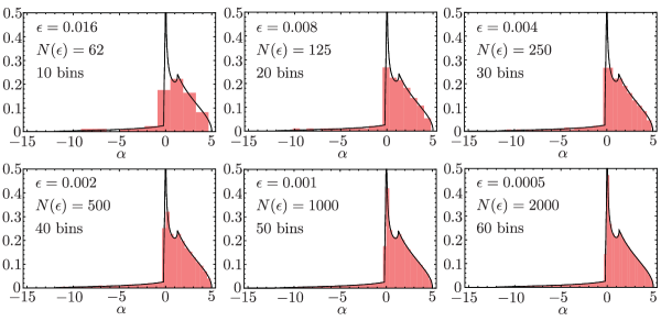
Figure 5. Histograms of eigenvalues of $\tilde{\mathbf{A}}_{\epsilon}$ corresponding to the initial condition $u_{0}(x):=2(1+x^{2})^{-1}$, $x=5$, and $t=2$, normalized to have total area $M=1$, compared with the density $G(\alpha;x,t)$ of the limiting absolutely continuous measure $\mu$.

provide good evidence that the normalized (to mass $M$) counting measures $\mu_{\epsilon}$ given for $\epsilon>0$ by

(94) $$\mu_{\epsilon}:=\frac{M}{N(\epsilon)}\sum_{n=1}^{N(\epsilon)}\delta_{\alpha_{n}},\quad\text{$\{\alpha_{n}\}_{n=1}^{N(\epsilon)}$ eigenvalues of $\tilde{\mathbf{A}}_{\epsilon}$}$$

might converge in some sense to a measure $\mu$ having a density $G(\alpha;x,t)$. This convergence suggests further that the formula (93) could be interpreted as a Riemann sum, for the integral of $\pi\,\mathrm{sgn}(\alpha)$ (the pointwise limit as $\epsilon\downarrow 0$ of the summand) against the limiting measure $\mu$. We will prove that indeed $\tilde{U}_{\epsilon}(x,t)$ converges, uniformly with respect to $x$ and $t$ in compact sets, to a limit function $U(x,t)$ given by such an integral in the limit $\epsilon\downarrow 0$.

To obtain an effective formula for $U(x,t)$ we need to analyze the asymptotic behavior of the measures $\mu_{\epsilon}$. This part of our analysis is modeled after the work of Wigner [32, 33] on the statistical distribution of eigenvalues of random Hermitian matrices with independent and identically distributed matrix elements. Like Wigner, we use the method of moments because while the measures themselves are not easy to express in terms of the matrix elements, their moments are:

(95) $$\int_{\mathbb{R}}\alpha^{p}\,d\mu_{\epsilon}(\alpha)=\frac{M}{N(\epsilon)}\sum_{n=1}^{N(\epsilon)}\alpha_{n}^{p}=\frac{M}{N(\epsilon)}\mathrm{tr}(\tilde{\mathbf{A}}_{\epsilon}^{p}),\quad p=0,1,2,\dots.$$

We prove the existence of the limit of the right-hand side in equation (95) as $\epsilon\downarrow 0$ for every $p$ using the fact that for small $\epsilon$ the matrix $\tilde{\mathbf{A}}_{\epsilon}$ concentrates near the diagonal, where it can be approximated by the product of a diagonal matrix and the Toeplitz matrix corresponding to the symbol $f(\theta):=i(\pi-\theta)$, $0<\theta<2\pi$ (of singular Fisher-Hartwig type due to jump discontinuities). The result of this asymptotic analysis of moments is the following Proposition, the proof of which will be given below in §4.2.

Proposition 4.1.

For each nonnegative integer $p$,

(96) $$\lim_{\epsilon\downarrow 0}\int_{\mathbb{R}}\alpha^{p}\,d\mu_{\epsilon}(\alpha)=Q_{p},$$

with the limit being uniform with respect to $(x,t)$ in any compact set, where

(97) $$Q_{p}:=\frac{1}{2\pi(p+1)}\int_{-L}^{0}\left[\left(x+2\lambda t-x_{-}(\lambda)\right)^{p+1}-\left(x+2\lambda t-x_{+}(\lambda)\right)^{p+1}\right](-2\lambda)^{p}\,d\lambda.$$

Given these limiting moments, the next task is to establish the existence of a corresponding limiting measure $\mu$ with these moments, and to prove the existence of the limit $\tilde{U}_{\epsilon}(x,t)\to U(x,t)$. A remarkable feature of this analysis is that the solution of the moment problem for $\mu$ is carried out by virtually the same procedure as Matsuno used to obtain the function $F(\lambda)$ from $u_{0}$ (see §3.2). Our result is the following Proposition, that will be proved in all details in §4.3.

Proposition 4.2.

Uniformly for $(x,t)$ in compact sets,

(98) $$\lim_{\epsilon\downarrow 0}\tilde{U}_{\epsilon}(x,t)=U(x,t),$$

where

(99) $$U(x,t):=\int_{\mathbb{R}}\pi\,\mathrm{sgn}(\alpha)\,d\mu(\alpha)$$

and where $\mu$ is an absolutely continuous measure of mass $M$ with density $G(\alpha;x,t)$, and

(100) $$G(\alpha;x,t):=-\frac{1}{4\pi}\int_{-L}^{0}\chi_{[-2\lambda(x+2\lambda t-x_{+}(\lambda)),-2\lambda(x+2\lambda t-x_{-}(\lambda))]}(\alpha)\frac{d\lambda}{\lambda}.$$

Here, $\chi_{[a,b]}(z)$ denotes the indicator function of the interval $[a,b]$.

The limiting measure $\mu$ is the closest analogue in the zero-dispersion theory of the BO equation of the equilibrium (or extremal) measure arising in the Lax-Levermore theory of the KdV equation. But a significant difference is that in this case the measure $\mu$ is specified explicitly rather than implicitly as the solution of a variational problem.

The region of integration in the double integral obtained by combining (100) with (99) is illustrated for three different values of $(x,t)$ in Figure 6.

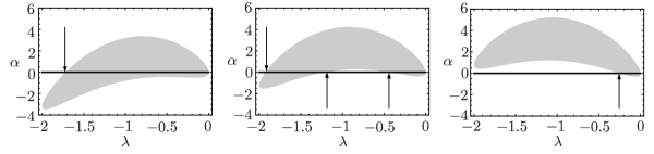
Figure 6. The region of integration $-2\lambda(x+2\lambda t-x_{+}(\lambda))<\alpha<-2\lambda(x+2\lambda t-x_{-}(\lambda))$ for $u_{0}(x)=2(1+x^{2})^{-1}$ with $t=0.7$. Left: $x=2$ (to the left of the oscillatory region for $u_{\epsilon}(x,t)$). Center: $x=2.5$ (within the oscillatory region for $u_{\epsilon}(x,t)$). Right: $x=3$ (to the right of the oscillatory region for $u_{\epsilon}(x,t)$). The line $\alpha=0$ of discontinuity of the integrand is superimposed, and the intersections of the boundary with this line are indicated with arrows.

The points where the boundary curves of this region intersect the line $\alpha=0$ (where the integrand is discontinuous) obviously will play an important role in the differentiation of $U(x,t)$ with respect to $x$. Moreover, these intersection points correspond (simply by changing the sign) to the branches of the multivalued solution of Burgers’ equation with initial data $u_{0}$. This explains their appearance in the formula for the weak limit of $u_{\epsilon}(x,t)$. All details of this calculation will be given in §4.4, which will complete the proof of Theorem 1.1.

4.2. Asymptotics of traces of powers of $\tilde{\mathbf{A}}_{\epsilon}$. Proof of Proposition 4.1

The definition (72) implies that where $F(\lambda)$ is bounded and bounded away from zero, the numbers $\{\tilde{\lambda}_{n}\}_{n=1}^{N(\epsilon)}$ are locally nearly equally spaced, but they are more dilute near the “soft edge” of the spectrum $\lambda=-L$ and more dense near the “hard edge” of the spectrum $\lambda=0$. Taking into account the soft edge behavior we may obtain a uniform estimate:

Lemma 4.1.

There is a constant $C_{\lambda}>0$ independent of $\epsilon$ such that

(101) $$|\tilde{\lambda}_{n}-\tilde{\lambda}_{m}|\leq C_{\lambda}\epsilon^{2/3}|n-m|^{2/3}$$

holds for all $n$ and $m$ between $1$ and $N(\epsilon)$.

Proof.

Since $F$ is a monotone increasing function with $F(-L)=0$, it is bounded away from zero except in a right-neighborhood of $\lambda=-L$. Using the lower bound given in (80) from Lemma 3.1 we obtain a lower bound $F(\lambda)\geq C\sqrt{L+\lambda}$ valid uniformly for $-L<\lambda<0$ with $0<C\leq C_{-L}/2$. Then, using the definition (72) we have (assuming $n\geq m$ without loss of generality)

(102) $$\epsilon|n-m|=\int_{\tilde{\lambda}_{m}}^{\tilde{\lambda}_{n}}F(\lambda)\,d\lambda\geq C\int_{\tilde{\lambda}_{m}}^{\tilde{\lambda}_{n}}\sqrt{L+\lambda}\,d\lambda\geq C\int_{0}^{|\tilde{\lambda}_{n}-\tilde{\lambda}_{m}|}\sqrt{\xi}\,d\xi=\frac{2C}{3}|\tilde{\lambda}_{n}-\tilde{\lambda}_{m}|^{3/2},$$

so the desired inequality follows with $C_{\lambda}:=(2C/3)^{-2/3}$. ∎

We decompose the matrix $\tilde{\mathbf{A}}_{\epsilon}$ into a sum $\tilde{\mathbf{A}}_{\epsilon}=\mathbf{D}+\mathbf{H}$ of its diagonal part

(103) $$\mathbf{D}:=\mathrm{diag}(D_{1},D_{2},\dots,D_{N(\epsilon)}),\quad D_{k}:=D(\tilde{\lambda}_{k};x,t),$$

where $D(\lambda;x,t)$ is defined by (78), and its off-diagonal part $\mathbf{H}$ whose matrix elements are given by

(104) $$H_{nm}=\frac{2i\epsilon\sqrt{\tilde{\lambda}_{n}\tilde{\lambda}_{m}}}{\tilde{\lambda}_{n}-\tilde{\lambda}_{m}},\quad\text{for $n\neq m$, and $H_{nn}=0$.}$$

We also will soon need the quantities $\{\varphi_{n}\}_{n=1}^{N(\epsilon)}$ defined by

(105) $$\varphi_{n}:=\varphi(\tilde{\lambda}_{n}),\quad n=1,\dots,N(\epsilon),$$

where $\varphi(\lambda)$ is given by (79).

Lemma 4.2.

There is a constant $C_{\varphi}>0$ and for each $R>0$ there is a constant $C_{D,R}>0$ such that

(106) $$|\varphi_{n}|\leq C_{\varphi}$$

and

(107) $$\sup_{x^{2}+t^{2}\leq R^{2}}|D_{n}|\leq C_{D,R}$$

both hold for all $\epsilon>0$ and all $n$ between $1$ and $N(\epsilon)$. Also,

(108) $$|\varphi_{n}-\varphi_{m}|\leq C_{\varphi}\epsilon^{\sigma/3}|n-m|^{\sigma/3}$$

and

(109) $$\sup_{x^{2}+t^{2}\leq R^{2}}|D_{n}-D_{m}|\leq C_{D,R}\epsilon^{\sigma/3}|n-m|^{\sigma/3}$$

both hold for all $\epsilon>0$ and for all $n$ and $m$ between $1$ and $N(\epsilon)$. Here $\sigma$ is the positive Hölder exponent of Lemma 3.1.

Proof.

This is an easy consequence of the Hölder continuity of $\varphi(\cdot)$ and $D(\cdot;x,t)$ guaranteed by Lemma 3.1, and of the spacing estimate for $\{\tilde{\lambda}_{k}\}_{k=1}^{N(\epsilon)}$ given in Lemma 4.1. In fact, since $D$ is Hölder continuous with exponent $\sigma$ while $\varphi$ has exponent $\sigma/2$ the most natural bound for $|D_{n}-D_{m}|$ is proportional to $\epsilon^{2\sigma/3}|n-m|^{2\sigma/3}$, and to obtain (109) we use the fact that $\epsilon|n-m|\leq 2\epsilon N(\epsilon)$ is uniformly bounded to reduce the exponent to $\sigma/3$. ∎

Lemma 4.3.

There is a constant $C_{H}>0$ such that

(110) $$\left|(n-m)H_{nm}\right|\leq C_{H}$$

and

(111) $$\left|(n-m)H_{nm}-2i\varphi_{n}\varphi_{m}\right|\leq C_{H}\epsilon^{\sigma/3}|n-m|^{\sigma/3}$$

both hold for all $\epsilon>0$ and all $n\neq m$ between $1$ and $N(\epsilon)$. Again, $\sigma>0$ is the Hölder exponent of Lemma 3.1.

Proof.

Suppose without loss of generality that $n>m$, implying that $\tilde{\lambda}_{m}<\tilde{\lambda}_{n}<0$. Then

(112) $$\begin{split}-i(n-m)H_{nm}&=2\sqrt{-\tilde{\lambda}_{n}}\sqrt{-\tilde{\lambda}_{m}}\frac{\epsilon(n-m)}{\tilde{\lambda}_{n}-\tilde{\lambda}_{m}}\\ &\leq([-\tilde{\lambda}_{n}]+[-\tilde{\lambda}_{m}])\frac{\epsilon(n-m)}{\tilde{\lambda}_{n}-\tilde{\lambda}_{m}}\\ &=\epsilon(n-m)-2\tilde{\lambda}_{n}\frac{\epsilon(n-m)}{\tilde{\lambda}_{n}-\tilde{\lambda}_{m}}.\end{split}$$

Now, recalling the definition (72) of the numbers $\{\tilde{\lambda}_{k}\}_{k=1}^{N(\epsilon)}$ and applying the Mean Value Theorem we may write the latter difference quotient as $F(\xi)$ for some $\xi$ with $\tilde{\lambda}_{m}\leq\xi\leq\tilde{\lambda}_{n}$, and since $F$ is increasing we have $F(\xi)\leq F(\tilde{\lambda}_{n})$, so

(113) $$-i(n-m)H_{nm}\leq 2\epsilon(n-m)-2\tilde{\lambda}_{n}F(\tilde{\lambda}_{n})=2\epsilon(n-m)+2\varphi_{n}^{2},$$

where we have also replaced $\epsilon(n-m)$ with $2\epsilon(n-m)$. On the other hand, we may write

(114) $$-i(n-m)H_{nm}=2\epsilon(n-m)\frac{\sqrt{-\tilde{\lambda}_{n}}\sqrt{-\tilde{\lambda}_{m}}+\tilde{\lambda}_{m}}{\tilde{\lambda}_{n}-\tilde{\lambda}_{m}}-2\tilde{\lambda}_{m}\frac{\epsilon(n-m)}{\tilde{\lambda}_{n}-\tilde{\lambda}_{m}}.$$

Again the difference quotient may be replaced by $F(\xi)\geq F(\tilde{\lambda}_{m})$, and since

(115) $$\frac{\sqrt{-\tilde{\lambda}_{n}}\sqrt{-\tilde{\lambda}_{m}}}{\tilde{\lambda}_{n}-\tilde{\lambda}_{m}}=-\frac{\sqrt{-\tilde{\lambda}_{m}}}{\sqrt{\tilde{\lambda}_{n}}+\sqrt{\tilde{\lambda}_{m}}}\geq-1,$$

we obtain

(116) $$-i(n-m)H_{nm}\geq-2\epsilon(n-m)-2\tilde{\lambda}_{m}F(\tilde{\lambda}_{m})=-2\epsilon(n-m)+2\varphi_{m}^{2}.$$

Combining (113) and (116) gives

(117) $$\left|(n-m)H_{nm}-2i\varphi_{n}\varphi_{m}\right|\leq 2\epsilon|n-m|+2\max\{\varphi_{n},\varphi_{m}\}|\varphi_{n}-\varphi_{m}|,$$

and then applying Lemma 4.2 we obtain

(118) $$\left|(n-m)H_{nm}-2i\varphi_{n}\varphi_{m}\right|\leq 2\epsilon|n-m|+2C_{\varphi}^{2}\epsilon^{\sigma/3}|n-m|^{\sigma/3}.$$

Now, $0\leq\epsilon|n-m|\leq 2\epsilon N(\epsilon)$, and this upper bound has a limit as $\epsilon\downarrow 0$, so $\epsilon|n-m|$ is nonnegative and bounded. Since $\sigma\leq 3$ we have therefore proved (111). Since $\varphi_{n}\varphi_{m}$ and $\epsilon|n-m|$ are bounded, (110) then follows from (111). ∎

For any nonnegative integer power $p$, the $p$th moment of the measure $\mu_{\epsilon}$ can be written in terms of $\mathbf{D}$ and $\mathbf{H}$ with the use of (95):

(119) $$\int_{\mathbb{R}}\alpha^{p}d\mu_{\epsilon}(\alpha)=\sum_{j=0}^{p}Z_{pj},$$

where $Z_{pj}$ contains the contribution to the trace coming from products of matrices involving exactly $j$ factors of $\mathbf{H}$:

(120) $$Z_{pj}:=\frac{M}{N(\epsilon)}\mathop{\sum_{d_{1}+d_{2}+\cdots+d_{s}=p-j}}_{h_{1}+h_{2}+\cdots+h_{s}=j}\mathrm{tr}\left(\mathbf{D}^{d_{1}}\mathbf{H}^{h_{1}}\cdots\mathbf{D}^{d_{s}}\mathbf{H}^{h_{s}}\right),$$

and where $d_{1}\geq 0$ and $h_{s}\geq 0$, while $d_{k}>0$ for $2\leq k\leq s$ and $h_{k}>0$ for $1\leq k\leq s-1$. Since $p$ is a fixed number, it will suffice to compute the limit of $Z_{pj}$ as $\epsilon\downarrow 0$ for $j=0,\dots,p$. Actually, it will be enough to consider even values of $j$ as the following result shows.

Lemma 4.4.

If $j$ is an odd number, then $Z_{pj}=0$.

Proof.

Since $\mathrm{tr}(\mathbf{M})=\mathrm{tr}(\mathbf{M}^{\mathsf{T}})$ for all square matrices $\mathbf{A}$,

(121) $$\begin{split}\frac{N(\epsilon)}{M}Z_{pj}=&\mathop{\sum_{d_{1}+d_{2}+\cdots+d_{s}=p-j}}_{h_{1}+h_{2}+\cdots+h_{s}=j}\mathrm{tr}\left(\left(\mathbf{D}^{d_{1}}\mathbf{H}^{h_{1}}\cdots\mathbf{D}^{d_{s}}\mathbf{H}^{h_{s}}\right)^{\mathsf{T}}\right)\\ =&(-1)^{j}\mathop{\sum_{d_{1}+d_{2}+\cdots+d_{s}=p-j}}_{h_{1}+h_{2}+\cdots+h_{s}=j}\mathrm{tr}\left(\mathbf{H}^{h_{s}}\mathbf{D}^{d_{s}}\cdots\mathbf{H}^{h_{1}}\mathbf{D}^{d_{1}}\right)\end{split}$$

where in the second line we have used the facts that $\mathbf{D}^{\mathsf{T}}=\mathbf{D}$ and $\mathbf{H}^{\mathsf{T}}=-\mathbf{H}$. By relabeling the terms in the sum we therefore obtain

(122) $$\frac{N(\epsilon)}{M}Z_{pj}=(-1)^{j}\frac{N(\epsilon)}{M}Z_{pj}.$$

Since $N(\epsilon)>0$ and $M<\infty$, the desired result follows. ∎

An important role will be played below by the Toeplitz (discrete convolution) operator $\mathcal{T}_{f}:\ell^{2}(\mathbb{Z})\to\ell^{2}(\mathbb{Z})$ defined by

(123) $$\left(\mathcal{T}_{f}c\right)_{n}:=\sum_{m\in\mathbb{Z}}f_{n-m}c_{m},\quad\{c_{m}\}_{m\in\mathbb{Z}}\in\ell^{2}(\mathbb{Z}),$$

where $\{f_{n}\}_{n\in\mathbb{Z}}\in\ell^{2}(\mathbb{Z})$ is the sequence

(124) $$f_{n}:=\begin{cases}n^{-1},\quad&n\neq 0\\ 0,\quad&n=0.\end{cases}$$

Lemma 4.5.

For any even positive integer $j$, we have

(125) $$\sum_{n_{2},\dots,n_{j}\in\mathbb{Z}}f_{-n_{2}}\left[\prod_{\ell=2}^{j-1}f_{n_{\ell}-n_{\ell+1}}\right]f_{n_{j}}=\frac{(i\pi)^{j}}{j+1},$$

where the $j-1$-fold infinite sum converges absolutely.

Proof.

Note that since $\{f_{n}\}_{n\in\mathbb{Z}}\in\ell^{2}(\mathbb{Z})$, $\{g_{n}\}_{n\in\mathbb{Z}}\in\ell^{2}(\mathbb{Z})$ as well, where $g_{n}:=|f_{n}|$ for all $n\in\mathbb{Z}$. The corresponding Fourier series converge in the mean-square sense to functions $f(\cdot)$ and $g(\cdot)$ in $L^{2}[0,2\pi]$:

(126) $$f(\theta):=\sum_{n\in\mathbb{Z}}f_{n}e^{in\theta}=i(\pi-\theta),\quad 0<\theta<2\pi$$

and

(127) $$g(\theta):=\sum_{n\in\mathbb{Z}}g_{n}e^{in\theta}=-\log(2(1-\cos(\theta))),\quad 0<\theta<2\pi.$$

First we establish the absolute convergence of the series on the left-hand side of (125). Using (123), observe that

(128) $$\sum_{n_{2},\dots,n_{j}\in\mathbb{Z}}|f_{-n_{2}}|\left[\prod_{\ell=2}^{j-1}|f_{n_{\ell}-n_{\ell+1}}|\right]|f_{n_{j}}|=\left(\mathcal{T}_{g}^{j-1}g\right)_{0}$$

where $\mathcal{T}_{g}$ is the Toeplitz operator associated with the sequence $\{g_{n}\}_{n\in\mathbb{Z}}$. Now, $g(\cdot)$ has a logarithmic singularity at $\theta=0\pmod{2\pi}$, but this is sufficiently mild that $g(\cdot)^{m}\in L^{2}[0,2\pi]\subset L^{1}[0,2\pi]$ for any positive integer power $m$. Now for any function $k(\cdot)\in L^{2}[0,2\pi]$, the corresponding Fourier coefficients are

(129) $$k_{n}:=\frac{1}{2\pi}\int_{0}^{2\pi}k(\theta)e^{-in\theta}\,d\theta,$$

so in particular we see that $(\mathcal{T}_{g}^{j-1}g)_{0}$ is the average value of the function whose Fourier coefficients are $\{(\mathcal{T}_{g}^{j-1}g)_{n}\}_{n\in\mathbb{Z}}$. But by the convolution theorem:

(130) $$w_{n}:=\sum_{m\in\mathbb{Z}}u_{n-m}v_{m}\quad\quad\Longleftrightarrow\quad\quad w(\theta)=u(\theta)v(\theta),$$

so it follows that

(131) $$\left(\mathcal{T}_{g}^{j-1}g\right)_{0}=\frac{1}{2\pi}\int_{0}^{2\pi}g(\theta)^{j}\,d\theta$$

which is finite because $g(\cdot)^{j}\in L^{1}[0,2\pi]$.

Now we find the exact value of the $j-1$-fold infinite sum by the same reasoning:

(132) $$\sum_{n_{2},\dots,n_{j}\in\mathbb{Z}}f_{-n_{2}}\left[\prod_{\ell=2}^{j-1}f_{n_{\ell}-n_{\ell+1}}\right]f_{n_{j}}=\left(\mathcal{T}_{f}^{j-1}f\right)_{0}=\frac{1}{2\pi}\int_{0}^{2\pi}f(\theta)^{j}\,d\theta,$$

and by direct calculation using (126),

(133) $$\frac{1}{2\pi}\int_{0}^{2\pi}f(\theta)^{j}\,d\theta=\frac{1}{2\pi}\int_{0}^{2\pi}[i(\pi-\theta)]^{j}\,d\theta=\frac{(i\pi)^{j}}{j+1}$$

for $j$ even (the integral vanishes by symmetry for $j$ odd). ∎

Now we consider separately each of the terms in $Z_{pj}$ for $j$ even.

Lemma 4.6.

If $j$ is an even number and $h_{1}+\cdots+h_{s}=j$ while $d_{1}+\cdots+d_{s}=p-j$, then

(134) $$\lim_{\epsilon\downarrow 0}\frac{M}{N(\epsilon)}\mathrm{tr}\left(\mathbf{D}^{d_{1}}\mathbf{H}^{h_{1}}\cdots\mathbf{D}^{d_{s}}\mathbf{H}^{h_{s}}\right){}=\frac{(2\pi)^{j}}{j+1}\int_{-L}^{0}D(\lambda;x,t)^{p-j}\varphi(\lambda)^{2j}F(\lambda)\,d\lambda,$$

with the limit being uniform with respect to $(x,t)$ in any compact set.

Proof.

Recalling the matrix elements $D_{n}$ and $H_{nm}$ of $\mathbf{D}$ and $\mathbf{H}$ respectively, we have

(135) $$\mathrm{tr}\left(\mathbf{D}^{d_{1}}\mathbf{H}^{h_{1}}\cdots\mathbf{D}^{d_{s}}\mathbf{H}^{h_{s}}\right)=\sum_{a_{1},a_{2},\dots,a_{j}=1}^{N(\epsilon)}\left[\prod_{i=1}^{j}D_{a_{i}}^{m_{i}}\right]\left[\prod_{\ell=1}^{j-1}H_{a_{\ell}a_{\ell+1}}\right]H_{a_{j}a_{1}},$$

where the exponents $m_{1},\dots,m_{j}$ are given by

(136) $$m_{i}:=\begin{cases}d_{1},\quad&i=1\\ d_{b+1},\quad&i=1+h_{1}+h_{2}+\cdots+h_{b}\quad\text{for some $0<b<s$}\\ 0,\quad&\text{otherwise}.\end{cases}$$

Note that $m_{1}+m_{2}+\cdots+m_{j}=d_{1}+d_{2}+\cdots d_{s}=p-j$.

Now, the matrix element $H_{nm}$ is relatively small unless $n\approx m$, and this suggests that the $j$-fold sum in (135) should concentrate near the diagonal, where $a_{k}=a_{1}$ for all $k$. Making this precise, given any $r>0$ we will first show that

(137) $$\lim_{\epsilon\downarrow 0}Z_{\mathrm{OD}}(\epsilon)=0,$$

where

(138) $$Z_{\mathrm{OD}}(\epsilon):=\frac{M}{N(\epsilon)}\mathop{\sum_{a_{1},a_{2},\dots,a_{j}=1}^{N(\epsilon)}}_{\exists k:|a_{k}-a_{1}|>\epsilon^{-r}}\left[\prod_{i=1}^{j}D_{a_{i}}^{m_{i}}\right]\left[\prod_{\ell=1}^{j-1}H_{a_{\ell}a_{\ell+1}}\right]H_{a_{j}a_{1}},$$

with the limit being uniform for $(x,t)$ in compact sets. Indeed, if $x^{2}+t^{2}\leq R^{2}$, then using (107) from Lemma 4.2 and (110) from Lemma 4.3 we obtain

(139) $$\begin{split}|Z_{\mathrm{OD}}(\epsilon)|&\leq\frac{MC_{D,R}^{p-j}C_{H}^{j}}{N(\epsilon)}\mathop{\sum_{a_{1},a_{2},\dots,a_{j}=1}^{N(\epsilon)}}_{\exists k:|a_{k}-a_{1}|>\epsilon^{-r}}\left[\prod_{\ell=1}^{j-1}|f_{a_{\ell}-a_{\ell+1}}|\right]|f_{a_{j}-a_{1}}|\\ &=\frac{MC_{D,R}^{p-j}C_{H}^{j}}{N(\epsilon)}\sum_{a_{1}=1}^{N(\epsilon)}\mathop{\sum_{a_{2},a_{3},\dots,a_{j}=1}^{N(\epsilon)}}_{\exists k:|a_{k}-a_{1}|>\epsilon^{-r}}\left[\prod_{\ell=1}^{j-1}|f_{a_{\ell}-a_{\ell+1}}|\right]|f_{a_{j}-a_{1}}|\\ &\leq\frac{MC_{D,R}^{p-j}C_{H}^{j}}{N(\epsilon)}\sum_{a_{1}=1}^{N(\epsilon)}\mathop{\sum_{a_{2},a_{3},\dots,a_{j}\in\mathbb{Z}}}_{\exists k:|a_{k}-a_{1}|>\epsilon^{-r}}\left[\prod_{\ell=1}^{j-1}|f_{a_{\ell}-a_{\ell+1}}|\right]|f_{a_{j}-a_{1}}|.\end{split}$$

With the inner sum extended over $\mathbb{Z}^{j-1}$ in this way, it becomes independent of the outer sum index $a_{1}$ as can be seen by the substitution $n_{k}=a_{k}-a_{1}$ for $k=2,3,\dots j$. Thus

(140) $$|Z_{\mathrm{OD}}(\epsilon)|\leq MC_{D,R}^{p-j}C_{H}^{j}\mathop{\sum_{n_{2},n_{3},\dots,n_{j}\in\mathbb{Z}}}_{\exists k:|n_{k}|>\epsilon^{-r}}|f_{-n_{2}}|\left[\prod_{\ell=2}^{j-1}|f_{n_{\ell}-n_{\ell+1}}|\right]|f_{n_{j}}|,$$

and the latter upper bound is of course independent of $(x,t)$ with $x^{2}+t^{2}\leq R^{2}$ and tends to zero for $r>0$ by Lemma 4.5.

It follows from (137) that

(141) $$\lim_{\epsilon\downarrow 0}\frac{M}{N(\epsilon)}\mathrm{tr}\left(\mathbf{D}^{d_{1}}\mathbf{H}^{h_{1}}\cdots\mathbf{D}^{d_{s}}\mathbf{H}^{h_{s}}\right)=\lim_{\epsilon\downarrow 0}Z_{\mathrm{D}}(\epsilon)$$

where the diagonally-concentrated terms are

(142) $$Z_{\mathrm{D}}(\epsilon):=\frac{M}{N(\epsilon)}\mathop{\sum_{a_{1},a_{2},\dots,a_{j}=1}^{N(\epsilon)}}_{\forall k:|a_{k}-a_{1}|\leq\epsilon^{-r}}\left[\prod_{i=1}^{j}D_{a_{i}}^{m_{i}}\right]\left[\prod_{\ell=1}^{j-1}H_{a_{\ell}a_{\ell+1}}\right]H_{a_{j}a_{1}}.$$

We will analyze $Z_{\mathrm{D}}(\epsilon)$ under the additional assumption that $r<1$.

The first step is show that if $r<1$ each occurrence of $H_{nm}$ in (142) may be replaced by $2i\varphi_{n}\varphi_{m}f_{n-m}$ without affecting the limiting value of $Z_{\mathrm{D}}(\epsilon)$ as $\epsilon\downarrow 0$. Indeed, by making this substitution $j$ times in succession each time keeping track of the error using Lemma 4.3 along with the estimates (106) and (107) from Lemma 4.2, one sees that with $K_{R}>0$ defined by

(143) $$K_{R}:=C_{D,R}^{p-j}\sum_{k=1}^{j}(2C_{\varphi}^{2})^{k-1}C_{H}^{j-k+1},$$

for all $j$-tuples of integers $a_{1},\dots,a_{j}$ between $1$ and $N(\epsilon)$ satisfying $|a_{k}-a_{1}|\leq\epsilon^{-r}$ for all $k$,

(144) $$\left|\left[\prod_{i=1}^{j}D_{a_{i}}^{m_{i}}\right]\left[\prod_{\ell=1}^{j-1}H_{a_{\ell}a_{\ell+1}}\right]H_{a_{j}a_{1}}-(2i)^{j}\left[\prod_{i=1}^{j}D_{a_{i}}^{m_{i}}\varphi_{a_{i}}^{2}\right]\left[\prod_{\ell=1}^{j-1}f_{a_{\ell}-a_{\ell+1}}\right]f_{a_{j}-a_{1}}\right|\\ {}\leq K_{R}\epsilon^{(1-r)\sigma/3}\left[\prod_{\ell=1}^{j-1}|f_{a_{\ell}-a_{\ell+1}}|\right]|f_{a_{j}-a_{1}}|.$$

Therefore, if we define a modification of $Z_{\mathrm{D}}(\epsilon)$ by

(145) $$Z_{\mathrm{D}}^{\mathrm{I}}(\epsilon):=\frac{(2i)^{j}M}{N(\epsilon)}\mathop{\sum_{a_{1},a_{2},\dots,a_{j}=1}^{N(\epsilon)}}_{\forall k:|a_{k}-a_{1}|\leq\epsilon^{-r}}\left[\prod_{i=1}^{j}D_{a_{i}}^{m_{i}}\varphi_{a_{i}}^{2}\right]\left[\prod_{\ell=1}^{j-1}f_{a_{\ell}-a_{\ell+1}}\right]f_{a_{j}-a_{1}},$$

we have

(146) $$\begin{split}\left|Z_{\mathrm{D}}(\epsilon)-Z_{\mathrm{D}}^{\mathrm{I}}(\epsilon)\right|&\leq\frac{MK_{R}\epsilon^{(1-r)\sigma/3}}{N(\epsilon)}\mathop{\sum_{a_{1},a_{2},\dots,a_{j}=1}^{N(\epsilon)}}_{\forall k:|a_{k}-a_{1}|\leq\epsilon^{-r}}\left[\prod_{\ell=1}^{j-1}|f_{a_{\ell}-a_{\ell+1}}|\right]|f_{a_{j}-a_{1}}|\\ &\leq\frac{MK_{R}\epsilon^{(1-r)\sigma/3}}{N(\epsilon)}\sum_{a_{1}=1}^{N(\epsilon)}\left(\sum_{a_{2},a_{3},\dots,a_{j}\in\mathbb{Z}}\left[\prod_{\ell=1}^{j-1}|f_{a_{\ell}-a_{\ell+1}}|\right]|f_{a_{j}-a_{1}}|\right).\end{split}$$

By the substitution $n_{\ell}=a_{\ell}-a_{1}$ one sees that the inner sum is independent of $a_{1}$, and it is finite by Lemma 4.5. Since $\sigma>0$ and $r<1$, we therefore have

(147) $$\lim_{\epsilon\downarrow 0}Z_{\mathrm{D}}(\epsilon)=\lim_{\epsilon\downarrow 0}Z_{\mathrm{D}}^{\mathrm{I}}(\epsilon)$$

uniformly for $x^{2}+t^{2}\leq R^{2}$.

The second step is to show that if $r<1$ we may replace $D_{a_{i}}^{m_{i}}\varphi_{a_{i}}^{2}$ with $D_{a_{1}}^{m_{i}}\varphi_{a_{1}}^{2}$ for each $i$ in (145) without changing the limiting value of $Z_{\mathrm{D}}^{\mathrm{I}}(\epsilon)$. Indeed, applying Lemma 4.2 we see that with $K_{R}^{\mathrm{I}}>0$ defined by

(148) $$K_{R}^{\mathrm{I}}:=(p+j)C_{D,R}^{p-j}C_{\varphi}^{2j},$$

we see that for all $j$-tuples of integers $a_{1},\dots,a_{j}$ between $1$ and $N(\epsilon)$ satisfying $|a_{k}-a_{1}|\leq\epsilon^{-r}$ for all $k$,

(149) $$\left|\prod_{i=1}^{j}D_{a_{i}}^{m_{i}}\varphi_{a_{i}}^{2}-D_{a_{1}}^{p-j}\varphi_{a_{1}}^{2j}\right|\leq K_{R}^{\mathrm{I}}\epsilon^{(1-r)\sigma/3}.$$

Hence, definining a subsequent modification of $Z_{\mathrm{D}}^{\mathrm{I}}(\epsilon)$ by

(150) $$Z_{\mathrm{D}}^{\mathrm{II}}(\epsilon):=\frac{(2i)^{j}M}{N(\epsilon)}\sum_{a_{1}=1}^{N(\epsilon)}D_{a_{1}}^{p-j}\varphi_{a_{1}}^{2j}\mathop{\sum_{a_{2},a_{3},\dots,a_{j}=1}^{N(\epsilon)}}_{\forall k:|a_{k}-a_{1}|\leq\epsilon^{-r}}\left[\prod_{\ell=1}^{j-1}f_{a_{\ell}-a_{\ell+1}}\right]f_{a_{j}-a_{1}},$$

we see that

(151) $$\begin{split}\left|Z_{\mathrm{D}}^{\mathrm{I}}(\epsilon)-Z_{\mathrm{D}}^{\mathrm{II}}(\epsilon)\right|&\leq\frac{2^{j}MK_{R}^{\mathrm{I}}\epsilon^{(1-r)\sigma/3}}{N(\epsilon)}\sum_{a_{1}=1}^{N(\epsilon)}\mathop{\sum_{a_{2},a_{3},\dots,a_{j}=1}^{N(\epsilon)}}_{\forall k|a_{k}-a_{1}|\leq\epsilon^{-r}}\left[\prod_{\ell=1}^{j-1}|f_{a_{\ell}-a_{\ell+1}}|\right]|f_{a_{j}-a_{1}}|\\ &\leq\frac{2^{j}MK_{R}^{\mathrm{I}}\epsilon^{(1-r)\sigma/3}}{N(\epsilon)}\sum_{a_{1}=1}^{N(\epsilon)}\left(\sum_{a_{2},a_{3},\dots,a_{j}\in\mathbb{Z}}\left[\prod_{\ell=1}^{j-1}|f_{a_{\ell}-a_{\ell+1}}|\right]|f_{a_{j}-a_{1}}|\right),\end{split}$$

and so exactly as before

(152) $$\lim_{\epsilon\downarrow 0}Z_{\mathrm{D}}^{\mathrm{I}}(\epsilon)=\lim_{\epsilon\downarrow 0}Z_{\mathrm{D}}^{\mathrm{II}}(\epsilon)$$

uniformly for $x^{2}+t^{2}\leq R^{2}$.

The third step is to show that if $r<1$ one may neglect a small fraction of the terms in the outer sum corresponding to $a_{1}\leq 1+\epsilon^{-r}$ and $a_{1}\geq N(\epsilon)-\epsilon^{-r}$ without changing the limiting value of $Z_{\mathrm{D}}^{\mathrm{II}}(\epsilon)$. Indeed, defining the index set

(153) $$S_{\epsilon}:=\{n\in\mathbb{Z},\;1+\epsilon^{-r}<n<N(\epsilon)-\epsilon^{-r}\},$$

and then setting

(154) $$Z_{\mathrm{D}}^{\mathrm{III}}(\epsilon):=\frac{(2i)^{j}M}{N(\epsilon)}\sum_{a_{1}\in S_{\epsilon}}D_{a_{1}}^{p-j}\varphi_{a_{1}}^{2j}\mathop{\sum_{a_{2},a_{3},\dots a_{j}=1}^{N(\epsilon)}}_{\forall k:|a_{k}-a_{1}|\leq\epsilon^{-r}}\left[\prod_{\ell=1}^{j-1}f_{a_{\ell}-a_{\ell+1}}\right]f_{a_{j}-a_{1}},$$

we easily obtain from (106) and (107) in Lemma 4.2 that

(155) $$\begin{split}\left|Z_{\mathrm{D}}^{\mathrm{II}}(\epsilon)-Z_{\mathrm{D}}^{\mathrm{III}}(\epsilon)\right|&\leq\frac{2^{j}MC_{D,R}^{p-j}C_{\varphi}^{2j}}{N(\epsilon)}\mathop{\sum_{a_{1}=1}^{N(\epsilon)}}_{a_{1}\not\in S_{\epsilon}}\mathop{\sum_{a_{2},a_{3},\dots,a_{j}=1}^{N(\epsilon)}}_{\forall k:|a_{k}-a_{1}|\leq\epsilon^{-r}}\left[\prod_{\ell=1}^{j-1}|f_{a_{\ell}-a_{\ell+1}}|\right]|f_{a_{j}-a_{1}}|\\ &\leq\frac{2^{j}MC_{D,R}^{p-j}C_{\varphi}^{2j}}{N(\epsilon)}\mathop{\sum_{a_{1}=1}^{N(\epsilon)}}_{a_{1}\not\in S_{\epsilon}}\sum_{a_{2},a_{3},\dots,a_{j}\in\mathbb{Z}}\left[\prod_{\ell=1}^{j-1}|f_{a_{\ell}-a_{\ell+1}}|\right]|f_{a_{j}-a_{1}}|.\end{split}$$

But the inner sum is independent of $a_{1}$ and is convergent by Lemma 4.5 and the outer sum has $O(\epsilon^{-r})$ terms while $N(\epsilon)$ is proportional to $\epsilon^{-1}$, so with $r<1$ we have

(156) $$\lim_{\epsilon\downarrow 0}Z_{\mathrm{D}}^{\mathrm{II}}(\epsilon)=\lim_{\epsilon\downarrow 0}Z_{\mathrm{D}}^{\mathrm{III}}(\epsilon)$$

uniformly for $x^{2}+t^{2}\leq R^{2}$.

The next step in analyzing $Z_{\mathrm{D}}(\epsilon)$ is to deal with the inner sum in the definition (154) of $Z_{\mathrm{D}}^{\mathrm{III}}(\epsilon)$. Taking into account the conditions on $a_{1}$ in the outer sum, it is obvious that the conditions $1\leq a_{k}\leq N(\epsilon)$ are superfluous in the inner sum:

(157) $$Z_{\mathrm{D}}^{\mathrm{III}}(\epsilon)=\frac{(2i)^{j}M}{N(\epsilon)}\sum_{a_{1}\in S_{\epsilon}}D_{a_{1}}^{p-j}\varphi_{a_{1}}^{2j}\mathop{\sum_{a_{2},a_{3},\dots,a_{j}\in\mathbb{Z}}}_{\forall k:|a_{k}-a_{1}|\leq\epsilon^{-r}}\left[\prod_{\ell=1}^{j-1}f_{a_{\ell}-a_{\ell+1}}\right]f_{a_{j}-a_{1}}.$$

By introducing the differences $n_{k}=a_{k}-a_{1}$ it now becomes clear that the inner sum is independent of $a_{1}$:

(158) $$Z_{\mathrm{D}}^{\mathrm{III}}(\epsilon)=\frac{(2i)^{j}M}{N(\epsilon)}\left(\sum_{a_{1}\in S_{\epsilon}}D_{a_{1}}^{p-j}\varphi_{a_{1}}^{2j}\right)\left(\mathop{\sum_{n_{2},n_{3},\dots,n_{j}\in\mathbb{Z}}}_{\forall k:|n_{k}|\leq\epsilon^{-r}}f_{-n_{2}}\left[\prod_{\ell=2}^{j-1}f_{a_{\ell}-a_{\ell+1}}\right]f_{n_{j}}\right).$$

Now, according to Lemma 4.5, the latter sum has the limit $(i\pi)^{j}/(j+1)$ as $\epsilon\downarrow 0$ with $r>0$, so

(159) $$\lim_{\epsilon\downarrow 0}Z_{\mathrm{D}}^{\mathrm{III}}(\epsilon)=\lim_{\epsilon\downarrow 0}Z_{\mathrm{D}}^{\mathrm{IV}}(\epsilon),$$

uniformly for $x^{2}+t^{2}\leq R^{2}$, where

(160) $$Z_{\mathrm{D}}^{\mathrm{IV}}(\epsilon):=\frac{(2\pi)^{j}}{j+1}\cdot\frac{M}{N(\epsilon)}\sum_{a_{1}\in S_{\epsilon}}D_{a_{1}}^{p-j}\varphi_{a_{1}}^{2j}.$$

The final step in the analysis of $Z_{\mathrm{D}}(\epsilon)$ is simply to evaluate the limit on the right-hand side of by recognizing the sum as a Riemann sum for an integral:

(161) $$\lim_{\epsilon\downarrow 0}Z_{\mathrm{D}}(\epsilon)=\lim_{\epsilon\downarrow 0}Z_{\mathrm{D}}^{\mathrm{I}V}(\epsilon)=\frac{(2\pi)^{j}}{j+1}\int_{-L}^{0}D(\lambda;x,t)^{p-j}\varphi(\lambda)^{2j}F(\lambda)\,d\lambda.$$

Note that since the summand $D_{a_{1}}^{p-j}\varphi_{a_{1}}^{2j}$ is polynomial in $x$ and $t$, the convergence of the Riemann sum is uniform for $(x,t)$ in compact sets. Comparing with (141) we see that the proof is complete. ∎

Now we may complete the proof of Proposition 4.1. Lemma 4.6 shows that each of the terms in the formula (120) for $Z_{pj}$ has the same limit as $\epsilon\downarrow 0$. Therefore, for all even $j$,

(162) $$\begin{split}\lim_{\epsilon\downarrow 0}Z_{pj}&=\mathop{\sum_{d_{1}+d_{2}+\cdots d_{s}=p-j}}_{h_{1}+h_{2}+\cdots+h_{s}=j}\frac{(2\pi)^{j}}{j+1}\int_{-L}^{0}D(\lambda;x,t)^{p-j}\varphi(\lambda)^{2j}F(\lambda)\,d\lambda\\ &=\binom{p}{j}\frac{(2\pi)^{j}}{j+1}\int_{-L}^{0}D(\lambda;x,t)^{p-j}\varphi(\lambda)^{2j}F(\lambda)\,d\lambda.\end{split}$$

Combining this result with Lemma 4.4 and the formula (119) for the $p^{\mathrm{th}}$ moment, we obtain

(163) $$Q_{p}=\lim_{\epsilon\downarrow 0}\int_{\mathbb{R}}\alpha^{p}d\mu_{\epsilon}(\alpha)=\sum_{k=0}^{\lfloor p/2\rfloor}\binom{p}{2k}\frac{(2\pi)^{2k}}{2k+1}\int_{-L}^{0}D(\lambda;x,t)^{p-2k}\varphi(\lambda)^{4k}F(\lambda)\,d\lambda,$$

uniformly for $(x,t)$ in compact sets. Now we apply the identity

(164) $$\sum_{k=0}^{\lfloor p/2\rfloor}\frac{1}{2k+1}\binom{p}{2k}a^{2k}b^{p-2k}=\frac{(b+a)^{p+1}-(b-a)^{p+1}}{2a(1+p)},$$

holding for any integer $p\geq 0$ and real numbers $a$ and $b$. (This identity can be most easily obtained by expanding the binomials on the right-hand side.) Recalling the definitions (78) and (79) of $D(\lambda;x,t)$ and $\varphi(\lambda)$, and using the fact that $x_{\pm}(\lambda)=\pm\pi F(\lambda)-\gamma(\lambda)$ then completes the proof of Proposition 4.1.

4.3. Convergence of measures and locally uniform convergence of $\tilde{U}_{\epsilon}$. Proof of Proposition 4.2

Recall the measures $\mu_{\epsilon}$ defined by (94).

Lemma 4.7.

For each nonnegative integer $p$,

(165) $$\lim_{\epsilon\downarrow 0}\int_{\mathbb{R}}\alpha^{p}\,d\mu_{\epsilon}(\alpha)=\int_{\mathbb{R}}\alpha^{p}\,d\mu(\alpha)$$

where $\mu$ is the absolutely continuous (with respect to Lebesgue measure on $\mathbb{R}$) measure defined by $d\mu(\alpha)=G(\alpha;x,t)\,d\alpha$, and the compactly supported integrable density function $G(\alpha;x,t)$ is given by (100). The limit is uniform with respect to $(x,t)$ in compact sets. Also, like each $\mu_{\epsilon}$, $\mu$ is a measure with mass $M$.

Proof.

Recalling Proposition 4.1, we first show that the given measure $\mu$ satisfies

(166) $$\int_{\mathbb{R}}\alpha^{p}\,d\mu(\alpha)=Q_{p},$$

where $Q_{p}$ is given by (97), for all nonnegative $p\in\mathbb{Z}$. Equivalently, we may construct a measure with the desired moments as follows: the characteristic function of the measure $\mu$ is the Fourier transform

(167) $$\hat{G}(\xi;x,t):=\int_{\mathbb{R}}G(\alpha;x,t)e^{-i\alpha\xi}\,d\alpha,$$

and this function necessarily has the desired moments $\{Q_{p}\}_{p=0}^{\infty}$ as its derivatives at $\xi=0$:

(168) $$\frac{d^{p}\hat{G}}{d\xi^{p}}(0;x,t)=(-i)^{p}Q_{p}.$$

So $\hat{G}(\xi;x,t)$ has the Taylor series

(169) $$\hat{G}(\xi;x,t)=\sum_{p=0}^{\infty}\frac{(-i\xi)^{p}}{p!}Q_{p}.$$

Now from the obvious inequality $|x+2\lambda t-x_{\pm}(\lambda)|\leq|x-x_{0}|+2L|t|+2\pi F(\lambda)$, we obtain

(170) $$\begin{split}|Q_{p}|&\leq\frac{1}{\pi(p+1)}\int_{-L}^{0}\left(|x-x_{0}|+2L|t|+2\pi F(\lambda)\right)^{p+1}(-2\lambda)^{p}\,d\lambda\\ &\leq\frac{1}{\pi(p+1)}\int_{-L}^{0}(2L|x-x_{0}|+4L^{2}|t|-4\pi\lambda F(\lambda))^{p}(|x-x_{0}|+2L|t|+2\pi F(\lambda))\,d\lambda.\end{split}$$

Also, from Lemma 3.1, there is a constant $K>0$ such that $0\leq-\lambda F(\lambda)\leq K$, so for $(x-x_{0})^{2}+t^{2}\leq R^{2}$,

(171) $$\begin{split}|Q_{p}|&\leq\frac{(2LR+4L^{2}R+4\pi K)^{p}}{\pi(p+1)}\int_{-L}^{0}\left(|x-x_{0}|+2L|t|+2\pi F(\lambda)\right)\,d\lambda\\ &\leq\frac{(LR+2L^{2}R+2\pi M)}{\pi(p+1)}(2LR+4L^{2}R+4\pi K)^{p}\\ &\leq\frac{1}{\pi}(LR+2L^{2}R+2\pi M)(2LR+4L^{2}R+4\pi K)^{p},\end{split}$$

where in the last step we used (67). This inequality implies that the Taylor series (169) converges for all $\xi\in\mathbb{C}$ to an entire function of exponential type.

Now we will sum the Taylor series (169) in closed form by substituting from the formula (97) and exchanging the order of summation and integration. Indeed, since

(172) $$\sum_{p=0}^{\infty}\frac{(-i\xi)^{p}}{p!}\cdot\frac{(-2\lambda)^{p}(x+2\lambda t-x_{\pm}(\lambda))^{p+1}}{p+1}=\frac{e^{2i\xi\lambda[x+2\lambda t-x_{\pm}(\lambda)]}-1}{2i\xi\lambda},$$

we obtain the formula

(173) $$\hat{G}(\xi;x,t)=\int_{-L}^{0}\frac{e^{2i\xi\lambda[x+2\lambda t-x_{-}(\lambda)]}-e^{2i\xi\lambda[x+2\lambda t-x_{+}(\lambda)]}}{4\pi i\xi\lambda}\,d\lambda.$$

Computing the inverse Fourier transform

(174) $$G(\alpha;x,t)=\frac{1}{2\pi}\int_{\mathbb{R}}\hat{G}(\xi;x,t)e^{i\alpha\xi}\,d\xi$$

by exchanging the order of integration leads directly to the claimed formula (100).

It is obvious that $G(\alpha;x,t)$ is a nonnegative function, and since by Lemma 3.1

(175) $$\inf_{-L<\lambda<0}-2\lambda(x+2\lambda t-x_{+}(\lambda))>-\infty\quad\text{and}\quad\sup_{-L<\lambda<0}-2\lambda(x+2\lambda t-x_{-}(\lambda))<+\infty$$

for every $(x,t)$, it is clear that $G(\alpha;x,t)$ has compact support. It is also straightforward to verify that $\mu$ has mass $M$:

(176) $$\begin{split}\int_{\mathbb{R}}d\mu(\alpha)&=\int_{\mathbb{R}}G(\alpha;x,t)\,d\alpha\\ &=-\frac{1}{4\pi}\int_{\mathbb{R}}\int_{-L}^{0}\chi_{[-2\lambda(x+2\lambda t-x_{+}(\lambda)),-2\lambda(x+2\lambda t-x_{-}(\lambda))]}(\alpha)\frac{d\lambda}{\lambda}\,d\alpha\\ &=-\frac{1}{4\pi}\int_{-L}^{0}\frac{1}{\lambda}\int_{\mathbb{R}}\chi_{[-2\lambda(x+2\lambda t-x_{+}(\lambda)),-2\lambda(x+2\lambda t-x_{-}(\lambda))]}(\alpha)\,d\alpha\,d\lambda\\ &=-\frac{1}{4\pi}\int_{-L}^{0}\frac{1}{\lambda}\int_{-2\lambda(x+2\lambda t-x_{+}(\lambda))}^{-2\lambda(x+2\lambda t-x_{-}(\lambda))}\,d\alpha\,d\lambda\\ &=\int_{-L}^{0}F(\lambda)\,d\lambda\\ &=M,\end{split}$$

according to (67). Therefore $\mu$ is indeed an absolutely continuous compactly supported (nonnegative) measure of mass $M$. ∎

Note that the reconstruction of the the measure $\mu$ from its moments is virtually the same calculation as took place on the direct scattering side in our discussion of Matsuno’s method in §3.2.

Lemma 4.8.

There is a compact interval $\Omega\subset\mathbb{R}$ containing the support of all of the measures $\{\mu_{\epsilon}\}_{\epsilon>0}$ as well as that of the measure $\mu$, and $\Omega$ may be chosen independent of $(x,t)$ in any given compact set.

Proof.

Since $\mu$ has compact support certainly contained within the interval

(177) $$\inf_{-L<\lambda<0}[2\lambda x_{+}(\lambda)]-2L|x|-4L^{2}|t|\leq\alpha\leq\sup_{-L<\lambda<0}[2\lambda x_{-}(\lambda)]+2L|x|+4L^{2}|t|$$

that is clearly bounded uniformly for $(x,t)$ in any compact set, it is enough to show that the support of $\mu_{\epsilon}$ is uniformly bounded as $\epsilon\downarrow 0$. But by definition of $\mu_{\epsilon}$ this is equivalent to showing that the eigenvalue of $\mathbf{A}_{\epsilon}$ with the largest magnitude remains uniformly bounded as $\epsilon\downarrow 0$.

Since the matrix $\tilde{\mathbf{A}}_{\epsilon}$ is Hermitian, we have

(178) $$\|\tilde{\mathbf{A}}_{\epsilon}\|_{2}=\max_{1\leq j\leq N(\epsilon)}|\alpha_{j}|,$$

so to prove that the eigenvalue of $\tilde{\mathbf{A}}_{\epsilon}$ with the largest magnitude remains uniformly bounded, it is completely equivalent to prove that the $\ell^{2}$ (induced) matrix norm of $\tilde{\mathbf{A}}_{\epsilon}$ is uniformly bounded as $\epsilon\downarrow 0$ independent of $(x,t)$ in any given compact set.

Recalling the decomposition $\tilde{\mathbf{A}}_{\epsilon}=\mathbf{D}+\mathbf{H}$ from the proof of Proposition 4.1 given in §4.2, the triangle inequality gives $\|\tilde{\mathbf{A}}_{\epsilon}\|_{2}\leq\|\mathbf{D}\|_{2}+\|\mathbf{H}\|_{2}$, and since $\mathbf{D}$ is diagonal,

(179) $$\begin{split}\|\mathbf{D}\|_{2}&=\max_{1\leq n\leq N(\epsilon)}|2\tilde{\lambda}_{n}(x+2\tilde{\lambda}_{n}t+\gamma(\tilde{\lambda}_{n}))|\\ &\leq\sup_{-L<\lambda<0}|2\lambda(x+2\lambda t+\gamma(\lambda))|\\ &\leq\sup_{-L<\lambda<0}|2\lambda\gamma(\lambda)|+2L|x|+4L^{2}|t|,\end{split}$$

so since $\lambda\gamma(\lambda)$ is bounded according to Lemma 3.1, and $\mathbf{H}$ is independent of $x$ and $t$, it is sufficient to show that $\|\mathbf{H}\|_{2}$ remains bounded as $\epsilon\downarrow 0$.

To estimate $\|\mathbf{H}\|_{2}$, we write $\mathbf{H}$ in the following form: $\mathbf{H}=\mathbf{B}\mathbf{T}\mathbf{B}+\mathbf{E}$ where

(180) $$\mathbf{B}=\mathrm{diag}\left(e^{i\pi/4}\sqrt{-2\tilde{\lambda}_{1}F(\tilde{\lambda}_{1})\vphantom{-2\tilde{\lambda}_{N(\epsilon)}F(\tilde{\lambda}_{N(\epsilon)})}},\dots,e^{i\pi/4}\sqrt{-2\tilde{\lambda}_{N(\epsilon)}F(\tilde{\lambda}_{N(\epsilon)})}\right),$$

and $\mathbf{T}$ is the $N(\epsilon)\times N(\epsilon)$ Toeplitz matrix with elements $T_{nm}=f_{n-m}$, where the sequence $\{f_{n}\}_{n\in\mathbb{Z}}$ is defined by (124). Of course $\mathbf{E}:=\mathbf{H}-\mathbf{B}\mathbf{T}\mathbf{B}$. Therefore $\|\mathbf{H}\|_{2}\leq\|\mathbf{B}\|_{2}^{2}\|\mathbf{T}\|_{2}+\|\mathbf{E}\|_{2}$. Because $\mathbf{B}$ is diagonal,

(181) $$\|\mathbf{B}\|_{2}^{2}\leq\max_{1\leq n\leq N(\epsilon)}[-2\tilde{\lambda}_{n}F(\tilde{\lambda}_{n})]\leq\sup_{-L<\lambda<0}[-2\lambda F(\lambda)]$$

which is finite by Lemma 3.1. The Toeplitz matrix $\mathbf{T}$ can be written as $\mathbf{T}=\mathcal{P}\mathcal{T}_{f}\mathcal{P}$, where $\mathcal{P}$ is the orthogonal projection from $\ell^{2}(\mathbb{Z})$ onto $\mathbb{C}^{N}$ viewed as a subset of $\ell^{2}(\mathbb{Z})$ associated with components having indices $\{1,2,\dots,N(\epsilon)\}\subset\mathbb{Z}$, and where $\mathcal{T}_{f}:\ell^{2}(\mathbb{Z})\to\ell^{2}(\mathbb{Z})$ is the Toeplitz operator defined by (123) from §4.2. The $\ell^{2}(\mathbb{Z})$ operator norm of $\mathcal{P}$ is clearly equal to one, and since

(182) $$\sum_{l\in\mathbb{Z}}f_{l}e^{il\theta}=i(\pi-\theta),\quad 0<\theta<2\pi,$$

the Pythagorean Theorem in $L^{2}(0,2\pi)$ gives

(183) $$\begin{split}\sum_{n\in\mathbb{Z}}|(\mathcal{T}c)_{n}|^{2}&=\frac{1}{2\pi}\int_{0}^{2\pi}\left|\sum_{n\in\mathbb{Z}}(\mathcal{T}c)_{n}e^{in\theta}\right|^{2}\,d\theta\\ &=\frac{1}{2\pi}\int_{0}^{2\pi}\left|\sum_{n\in\mathbb{Z}}\sum_{m\in\mathbb{Z}}f_{n-m}c_{m}e^{in\theta}\right|^{2}\,d\theta\\ &=\frac{1}{2\pi}\int_{0}^{2\pi}\left|\sum_{m\in\mathbb{Z}}c_{m}e^{im\theta}\sum_{n\in\mathbb{Z}}f_{n-m}e^{i[n-m]\theta}\right|^{2}\,d\theta\\ &=\frac{1}{2\pi}\int_{0}^{2\pi}(\pi-\theta)^{2}\left|\sum_{m\in\mathbb{Z}}c_{m}e^{im\theta}\right|^{2}\,d\theta\\ &\leq\pi^{2}\frac{1}{2\pi}\int_{0}^{2\pi}\left|\sum_{m\in\mathbb{Z}}c_{m}e^{im\theta}\right|^{2}\,d\theta\\ &=\pi^{2}\sum_{m\in\mathbb{Z}}|c_{m}|^{2},\end{split}$$

the $\ell^{2}(\mathbb{Z})$ operator norm of $\mathcal{T}_{f}$ is bounded by $\pi$. It follows that $\|\mathbf{H}\|_{2}\leq\pi+\|\mathbf{E}\|_{2}$, so it suffices to show that $\|\mathbf{E}\|_{2}$ remains bounded as $\epsilon\downarrow 0$.

So far, we have exploited the special structure of the dominant parts of the matrix $\tilde{\mathbf{A}}_{\epsilon}$ and applied correspondingly specialized norm estimates to these terms. The error term $\mathbf{E}$ has less structure, but is it smaller; to estimate its norm it will be sufficient to use the rather crude inequality $\|\mathbf{E}\|_{2}\leq\|\mathbf{E}\|_{\mathrm{HS}}$ and work with the Hilbert-Schmidt norm

(184) $$\|\mathbf{E}\|_{\mathrm{HS}}^{2}:=\sum_{n=1}^{N(\epsilon)}\sum_{m=1}^{N(\epsilon)}|E_{nm}|^{2},$$

where the elements of $\mathbf{E}$ are explicitly given by

(185) $$E_{nm}:=2i\left[\frac{\epsilon\sqrt{\tilde{\lambda}_{n}\tilde{\lambda}_{m}}}{\tilde{\lambda}_{n}-\tilde{\lambda}_{m}}-\frac{\sqrt{\tilde{\lambda}_{n}F(\tilde{\lambda}_{n})\tilde{\lambda}_{m}F(\tilde{\lambda}_{m})}}{n-m}\right],\quad\text{for $n\neq m$, and $E_{nn}=0$.}$$

If we introduce continuous variables $a:=(n-\tfrac{1}{2})\epsilon$ and $b:=(m-\tfrac{1}{2})\epsilon$, then it is easy to see that the square of the Hilbert-Schmidt norm of $\mathbf{E}$ is a Riemann sum approximation of a certain double integral:

(186) $$\lim_{\epsilon\downarrow 0}\|\mathbf{E}\|_{\mathrm{HS}}^{2}=\iint_{[0,M]^{2}}e_{0}(a,b)\,da\,db,$$

provided the double integral exists, where

(187) $$e_{0}(a,b):=4\left[\frac{\sqrt{m^{-1}(a)m^{-1}(b)}}{m^{-1}(a)-m^{-1}(b)}-\frac{\sqrt{m^{-1}(a)F(m^{-1}(a))m^{-1}(b)F(m^{-1}(b))}}{a-b}\right]^{2},$$

and where $m^{-1}(\cdot)$ denotes the inverse function to the monotone function $m(\cdot)$ given by

(188) $$m(\lambda):=\int_{-L}^{\lambda}F(\lambda^{\prime})\,d\lambda^{\prime}.$$

By changing variables to $\kappa=m^{-1}(a)$ and $\lambda=m^{-1}(b)$,

(189) $$\iint_{[0,M]^{2}}e_{0}(a,b)\,da\,db=\iint_{[-L,0]^{2}}e(\kappa,\lambda)\,d\kappa\,d\lambda,$$

where

(190) $$e(\kappa,\lambda):=4\left[\frac{\sqrt{\kappa\lambda}}{\kappa-\lambda}-\frac{\sqrt{\kappa F(\kappa)\lambda F(\lambda)}}{m(\kappa)-m(\lambda)}\right]^{2}F(\kappa)F(\lambda).$$

Note that since $F\geq 0$ by Lemma 3.1, $e(\kappa,\lambda)\geq 0$ for $(\kappa,\lambda)\in[-L,0]^{2}$. To complete the proof of the Lemma it is enough to show that the double integral on the right-hand side of (189) is finite.

In order to estimate the double integral, we divide the square $[-L,0]^{2}$ into polygonal regions as follows (see Figure 7):

• The square $[-L,-L+\delta]^{2}$ contains those ordered pairs $(\kappa,\lambda)$ for which both $\kappa$ and $\lambda$ are near the “soft edge” of the eigenvalue spectrum at $-L$. We divide this square into diagonal and off-diagonal parts according to whether $(\kappa+L)/2\leq\lambda+L\leq 2(\kappa+L)$ (the diagonal part, $S_{\mathrm{D}}$) or not (the off-diagonal parts, $S_{\mathrm{OD}}$).

• The square $[-\delta,0]^{2}$ contains those ordered pairs $(\kappa,\lambda)$ for which both $\kappa$ and $\lambda$ are near the “hard edge” of the eigenvalue spectrum at $0$. We divide this square into diagonal and off-diagonal parts according to whether $2\kappa<\lambda<\kappa/2$ (the diagonal part, $H_{\mathrm{D}}$) or not (the off-diagonal parts $H_{\mathrm{OD}}$).

• The remaining part of $[-L,0]^{2}$ contains those ordered pairs $(\kappa,\lambda)$ for which at least one of the coordinates lies in the “bulk” of the eigenvalue spectrum, bounded away from both edges. This is divided into a diagonal part $B_{\mathrm{D}}$ and two off-diagonal parts $B_{\mathrm{OD}}$ along two straight line segments parallel to the diagonal as indicated in Figure 7.

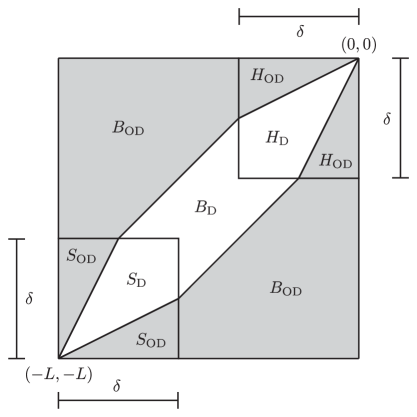
Figure 7. The square $[-L,0]^{2}$ in the $(\kappa,\lambda)$-plane is covered by the six regions $S_{\mathrm{D}}$, $S_{\mathrm{OD}}$, $B_{\mathrm{D}}$, $B_{\mathrm{OD}}$, $H_{D}$, and $H_{OD}$.

Here, the constant $\delta>0$ is as specified in Lemma 3.1. As $e(\kappa,\lambda)=e(\lambda,\kappa)$ it will be enough to show integrability of $e$ over the part of $[-L,0]^{2}$ with $\kappa<\lambda$, an inequality that we will assume tacitly below.

First we consider integrating $e(\kappa,\lambda)$ over the “off-diagonal” shaded regions $S_{\mathrm{OD}}$, $B_{\mathrm{OD}}$, and $H_{\mathrm{OD}}$ shown in Figure 7. An upper bound for $e(\kappa,\lambda)$ useful in these regions is easily obtained from the inequality $(a-b)^{2}\leq 2a^{2}+2b^{2}$:

(191) $$e(\kappa,\lambda)\leq 8\kappa F(\kappa)\lambda F(\lambda)\left[\frac{1}{(\kappa-\lambda)^{2}}+\frac{F(\kappa)F(\lambda)}{(m(\kappa)-m(\lambda))^{2}}\right],\quad(\kappa,\lambda)\in(-L,0)^{2}.$$

Applying the Mean Value Theorem to this estimate yields

(192) $$e(\kappa,\lambda)\leq\frac{8\kappa F(\kappa)\lambda F(\lambda)}{(\kappa-\lambda)^{2}}\left[1+\frac{F(\kappa)F(\lambda)}{F(\xi)^{2}}\right],$$

where $\kappa\leq\xi\leq\lambda$. Finally, since $F$ is monotone increasing according to Lemma 3.1 we obtain

(193) $$e(\kappa,\lambda)\leq\frac{8\kappa F(\kappa)\lambda F(\lambda)}{(\kappa-\lambda)^{2}}\left[1+\frac{F(\lambda)}{F(\kappa)}\right]=\frac{8\kappa F(\kappa)\lambda F(\lambda)}{(\kappa-\lambda)^{2}}+\frac{8\kappa\lambda F(\lambda)}{(\kappa-\lambda)^{2}}F(\lambda).$$

Now, for $(\kappa,\lambda)\in B_{\mathrm{OD}}$, we have that $\kappa-\lambda$ is bounded away from zero while by Lemma 3.1 $\kappa F(\kappa)$ and $\lambda F(\lambda)$ are bounded (and of course $|\kappa|<L$) while $F(\lambda)$ is integrable. Hence we easily conclude that $e(\kappa,\lambda)$ is integrable on $B_{\mathrm{OD}}$.

If $(\kappa,\lambda)\in H_{\mathrm{OD}}$ with $\kappa<\lambda$, then we have the inequality

(194) $$(\kappa-\lambda)^{2}=\left(\left[\lambda-\frac{\kappa}{2}\right]+\left[-\frac{\kappa}{2}\right]\right)^{2}\geq\frac{\kappa^{2}}{4},$$

and also since both $-\delta<\kappa<0$ and $-\delta<\lambda<0$ we may use the upper bound for $F$ given in (82) from Lemma 3.1 to replace (193) with

(195) $$e(\kappa,\lambda)\leq 32C_{0}^{2}(-\kappa)^{-1-1/q}(-\lambda)^{1-1/q}+32C_{0}^{2}(-\kappa)^{-1}(-\lambda)^{1-2/q},$$

where $C_{0}>0$ and $q>1$ are the constants in (82). This estimate is easily seen to be integrable on the component of $H_{\mathrm{OD}}$ with $\kappa<\lambda$ by direct calculation of the iterated integrals.

If $(\kappa,\lambda)\in S_{\mathrm{OD}}$ with $\kappa<\lambda$, then we have the inequality

(196) $$(\kappa-\lambda)^{2}=\left(\left[\frac{\lambda+L}{2}\right]+\left[\frac{\lambda+L}{2}-(\kappa+L)\right]\right)^{2}\geq\frac{(\lambda+L)^{2}}{4},$$

and also since both $-L<\kappa<-L+\delta$ and $-L<\lambda<-L+\delta$ we may use the upper bound for $F$ given in (80) from Lemma 3.1 along with the inequalities $|\kappa|<L$ and $|\lambda|<L$ to replace (193) with

(197) $$e(\kappa,\lambda)\leq 32L^{2}C_{-L}^{2}(\kappa+L)^{1/2}(\lambda+L)^{-3/2}+32L^{2}C_{-L}^{2}(\lambda+L)^{-1}.$$

This upper bound is obviously integrable on the component of $S_{\mathrm{OD}}$ with $\kappa<\lambda$.

Now we consider integrating $e(\kappa,\lambda)$ over the “diagonal” unshaded regions $S_{\mathrm{D}}$, $B_{\mathrm{D}}$, and $H_{\mathrm{D}}$ shown in Figure 7. By the Mean Value Theorem and the monotonicity of $F$ guaranteed by Lemma 3.1, we obtain an upper bound more useful when $\kappa\approx\lambda$:

(198) $$e(\kappa,\lambda)\leq 4\kappa F(\kappa)\lambda F(\lambda)\left[\frac{F(\kappa)-F(\lambda)}{m(\kappa)-m(\lambda)}\right]^{2},\quad(\kappa,\lambda)\in(-L,0)^{2}.$$

Again using the Mean Value Theorem and monotonicity of $F$ we may make the upper bound larger for $\kappa<\lambda$:

(199) $$e(\kappa,\lambda)\leq\frac{4\kappa\lambda F(\lambda)F^{\prime}(\xi)^{2}}{F(\kappa)},$$

where $\kappa\leq\xi\leq\lambda$.

For $(\kappa,\lambda)\in B_{\mathrm{D}}$ with $\kappa<\lambda$, both $\kappa$ and $\lambda$ are bounded away from the soft and hard edges of the eigenvalue spectrum, so Lemma 3.1 guarantees that $F$ and $F^{\prime}$ are bounded, and $F$ is also bounded away from zero by strict monotonicity and the boundary condition $F(-L)=0$. It follows from (199) that $e(\kappa,\lambda)$ is bounded and hence integrable on $B_{\mathrm{D}}$.

If $(\kappa,\lambda)\in H_{\mathrm{D}}$ then we may use the estimates (82) and (83) from Lemma 3.1 to replace (199) with

(200) $$e(\kappa,\lambda)\leq\frac{8C_{0}^{2}}{q^{2}}(-\kappa)^{1+1/q}(-\lambda)^{1-1/q}(-\xi)^{-2/q-2}\leq\frac{8C_{0}^{2}}{q^{2}}(-\kappa)^{1+1/q}(-\lambda)^{-1-3/q}.$$

The double integral of this upper bound over the region $H_{\mathrm{D}}$ with $\kappa<\lambda$ is easily computed by iterated integration and is clearly finite as a consequence of the fact that $q>1$.

Finally, if $(\kappa,\lambda)\in S_{\mathrm{D}}$ with $\kappa<\lambda$, then we may use the estimates (80) and (81) from Lemma 3.1 together with the inequalities $|\kappa|<L$ and $|\lambda|<L$ to replace (199) with

(201) $$e(\kappa,\lambda)\leq 2L^{2}C_{-L}^{2}(\kappa+L)^{-1/2}(\lambda+L)^{1/2}(\xi+L)^{-1}\leq 2L^{2}C_{-L}^{2}(\kappa+L)^{-3/2}(\lambda+L)^{1/2},$$

an upper bound that is clearly integrable over the part of $S_{\mathrm{D}}$ with $\kappa<\lambda$. ∎

Lemma 4.9.

The measure $\mu_{\epsilon}$ converges in the weak-$*$ sense to $\mu$, uniformly for $(x,t)$ in compact sets. That is, for each continuous function $f:\mathbb{R}\to\mathbb{C}$,

(202) $$\lim_{\epsilon\downarrow 0}\int_{\mathbb{R}}f(\alpha)\,d\mu_{\epsilon}(\alpha)=\int_{\mathbb{R}}f(\alpha)\,d\mu(\alpha),$$

with the limit being uniform with respect to $(x,t)$ in compact sets.

Proof.

According to Lemma 4.7, for each polynomial $p(\alpha)$ we have the following limit, uniform for $(x,t)$ in compact sets:

(203) $$\lim_{\epsilon\downarrow 0}\int_{\mathbb{R}}p(\alpha)\,d\mu_{\epsilon}(\alpha)=\int_{\mathbb{R}}p(\alpha)\,d\mu(\alpha).$$

But by Lemma 4.8 we can equivalently integrate over the compact interval $\Omega$ (independent of $(x,t)$ in any given compact set) with the same result. Now by the Weierstraß Approximation Theorem, given any continuous function $f:\mathbb{R}\to\mathbb{C}$ and any $\rho>0$ there is a polynomial $p^{f}_{\rho}(\alpha)$ for which

(204) $$\sup_{\lambda\in\Omega}|f(\alpha)-p^{f}_{\rho}(\alpha)|<\frac{\rho}{M},$$

so for any measure $\nu$ of mass $M$ with support in $\Omega$ (like $\mu_{\epsilon}$ and $\mu$),

(205) $$\left|\int_{\mathbb{R}}[f(\alpha)-p_{\rho}^{f}(\alpha)]\,d\nu(\alpha)\right|\leq\int_{\Omega}|f(\alpha)-p_{\rho}^{f}(\alpha)|\,d\nu(\alpha)<\rho.$$

Let $\omega>0$ be an arbitrarily small positive number. Then if we write

(206) $$\nu[g]:=\int_{\Omega}g(\alpha)\,d\nu(\alpha),$$

we have

(207) $$\begin{split}\left|\int_{\mathbb{R}}f(\alpha)\,d\mu_{\epsilon}(\alpha)-\int_{\mathbb{R}}f(\alpha)\,d\mu(\alpha)\right|&=\left|\mu_{\epsilon}[f]-\mu[f]\right|\\ &=\left|\left[\mu_{\epsilon}[p^{f}_{\omega/3}]-\mu[p^{f}_{\omega/3}]\right]+\mu_{\epsilon}[f-p^{f}_{\omega/3}]-\mu[f-p^{f}_{\omega/3}]\right|\\ &\leq\left|\mu_{\epsilon}[p^{f}_{\omega/3}]-\mu[p^{f}_{\omega/3}]\right|+\left|\mu_{\epsilon}[f-p^{f}_{\omega/3}]\right|+\left|\mu[f-p^{f}_{\omega/3}]\right|\\ &<\left|\mu_{\epsilon}[p^{f}_{\omega/3}]-\mu[p^{f}_{\omega/3}]\right|+\frac{2}{3}\omega,\end{split}$$

with the last inequality following from (205). But with $\omega>0$ fixed, (203) implies that $\epsilon>0$ may be chosen sufficiently small, independently of $(x,t)$ in any given compact set, that

(208) $$\left|\mu_{\epsilon}[p_{\omega/3}^{f}]-\mu[p_{\omega/3}^{f}]\right|<\frac{1}{3}\omega,$$

which implies

(209) $$\left|\int_{\mathbb{R}}f(\alpha)\,d\mu_{\epsilon}(\alpha)-\int_{\mathbb{R}}f(\alpha)\,d\mu(\alpha)\right|<\omega$$

thereby completing the proof. ∎

Now we are in a position to complete the proof of Proposition 4.2. We begin by writing $\tilde{U}_{\epsilon}(x,t)$ as defined by (93) in terms of the normalized (to mass $M$) counting measure $\mu_{\epsilon}$:

(210) $$\tilde{U}_{\epsilon}(x,t)=\left[\frac{\epsilon N(\epsilon)}{M}\right]\int_{\mathbb{R}}2\arctan(\epsilon^{-1}\alpha)\,d\mu_{\epsilon}(\alpha).$$

Define the continuous functions

(211) $$a_{+}(\alpha):=\pi+4H(-\alpha)\arctan(\alpha),\quad a_{-}(\alpha):=-a_{+}(-\alpha),\quad\alpha\in\mathbb{R},$$

where $H(\cdot)$ denotes the Heaviside step function. It is then easy to check (see Figure 8) that for any $E>0$,

Figure 8. The graphs of $a_{-}(\alpha)<a_{+}(\alpha)$ (black) and several graphs of $2\arctan(\epsilon^{-1}\alpha)$ for $\epsilon\leq 1$ (gray).

(212) $$0<\epsilon\leq E\quad\implies\quad a_{-}(E^{-1}\alpha)\leq 2\arctan(\epsilon^{-1}\alpha)\leq a_{+}(E^{-1}\alpha),\quad\alpha\in\mathbb{R}.$$

Therefore, for any $E>0$ and all $0<\epsilon<E$,

(213) $$\int_{\mathbb{R}}a_{-}(E^{-1}\alpha)\,d\mu_{\epsilon}(\alpha)\leq\int_{\mathbb{R}}2\arctan(\epsilon^{-1}\alpha)\,d\mu_{\epsilon}(\alpha)\leq\int_{\mathbb{R}}a_{+}(E^{-1}\alpha)\,d\mu_{\epsilon}(\alpha).$$

Using Lemma 4.9 we may pass to the limit $\epsilon\downarrow 0$ in the lower and upper bounds to obtain

(214) $$\liminf_{\epsilon\downarrow 0}\int_{\mathbb{R}}2\arctan(\epsilon^{-1}\alpha)\,d\mu_{\epsilon}(\alpha)\geq\int_{\mathbb{R}}a_{-}(E^{-1}\alpha)\,d\mu(\alpha)$$

and also

(215) $$\limsup_{\epsilon\downarrow 0}\int_{\mathbb{R}}2\arctan(\epsilon^{-1}\alpha)\,d\mu_{\epsilon}(\alpha)\leq\int_{\mathbb{R}}a_{+}(E^{-1}\alpha)\,d\mu(\alpha).$$

In these statements, $E>0$ is an arbitrary parameter, and the limits are uniform for $(x,t)$ in compact sets. But $a_{\pm}(E^{-1}\alpha)$ are uniformly bounded functions that both tend pointwise for $\alpha\neq 0$ to the same limit function $\pi\,\mathrm{sgn}(\lambda)$ as $E\downarrow 0$, while $\mu$ is a fixed measure that is absolutely continuous with respect to Lebesgue measure on $\mathbb{R}$, so by the Lebesgue Dominated Convergence Theorem,

(216) $$\lim_{E\downarrow 0}\int_{\mathbb{R}}a_{\pm}(E^{-1}\alpha)\,d\mu(\alpha)=\int_{\mathbb{R}}\pi\,\mathrm{sgn}(\alpha)\,d\mu(\alpha).$$

By letting $E\downarrow 0$, it then follows from (214) and (215) that

(217) $$\lim_{\epsilon\downarrow 0}\int_{\mathbb{R}}2\arctan(\epsilon^{-1}\alpha)\,d\mu_{\epsilon}(\alpha)=\int_{\mathbb{R}}\pi\,\mathrm{sgn}(\alpha)\,d\mu(\alpha)$$

with the limit being uniform for $(x,t)$ in any given compact set. Finally, according to (71), we have (independent of $x$ and $t$)

(218) $$\lim_{\epsilon\downarrow 0}\frac{\epsilon N(\epsilon)}{M}=1,$$

so combining this result with (217) and noting that $d\mu(\alpha)=G(\alpha;x,t)\,d\alpha$ completes the proof of Proposition 4.2.

4.4. Differentiation of $\tilde{U}_{\epsilon}$. Burgers’ equation and weak convergence of $\tilde{u}_{\epsilon}$

Let $\phi\in\mathscr{D}(\mathbb{R})$ be a test function. Then by integration by parts and the uniform convergence of $\tilde{U}_{\epsilon}(x,t)$ to $U(x,t)$ on compact sets in the $(x,t)$-plane guaranteed by Proposition 4.2,

(219) $$\begin{split}\lim_{\epsilon\downarrow 0}\int_{\mathbb{R}}\tilde{u}_{\epsilon}(x,t)\phi(x)\,dx&=\lim_{\epsilon\downarrow 0}\int_{\mathbb{R}}\frac{\partial\tilde{U}_{\epsilon}}{\partial x}(x,t)\phi(x)\,dx\\ &=-\lim_{\epsilon\downarrow 0}\int_{\mathbb{R}}\tilde{U}_{\epsilon}(x,t)\phi^{\prime}(x)\,dx\\ &=-\int_{\mathbb{R}}U(x,t)\phi^{\prime}(x)\,dx.\end{split}$$

Lemma 4.10.

The limit function $U(x,t)$ is continuously differentiable with respect to $x$, and if $(x,t)$ is a point for which there are $2P(x,t)+1$ solutions $u_{0}^{\mathrm{B}}(x,t)<\cdots<u_{2P(x,t)}^{\mathrm{B}}(x,t)$ of the implicit equation (224),

(220) $$\frac{\partial U}{\partial x}(x,t)=\sum_{n=0}^{2P(x,t)}(-1)^{n}u_{n}^{\mathrm{B}}(x,t),$$

and the above formula is extended to nongeneric $(x,t)$ by continuity.

Proof.

Exchanging the order of integration in the double-integral formula for $U(x,t)$ obtained by substituting $d\mu(\alpha)=G(\alpha;x,t)\,d\alpha$ with $G$ given by (100) into (99), we obtain

(221) $$U(x,t)=\int_{-L}^{0}J(\lambda;x,t)\,d\lambda,$$

where

(222) $$J(\lambda;x,t):=-\frac{1}{4\lambda}\int_{-2\lambda(x+2\lambda t-x_{+}(\lambda))}^{-2\lambda(x+2\lambda t-x_{-}(\lambda))}\mathrm{sgn}(\alpha)\,d\alpha.$$

Note that for $\lambda\in[-L,0]$ the upper limit of integration is greater than or equal to the lower limit. Moreover the integral in $J(\lambda;x,t)$ is easily evaluated; for $-L<\lambda<0$,

(223) $$J(\lambda;x,t)=\begin{cases}-\pi F(\lambda),\quad&x+2\lambda t-x_{-}(\lambda)<0,\\ x+2\lambda t+\gamma(\lambda),\quad&x+2\lambda t-x_{+}(\lambda)\leq 0\leq x+2\lambda t-x_{-}(\lambda)\\ \pi F(\lambda),\quad&x+2\lambda t-x_{+}(\lambda)>0.\end{cases}$$

It follows from the relations $x_{\pm}(\lambda)=\pm\pi F(\lambda)-\gamma(\lambda)$ that for an admissible initial condition $u_{0}$, $J$ is a continuous function of $x$ for each fixed $t$, uniformly with respect to $\lambda\in[-L,0]$, and hence also from (221) that $U(\cdot,t)$ is continuous on $\mathbb{R}$ for each $t$. To prove that $U(\cdot,t)$ is continuously differentiable it will therefore suffice to establish continuous differentiability on the complement of a finite set of points and that the resulting piecewise formula for $\partial U/\partial x$ extends continuously to the whole real line.

To use the formula (223) in the representation (221) we therefore need to know those points $\lambda\in(-L,0)$ at which one of the two quantities $x+2\lambda t-x_{+}(\lambda)<x+2\lambda t-x_{-}(\lambda)$ changes sign. Under the variable substitution $\lambda=-u^{\mathrm{B}}$, the definition of the turning points $x_{\pm}(\lambda)$ as branches of the inverse function of $u_{0}$ implies that the union of solutions of the two equations $x+2\lambda t-x_{\pm}(\lambda)=0$ is exactly the totality of solutions of the implicit equation

(224) $$u^{\mathrm{B}}=u_{0}(x-2u^{\mathrm{B}}t).$$

In other words, the transitional points $\lambda$ for the formula (223) correspond under the sign change $u^{\mathrm{B}}=-\lambda$ to the branches of the multivalued solution of Burgers’ equation

(225) $$\frac{\partial u^{\mathrm{B}}}{\partial t}+2u^{\mathrm{B}}\frac{\partial u^{\mathrm{B}}}{\partial x}=0$$

subject to the admissible initial condition $u^{\mathrm{B}}(x,0)=u_{0}(x)$.

Note that admissibility of $u_{0}$ implies (see Definition 3.1) that given any $t\in\mathbb{R}$ there exist only a finite number of breaking points $(x_{\xi},t_{\xi})$ with $t_{\xi}$ in the closed interval between $0$ and $t$. Indeed, the breaking points correspond to values of $\xi\in\mathbb{R}$ for which $u_{0}^{\prime\prime}(\xi)=0$ but $u_{0}^{\prime\prime\prime}(\xi)\neq 0$, and the breaking times are $t_{\xi}=(-2u_{0}^{\prime}(\xi))^{-1}$; since $u_{0}^{\prime}(\xi)$ decays to zero for large $\xi$, bounded breaking times $t_{\xi}$ correspond to bounded $\xi$, and there are only finitely many of these by hypothesis. Moreover, each breaking point $(x_{\xi},t_{\xi})$ generates a new fold in the solution surface lying between two caustic curves emerging in the direction of increasing $|t|$ from $(x_{\xi},t_{\xi})$, and because $u^{\prime\prime\prime}(\xi)\neq 0$ there are exactly two more sheets of the multivalued solution of Burgers’ equation born within the fold as a result of a simple pitchfork bifurcation. Therefore, the union of caustic curves and breaking points meets any line of constant $t$ in the $(x,t)$-plane in a finite set of points $\{x_{j}^{\mathrm{crit}}(t)\}$, and on every connected component of the set $S_{t}:=\{(x,t)|x\in\mathbb{R}\setminus\{x_{j}^{\mathrm{crit}}(t)\}\}$, there is a finite, odd, and constant (with respect to $x$) number $2P(x,t)+1$ of roots of the equation (224), and all roots are simple (and hence differentiable with respect to $x$).

If $t\geq 0$, then by admissibility of $u_{0}$ the quantity $b_{-}(\lambda;x,t):=x+2\lambda t-x_{-}(\lambda)$ is strictly increasing as a function of $\lambda$ on the interval $(-L,0)$, and therefore in this interval there can exist at most one root of $b_{-}(\lambda;x,t)$, regardless of the value of $x\in\mathbb{R}$. Moreover, $b_{-}(\lambda;x,t)\to+\infty$ as $\lambda\uparrow 0$, so there will be exactly one root in $(-L,0)$ if $b_{-}(-L;x,t)=x-x_{0}-2Lt<0$ and no root in $(-L,0)$ if $x-x_{0}-2Lt>0$. Since $b_{+}(\lambda;x,t):=x+2\lambda t-x_{+}(\lambda)<b_{-}(\lambda;x,t)$ for $-L<\lambda<0$, if $x-x_{0}-2Lt<0$, all roots of $b_{+}(\lambda;x,t)$ in $(-L,0)$ must lie to the right of the root of $b_{-}(\lambda;x,t)$. Thus, for $x\in S_{t}\setminus\{x_{0}+2Lt\}$, we either have

(226) $$\begin{split}U(x,t)&=\int_{-u_{0}^{\mathrm{B}}}^{0}(x+2\lambda t+\gamma(\lambda))\,d\lambda\\ &\quad\quad\quad{}+\sum_{p=1}^{P(x,t)}\left[\pi\int_{-u_{2p-1}^{\mathrm{B}}}^{-u_{2p-2}^{\mathrm{B}}}F(\lambda)\,d\lambda+\int_{-u_{2p}^{\mathrm{B}}}^{-u_{2p-1}^{\mathrm{B}}}(x+2\lambda t+\gamma(\lambda))\,d\lambda\right]\\ &\quad\quad\quad\quad\quad{}+\pi\int_{-L}^{-u_{2P(x,t)}^{\mathrm{B}}}F(\lambda)\,d\lambda,\quad x\in S_{t},\quad x>x_{0}+2Lt,\end{split}$$

in which case $u_{0}^{\mathrm{B}}(x,t)<\cdots<u_{2P(x,t)}^{\mathrm{B}}(x,t)$ are all roots of $b_{+}(-u^{\mathrm{B}};x,t)$, or

(227) $$\begin{split}U(x,t)&=\int_{-u_{0}^{\mathrm{B}}}^{0}(x+2\lambda t+\gamma(\lambda))\,d\lambda\\ &\quad\quad\quad{}+\sum_{p=1}^{P(x,t)}\left[\pi\int_{-u_{2p-1}^{\mathrm{B}}}^{-u_{2p-2}^{\mathrm{B}}}F(\lambda)\,d\lambda+\int_{-u_{2p}^{\mathrm{B}}}^{-u_{2p-1}^{\mathrm{B}}}(x+2\lambda t+\gamma(\lambda))\,d\lambda\right]\\ &\quad\quad\quad\quad\quad{}-\pi\int_{-L}^{-u_{2P(x,t)}^{\mathrm{B}}}F(\lambda)\,d\lambda,\quad x\in S_{t},\quad x<x_{0}+2Lt,\end{split}$$

in which case $u_{0}^{\mathrm{B}}(x,t)<\cdots<u_{2P(x,t)-1}^{\mathrm{B}}(x,t)$ are roots of $b_{+}(-u^{\mathrm{B}};x,t)$ while $u_{2P(x,t)}^{\mathrm{B}}(x,t)$ with $u_{2P(x,t)}^{\mathrm{B}}(x,t)>u_{2P(x,t)-1}^{\mathrm{B}}(x,t)$ is a root of $b_{-}(-u^{\mathrm{B}};x,t)$. In both cases, the condition $x\in S_{t}$ guarantees that all roots are differentiable with respect to $x$, so we may calculate $\partial U/\partial x$ by Leibniz’ rule:

(228) $$\begin{split}\frac{\partial U}{\partial x}(x,t)&=b_{+}(-u_{2P}^{\mathrm{B}}(x,t);x,t)\frac{\partial u_{2P}^{\mathrm{B}}}{\partial x}(x,t)+\sum_{n=0}^{2P-1}(-1)^{n}b_{+}(-u_{n}^{\mathrm{B}}(x,t);x,t)\frac{\partial u_{n}^{\mathrm{B}}}{\partial x}(x,t)\\ &\quad\quad{}+\sum_{n=0}^{2P}(-1)^{n}u_{n}^{\mathrm{B}}(x,t),\quad x\in S_{t},\quad x>x_{0}+2Lt,\end{split}$$

or

(229) $$\begin{split}\frac{\partial U}{\partial x}(x,t)&=b_{-}(-u_{2P}^{\mathrm{B}}(x,t);x,t)\frac{\partial u_{2P}^{\mathrm{B}}}{\partial x}(x,t)+\sum_{n=0}^{2P-1}(-1)^{n}b_{+}(-u_{n}^{\mathrm{B}}(x,t);x,t)\frac{\partial u_{n}^{\mathrm{B}}}{\partial x}(x,t)\\ &\quad\quad{}+\sum_{n=0}^{2P}(-1)^{n}u_{n}^{\mathrm{B}}(x,t),\quad x\in S_{t},\quad x<x_{0}+2Lt,\end{split}$$

where in both cases $P=P(x,t)$ is a constant nonnegative integer on each connected component of $S_{t}$. The terms on the first line in each of these formulae arise from differentiating the limits of integration and using $x_{\pm}(\lambda)=\pm\pi F(\lambda)-\gamma(\lambda)$, while the terms on the second line arise from the explicit partial differentiation of the integrand $x+2\lambda t+\gamma(\lambda)$ with respect to $x$. It follows from our division of the solutions of (224) among the roots of $b_{+}$ and $b_{-}$ that in both cases the terms on the first line vanish identically, with the result that

(230) $$\frac{\partial U}{\partial x}(x,t)=\sum_{n=0}^{2P(x,t)}(-1)^{n}u_{n}^{\mathrm{B}}(x,t),\quad x\in S_{t}\setminus\{x_{0}+2Lt\}.$$

This expression is clearly continuous in $x$ on each connected component of $S_{t}\setminus\{x_{0}+2Lt\}$. Moreover, it extends continuously to the finite complement in $\mathbb{R}_{x}$ (at fixed $t\geq 0$) because at caustics pairs of solution branches entering into (230) with opposite signs simply coalesce. Therefore $U(\cdot,t)$ is indeed continuously differentiable for $t\geq 0$ and its derivative is given by the desired simple formula (220). Virtually the same argument applies to $t\leq 0$ with the roles of $b_{\pm}(\lambda;x,t)$ reversed, and the resulting formula for $\partial U/\partial x$ is the same. ∎

It follows from this result that we may integrate by parts in (219) and obtain

(231) $$\lim_{\epsilon\downarrow 0}\int_{\mathbb{R}}\tilde{u}_{\epsilon}(x,t)\phi(x)\,dx=\int_{\mathbb{R}}\frac{\partial U}{\partial x}(x,t)\phi(x)\,dx$$

for every test function $\phi\in\mathscr{D}(\mathbb{R})$. Now let $v\in L^{2}(\mathbb{R})$. Since $\mathscr{D}(\mathbb{R})$ is dense in $L^{2}(\mathbb{R})$, for each $\sigma>0$ there exists a test function $\phi_{\sigma}\in\mathscr{D}(\mathbb{R})$ such that

(232) $$\|\phi_{\sigma}-v\|_{2}^{2}:=\int_{\mathbb{R}}|\phi_{\sigma}(x)-v(x)|^{2}\,dx<\sigma^{2}.$$

Then,

(233) $$\begin{split}\int_{\mathbb{R}}\left[\tilde{u}_{\epsilon}(x,t)-\frac{\partial U}{\partial x}(x,t)\right]v(x)\,dx&=\int_{\mathbb{R}}\left[\tilde{u}_{\epsilon}(x,t)-\frac{\partial U}{\partial x}(x,t)\right]\phi_{\sigma}(x)\,dx\\ &\quad\quad{}+\int_{\mathbb{R}}\frac{\partial U}{\partial x}(x,t)\left[\phi_{\sigma}(x)-v(x)\right]\,dx\\ &\quad\quad{}-\int_{\mathbb{R}}\tilde{u}_{\epsilon}(x,t)\left[\phi_{\sigma}(x)-v(x)\right]\,dx.\end{split}$$

Observe that, according to the definition (see Definition 3.2) of $\tilde{u}_{\epsilon}(x,t)$ in terms of the modified scattering data, it follows from (47) and (46) that

(234) $$\int_{\mathbb{R}}\tilde{u}_{\epsilon}(x,t)^{2}\,dx=-4\pi\epsilon\sum_{n=1}^{N(\epsilon)}\tilde{\lambda}_{n}.$$

This Riemann sum converges as $\epsilon\downarrow 0$:

(235) $$\lim_{\epsilon\downarrow 0}\int_{\mathbb{R}}\tilde{u}_{\epsilon}(x,t)^{2}\,dx=-4\pi\int_{-L}^{0}\lambda F(\lambda)\,d\lambda=\int_{\mathbb{R}}u_{0}(x)^{2}\,dx,$$

where the second equality follows from the identities (57), which essentially define $F(\lambda)$ in terms of the admissible initial condition $u_{0}$. Therefore, $\|\tilde{u}_{\epsilon}(\cdot,t)\|_{2}$ is bounded for sufficiently small $\epsilon$, independently of $t$.

Also, $\partial U/\partial x$ is independent of $\epsilon$ and from the formula (220) it is easy to check that it is positive and bounded above by the constant $L$ for all $(x,t)$. Therefore

(236) $$\left\|\frac{\partial U}{\partial x}(\cdot,t)\right\|_{2}^{2}\leq L\int_{\mathbb{R}}\frac{\partial U}{\partial x}(x,t)\,dx.$$

By the formula (220), the latter integral is equal to the area between the graph of the multivalued solution curve for Burgers’ equation and the $x$-axis. Since points on the graph at the same height move with the same speed, this area is independent of time $t$, and hence we have

(237) $$\left\|\frac{\partial U}{\partial x}(\cdot,t)\right\|_{2}^{2}\leq 2\pi LM,$$

where the mass $M$ is defined in terms of the initial condition $u_{0}$ by (52). In fact, for $0\leq t<T$, where $T$ is the breaking time, it follows from the fact that $\partial U/\partial x$ as given by (220) reduces to the classical solution $u_{0}^{\mathrm{B}}(x,t)$ of Burgers’ equation with initial data $u_{0}$, which conserves exactly the $L^{2}(\mathbb{R}_{x})$ norm, that

(238) $$\left\|\frac{\partial U}{\partial x}(\cdot,t)\right\|^{2}_{2}=\|u_{0}^{B}(\cdot,t)\|^{2}_{2}=\int_{\mathbb{R}}u_{0}(x)^{2}\,dx,\quad 0\leq t<T.$$

We will use this fact below in §5 when we prove Corollary 1.1. In any case, these considerations show that for all $\epsilon>0$ sufficiently small there exists a constant $K>0$ independent of $t$ such that

(239) $$\left\|\frac{\partial U}{\partial x}(\cdot,t)\right\|_{2}+\|\tilde{u}_{\epsilon}(\cdot,t)\|_{2}\leq K$$

holds for all $t\geq 0$.

Now, by Cauchy-Schwarz it follows that

(240) $$\left|\int_{\mathbb{R}}\frac{\partial U}{\partial x}(x,t)\left[\phi_{\sigma}(x)-v(x)\right]\,dx-\int_{\mathbb{R}}\tilde{u}_{\epsilon}(x,t)\left[\phi_{\sigma}(x)-v(x)\right]\,dx\right|\leq K\|\phi_{\sigma}-v\|_{2}.$$

Given $\omega>0$ arbitrarily small, we then choose $\sigma=\omega/(2M)$ and then (233) implies that

(241) $$\left|\int_{\mathbb{R}}\left[\tilde{u}_{\epsilon}(x,t)-\frac{\partial U}{\partial x}(x,t)\right]v(x)\,dx\right|\leq\left|\int_{\mathbb{R}}\left[\tilde{u}_{\epsilon}(x,t)-\frac{\partial U}{\partial x}(x,t)\right]\phi_{\omega/(2M)}(x)\,dx\right|+\frac{\omega}{2}.$$

Finally, since $\phi_{\omega/(2M)}$ is a test function independent of $\epsilon$, we may use (231) to choose $\epsilon>0$ so small that the first term on the right-hand side is less than $\omega/2$.

This proves that

(242) $$\mathop{\mathrm{w}_{x}\mathrm{-lim}}_{\epsilon\downarrow 0}\tilde{u}_{\epsilon}(x,t)=\frac{\partial U}{\partial x}(x,t)$$

(weak $L^{2}$ convergence) uniformly for $t$ in bounded intervals. Combining (220) with (242) completes the proof of Theorem 1.1.

5. Strong Convergence Before Breaking

In this brief section we give a proof of Corollary 1.1, following closely Lax and Levermore (see Theorem 4.5 in part II of [20]). Starting from the identity

(243) $$\|\tilde{u}_{\epsilon}(\cdot,t)-u_{0}^{\mathrm{B}}(\cdot,t)\|_{2}^{2}=\int_{\mathbb{R}}\tilde{u}_{\epsilon}(x,t)^{2}\,dx+\int_{\mathbb{R}}u_{0}^{\mathrm{B}}(x,t)^{2}\,dx-2\int_{\mathbb{R}}\tilde{u}_{\epsilon}(x,t)u_{0}^{\mathrm{B}}(x,t)\,dx,$$

we note that for $0\leq t<T$, where $T$ is the breaking time, (235) and (238) imply that

(244) $$\lim_{\epsilon\downarrow 0}\|\tilde{u}_{\epsilon}(\cdot,t)-u_{0}^{\mathrm{B}}(\cdot,t)\|_{2}^{2}=2\int_{\mathbb{R}}u_{0}(x)^{2}\,dx-2\lim_{\epsilon\downarrow 0}\int_{\mathbb{R}}\tilde{u}_{\epsilon}(x,t)u_{0}^{\mathrm{B}}(x,t)\,dx.$$

But $u_{0}^{\mathrm{B}}(\cdot,t)\in L^{2}(\mathbb{R})$ is independent of $\epsilon$, so by Theorem 1.1,

(245) $$\lim_{\epsilon\downarrow 0}\int_{\mathbb{R}}\tilde{u}_{\epsilon}(x,t)u_{0}^{\mathrm{B}}(x,t)\,dx=\int_{\mathbb{R}}u_{0}^{\mathrm{B}}(x,t)^{2}\,dx=\int_{\mathbb{R}}u_{0}(x)^{2}\,dx,$$

with the second equality following from (238) for $0\leq t<T$. Therefore

(246) $$\lim_{\epsilon\downarrow 0}\|\tilde{u}_{\epsilon}(\cdot,t)-u_{0}^{\mathrm{B}}(\cdot,t)\|_{2}=0$$

as desired, and the proof is complete.

6. Numerical Verification

To illustrate the weak convergence of $\tilde{u}_{\epsilon}(x,t)$ as guaranteed by Theorem 1.1, and to attempt to empirically quantify the rate of convergence, we have directly used the exact formula (93) for $\tilde{U}_{\epsilon}(x,t)$ having first chosen the modified scattering data corresponding to the admissible initial condition $u_{0}(x)=2(1+x^{2})^{-1}$ as specified in Definition 3.2, and compared the result for several different values of $\epsilon$ with the limiting formula (99) for $U(x,t)$. Our results are shown in Figure 9.

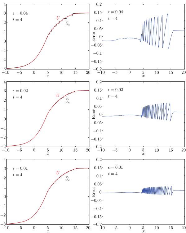
Figure 9. Left: plots of $\tilde{U}_{\epsilon}(x,t)$ (black) and its locally uniform limit $U(x,t)$ (red) at $t=4$ for various values of $\epsilon$. For these plots, $u_{0}(x):=2(1+x^{2})^{-1}$. Right: corresponding plots of the error $U(x,t)-\tilde{U}_{\epsilon}(x,t)$.

These plots clearly display the locally uniform convergence specified in Proposition 4.2. An interesting feature is the apparent regular “staircase” form of the graph of $\tilde{U}_{\epsilon}(x,t)$ as a function of $x$; that the steps have nearly equal height is a consequence of the fact that near the leading edge of the oscillation zone for $u_{\epsilon}$ (which lies approximately in the range $4<x<16$ in these plots) the undular bore wavetrain that is generated from the smooth initial data resolves into a train of solitons of the BO equation, each of which has a fixed mass proportional to $\epsilon$ (independent of amplitude and velocity).

To the eye, the size of the error between $\tilde{U}_{\epsilon}(x,t)$ and $U(x,t)$ appears to scale with $\epsilon$. To confirm this more quantitatively, we collected numerical data from several experiments, each performed with a different value of $\epsilon$ at the fixed time $t=4$. The supremum norm, calculated over the interval $-10<x<20$, of the error resulting from each of these experiments is plotted in Figure 10.

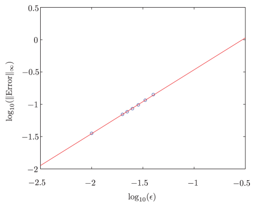
Figure 10. Circles: $\log_{10}(\|\tilde{U}_{\epsilon}(\cdot,4)-U(\cdot,4)\|_{\infty})$ for $\epsilon=1/25$, $1/30$, $1/35$, $1/40$, $1/45$, $1/50$, and $1/100$, as a function of $\log_{10}(\epsilon)$. In red: The least-squares linear fit.

On this plot with logarithmic axes, the data points appear to lie along a straight line, and we calculated the least squares linear fit to the data to be given by

(247) $$\log_{10}(\|\tilde{U}_{\epsilon}(\cdot,4)-U(\cdot,4)\|_{\infty})=0.988\log_{10}(\epsilon)+0.523$$

where the slope and intercept are given to three significant digits. This strongly suggests a linear rate of convergence, in which the error is asymptotically proportional to $\epsilon$ as $\epsilon\downarrow 0$.

The initial data $u_{0}(x)=2(1+x^{2})^{-1}$ was chosen for these experiments because it is the only initial condition (up to a constant multiple) for which the exact scattering data is known for a sequence of values of $\epsilon$ tending to zero. This is the result of a calculation of Kodama, Ablowitz, and Satsuma [18], who showed that if $u_{0}(x)=2(1+x^{2})^{-1}$, then the reflection coefficient $\beta(\lambda)$ vanishes identically if $\epsilon=1/N$ for any positive integer $N$. Moreover, there are in this case exactly $N$ eigenvalues $\lambda_{1}<\lambda_{2}<\cdots<\lambda_{N}$ of the operator $\mathcal{L}$ defined by (6), and they are given implicitly by the equation

(248) $$L_{N}\left(-\frac{2\lambda_{n}}{\epsilon}\right)=L_{N}\left(-2N\lambda_{n}\right)=0,$$

where $L_{N}$ is the Laguerre polynomial of degree $N$. The corresponding phase constants $\gamma_{n}$ all vanish exactly. The approximate eigenvalues determined from the initial condition $u_{0}$ via the formula (72) do not agree exactly with the scaled roots of the Laguerre polynomial of degree $N$ (although the approximate phase constants agree exactly with the true phase constants), so it is a worthwhile exercise to compare the function $\tilde{u}_{\epsilon}(x,t)$ as specified by Definition 3.2 with the true solution $u_{\epsilon}(x,t)$ of the Cauchy problem for the BO equation with initial data $u_{0}(x)=2(1+x^{2})^{-1}$. Of course Corollary 1.1 guarantees strong convergence in $L^{2}$ at $t=0$ (that is, $\tilde{u}_{\epsilon}(\cdot,0)$ is $L^{2}$-close to $u_{0}(\cdot)$) but this alone does not guarantee that $\tilde{u}_{\epsilon}(x,t)$ approximates $u_{\epsilon}(x,t)$ in any sense for $t>0$. We made the comparison for several values of $\epsilon>0$ corresponding to a reflectionless exact solution of the Cauchy problem constructed from the determinantal formula (39) at the time $t=4$, which is well beyond the breaking time. Our results are shown in Figure 11.

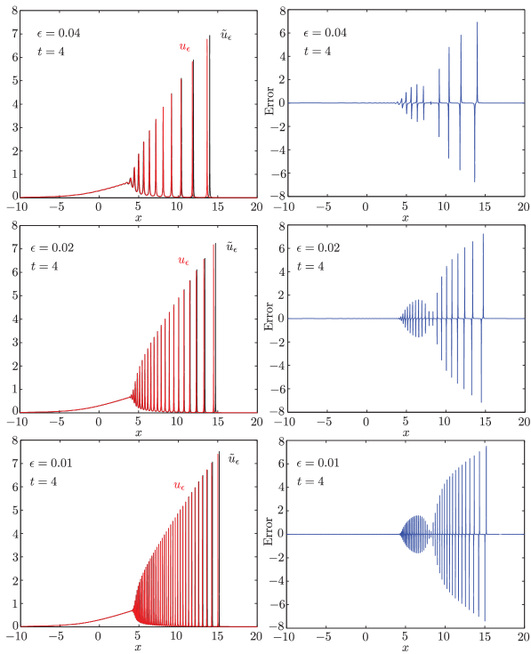
Figure 11. Left: plots of $\tilde{u}_{\epsilon}(x,t)$ (black) shown together with $u_{\epsilon}(x,t)$ (red) for the initial data $u_{0}(x)=2(1+x^{2})^{-1}$ shown for several values of $\epsilon$ at $t=4$. Right: The error $u_{\epsilon}(x,t)-\tilde{u}_{\epsilon}(x,t)$.

These plots show that the modification of the scattering data used to construct $\tilde{u}_{\epsilon}(x,t)$ results in a phase shift relative to $u_{\epsilon}(x,t)$ that is proportional to $\epsilon$, the approximate wavelength of the oscillations in the undular bore structure. In particular, $\tilde{u}_{\epsilon}(x,t)$ does not remain close to $u_{\epsilon}(x,t)$ after the breaking time in any strong sense, although is appears highly likely that convergence is restored in the weak topology.

7. Conclusion

In this paper, we have obtained the first rigorous results regarding the zero-dispersion limit of the Cauchy problem for the BO equation. As suggested by the formal mulitphase averaging of modulated $N$-phase wavetrain solutions carried out by Dobrokhotov and Krichever [9], the scalar inviscid Burgers’ equation and its multivalued solution after wave breaking characterizes the limit.

To analyze the BO Cauchy problem, we used a remarkable formula of Matsuno [22, 23] for the density of eigenvalues of the nonlocal operator $\mathcal{L}$ appearing in the scattering theory, and we have proposed a new asymptotic formula (68) for the corresponding phase constants necessary to set up the inverse-scattering problem. We then developed an analogue of the Lax-Levermore method [20] to study the inverse-scattering problem, and we obtained an explicit formula (100) for a measure $\mu$ with density $G(\alpha;x,t)$ that is the BO equivalent of the extremal measure in Lax-Levermore theory. By contrast with the KdV case, the formula we obtain for the weak limit from this measure is remarkably simple and explicit, writing the weak limit as a signed sum of branches of the multivalued solution of Burgers’ equation.

A useful generalization of the weak limit given in this paper is to consider the weak limits of all of the variational derivatives

(249) $$K_{n}:=\frac{\delta I_{n}}{\delta u},\quad n=3,4,5,\dots,$$

where the $I_{n}$ is the $n^{\mathrm{th}}$ conserved quantity given by (45). Each of the quantities $K_{n}$ can be written in the form

(250) $$K_{n+2}=\frac{\partial}{\partial t_{n}}\tilde{U}_{\epsilon}(x,t_{1},t_{2},\dots,t_{n})$$

where after the differentiation $t_{1}$ is set equal to $t$ and all $t_{k}$ for $k>1$ are set to zero. Here $\tilde{U}_{\epsilon}(x,t_{1},t_{2},\dots,t_{n})$ is given by (93) with each occurrence of $2t$ in the expression $-2\tilde{\lambda}_{k}(x+2\tilde{\lambda}_{k}t)$ occurring in the matrix elements of $\tilde{\mathbf{A}}_{\epsilon}$ replaced by $2t_{1}-3\tilde{\lambda}_{k}t_{2}+4\tilde{\lambda}_{k}^{2}t_{3}-5\tilde{\lambda}_{k}^{3}t_{4}+\cdots+(-1)^{n+1}(n+1)\tilde{\lambda}_{k}^{n-1}t_{n}$. Formulas for these higher weak limits can also be obtained within the framework of our method and will be published in a subsequent paper.

We are also currently investigating prospects for strengthening the limit after wave breaking occurs. The goal here is to rigorously establish an asymptotic formula for $\tilde{u}_{\epsilon}(x,t)$ that is valid pointwise for $(x,t)$ in the oscillation zone. Such a formula should accurately resolve the microscopic (wavelength proportional to $\epsilon$) oscillations, including finding the phase up to error terms that are bounded by a vanishingly small fraction of the wavelength. One expects the asymptotic form of the wavetrain to be given by the rational-exponential formulae found by Dobrokhotov and Krichever [9]. For the KdV equation such pointwise asymptotics have been obtained [8] using the Deift-Zhou steepest descent technique for matrix-valued Riemann-Hilbert problems. We are working to extend this kind of methodology to the context of scalar Riemann-Hilbert problems with nonlocal jump conditions, as occurs in the inverse-scattering transform (generally with nonvanishing reflection coefficient) for the BO equation.

It has been recently conjectured by Dubrovin [10] that near the earliest breaking point $(x_{\xi},t_{\xi})$ the solution of the Cauchy problem for quite general weakly dispersive Hamiltonian perturbations of Burgers’ equation should exhibit a universal form expressed in terms of Painlevé transcendents. This conjecture has been confirmed for general initial data for the KdV equation (as a particular case of a perturbation considered by Dubrovin) by Claeys and Grava [5]. It would be interesting to determine by direct calculation of the solution near the breaking point $(x_{\xi},t_{\xi})$ whether the BO equation should be considered to fall within the universality class of equations conjectured by Dubrovin.

8. Acknowledgements

This work was supported by the National Science Foundation under grant number DMS-0807653.

References

- [1] M. J. Ablowitz, A. S. Fokas and R. L. Anderson, “The direct linearizing transform and the Benjamin-Ono equation,” Phys. Lett. A 93, 375–378 (1983).
- [2] T. B. Benjamin, “Internal waves of permanent form in fluids of great depth,” J. Fluid Mech. 29, 559–592 (1967).
- [3] T. L. Bock and M. D. Kruskal, “A two-parameter Miura transformation of the Benjamin-Ono equation,” Phys. Lett. 74A, 173–176 (1979).
- [4] W. Choi and R. Camassa, “Weakly nonlinear internal waves in a two-fluid system,” J. Fluid. Mech. 313, 83–103 (1996).
- [5] T. Claeys and T. Grava, “Universality of the break-up profile for the KdV equation in the small dispersion limit using the Riemann-Hilbert approach,” Comm. Math. Phys. 286, 979–1009 (2009).
- [6] R. R. Coifman and M. V. Wickerhauser, “The scattering transform for the Benjamin-Ono equation,” Inverse Prob. 6, 825–861 (1990).
- [7] R. E. Davis and A. Acrivos, “Solitary internal waves in deep water,” J. Fluid Mech. 29, 593–607 (1967).
- [8] P. Deift, S. Venakides and X. Zhou, “New results in small dispersion KdV by an extension of the steepest descent method for Riemann-Hilbert problems,” Internat. Math. Research Not. 6, 286-299 (1997).
- [9] S. Yu. Dobrokhotov and I. M. Krichever, “Multi-phase solutions of the Benjamin-Ono equation and their averaging,” Mat. Zametki 49, 42–58 (1991).
- [10] B. A. Dubrovin, “On universality of critical behaviour in Hamiltonian PDEs,” Geometry, topology, and mathematical physics, Amer. Math. Soc. Transl. Ser. 2, 224, 59–109, Amer. Math. Soc., Providence, RI (2008).
- [11] B. A. Dubrovin, V. B. Matveev and S. P. Novikov, “Non-linear equations of Korteweg-de Vries type, finite-zone operators, and Abelian varieties,” Russian Math. Surveys 31, 59–146 (1976).
- [12] H. Flaschka, M. G. Forest and D. W. McLaughlin, “Multiphase averaging and the inverse spectral solution of the Korteweg-de Vries equation,” Comm. Pure Appl. Math. 33, 739–784 (1980).
- [13] A. S. Fokas and M. J. Ablowitz, “The inverse scattering transform for the Benjamin-Ono equation: a pivot to multidimensional problems,” Stud. Appl. Math. 68, 1–10 (1983).
- [14] A. V. Gurevich and L. P. Pitaevskii, “Nonstationary structure of a collisionless shock wave,” Soviet Phys. JETP 38, 291–297 (1974).
- [15] A. R. Its and V. B. Matveev, “Hill operators with a finite number of lacunae,” Functional Anal. Appl. 9, 65–66 (1975).
- [16] M. C. Jorge, A. A. Minzoni and N. F. Smyth, “Modulation solutions for the Benjamin-Ono equation,” Physica D 132, 1–18 (1999).
- [17] D. J. Kaup and Y. Matsuno, “The inverse scattering transform for the Benjamin-Ono equation,” Stud. Appl. Math. 101, 73–98 (1998).
- [18] Y. Kodama, M. J. Ablowitz and J. Satsuma, “Direct and inverse scattering problems of the nonlinear intermediate long wave equation,” J. Math. Phys. 23, 564–576 (1982).
- [19] P. D. Lax, “On dispersive difference schemes,” Physica 18D, 250–254 (1986).
- [20] P. D. Lax and C. D. Levermore, “The small dispersion limit of the Korteweg-de Vries equation,” Comm. Pure Appl. Math. 36, 253–290, 571–593, and 809–929 (three parts) (1983).
- [21] Y. Matsuno, “Exact multi-soliton solution of the Benjamin-Ono equation,” J. Phys. A Math. Gen. 12, 619–621 (1979).
- [22] Y. Matsuno, “Number density function of Benjamin-Ono solitons,” Phys. Lett. A 87, 15–17 (1981).
- [23] Y. Matsuno, “Asymptotic properties of the Benjamin-Ono equation,” J. Phys. Soc. Jpn. 51, 667–674 (1982).
- [24] Y. Matsuno, “Nonlinear modulation of periodic waves in the small dispersion limit of the Benjamin-Ono equation,” Phys. Rev. E 58, 7934–7940 (1998).
- [25] Y. Matsuno, “The small dispersion limit of the Benjamin-Ono equation and the evolution of a step initial condition,” J. Phys. Soc. Jpn. 67, 1814–1817 (1998).
- [26] P. D. Miller, Applied Asymptotic Analysis, Graduate Studies in Mathematics 75, American Mathematical Society, Providence, 2006.
- [27] A. Nakamura, “Bäcklund transform and conservation laws of the Benjamin-Ono equation,” J. Phys. Soc. Jpn. 47, 1335–1340 (1979).
- [28] A. Porter and N. F. Smyth, “Modelling the morning glory of the Gulf of Carpentaria,” J. Fluid Mech. 454, 1–20 (2002).
- [29] H. Ono, “Algebraic solitary waves in stratified fluids,” J. Phys. Soc. Jpn. 39, 1082–1091 (1975).
- [30] S. Venakides, “The Korteweg-de Vries equation with small dispersion: higher order Lax-Levermore theory,” Comm. Pure Appl. Math. 43, 335–361 (1990).
- [31] G. B. Whitham, “Non-linear dispersive waves,” Proc. Roy. Soc. Ser. A 283, 238–261 (1965).
- [32] E. Wigner, “Characteristic vectors of bordered matrices with infinite dimensions,” Ann. of Math. 62, 548–564 (1955).
- [33] E. Wigner, “On the distribution of the roots of certain symmetric matrices,” Ann. of Math. 67, 325–328 (1958).