Streams and caustics: the fine-grained structure of $\Lambda$CDM haloes

Abstract

We present the first and so far the only simulations to follow the fine-grained phase-space structure of galaxy haloes formed from generic $\Lambda$CDM initial conditions. We integrate the geodesic deviation equation in tandem with the N-body equations of motion, demonstrating that this can produce numerically converged results for the properties of fine-grained phase-space streams and their associated caustics, even in the inner regions of haloes. Our effective resolution for such structures is many orders of magnitude better than achieved by conventional techniques on even the largest simulations. We apply these methods to the six Milky Way-mass haloes of the Aquarius Project. At 8 kpc from halo centre a typical point intersects about $10^{14}$ streams with a very broad range of individual densities; the $\sim 10^{6}$ most massive streams contribute about half of the local dark matter density. As a result, the velocity distribution of dark matter particles should be very smooth with the most massive fine-grained stream contributing about 0.1% of the total signal. Dark matter particles at this radius have typically passed 200 caustics since the Big Bang, with a 5 to 95% range of 50 to 500. Such caustic counts are a measure of the total amount of dynamical mixing and are very robustly determined by our technique. The peak densities on present-day caustics in the inner halo almost all lie well below the mean local dark matter density. As a result caustics provide a negligible boost ($<0.1\%$) to the predicted local dark matter annihilation rate. The effective boost is larger in the outer halo but never exceeds about $10\%$. Thus fine-grained streams and their associated caustics have no effect on the detectability of dark matter, either directly in Earth-bound laboratories, or indirectly through annihilation radiation, with the exception that resonant cavity experiments searching for axions may see the most massive local fine-grained streams because of their extreme localisation in energy/momentum space.

1 Introduction

Dark matter is supposed to be the principal driver of structure formation in the Universe, and a whole industry has developed over the last few decades searching for the still elusive dark matter particle. Particle physics has provided some well-motivated candidates. Among them, the neutralino, a weakly interacting massive particle (WIMP) associated with a supersymmetric extension of the standard model of particle physics, is currently favoured (see Jungman et al., 1996; Bertone et al., 2005; Bergström, 2009, for reviews). Although this particle interacts with standard model particles only weakly, it may nevertheless be detectable. Recently the dark matter community has been stimulated by a variety of observed “anomalies” in cosmic-ray signals. Among these are: (i) an excess in the positron fraction recently (re)measured by the PAMELA experiment (Adriani et al., 2009); (ii) an excess in the total flux of electrons and positrons measured by the FERMI satellite (Abdo et al., 2009); (iii) an excess in diffuse microwave radiation in the general direction of the Galactic Centre (the “WMAP haze”, Hooper et al., 2007). Although these results may well find their explanation in ordinary astrophysical processes (see, for example, Malyshev et al. (2009) for a pulsar explanation of the PAMELA results), it is alluring to relate them all to dark matter annihilation in the Galactic halo.

In addition to these indirect signals, the DAMA/LIBRA dark matter detection experiment has, for about a decade (Bernabei et al., 2008, 2010) seen a significant amplitude modulation in its detector count rate. Although apparently incompatible with results from other experiments (see e.g. Savage et al., 2004; Gondolo & Gelmini, 2005; Gelmini, 2006; Finkbeiner et al., 2009), the DAMA/LIBRA collaboration interprets this as an annual modulation of the flux of dark matter particles through their detectors.

The small-scale structure of Cold Dark Matter (CDM) haloes can, in principle, substantially influence the signal both in indirect and in direct dark matter detection experiments. Annihilation rates and detector count rates depend strongly on the density and energy distributions of particles local to other particles and to detector nuclei, respectively, and so are sensitive to small-scale fluctuations in these distributions. For example, for cross-sections consistent with relic abundance constraints, the PAMELA data can be explained through annihilation only if rates are 100 to 1000 times those predicted for a locally smooth dark matter distribution, thus requiring substantial “boost factors” (e.g. Bergström et al., 2008). Such boosts could come from non-standard particle physics, or they might reflect substantial inhomogeneities in the dark matter distribution on small scale. A population of abundant, self-bound subhaloes of very low mass but very high internal density has often been invoked in this context (Moore et al., 1999; Green et al., 2005; Diemand et al., 2005; Diemand et al., 2008), but recent high-resolution simulations suggest that such subhaloes are neither dense enough nor abundant enough in the inner regions of $\Lambda$CDM haloes to have more than a minor effect on the observable signatures of annihilation (Springel et al., 2008b).

Another possible boost mechanism is related to the fine-grained structure of dark matter haloes. Before the onset of nonlinear structure formation, dark matter was almost uniformly distributed, with weak density and velocity perturbations and with very small thermal motions. The particles thus occupied a thin, space-filling and almost three-dimensional sheet in the full six-dimensional phase-space. Subsequent collisionless evolution under gravity stretched and folded this sheet, but did not tear it. Thus, the dark matter distribution at a typical point in a present-day halo is predicted to be a superposition of many fine-grained streams, each of which has a very small velocity dispersion, has a density and mean velocity which vary smoothly with position, and corresponds to material from the vicinity of a different point in the linear initial conditions. Folds in the fine-grained phase-sheet give rise to projective catastrophes known as caustics where the spatial density and hence the annihilation rate is locally very high, limited only by the small but nonzero thickness of the phase-sheet (e.g. Hogan, 2001; Natarajan & Sikivie, 2008). Although the extraordinary improvement of N-body simulations in recent years has allowed many aspects of the dark matter distribution at the solar position to be predicted in considerable detail (see, for example, Springel et al., 2008a; Diemand et al., 2008; Stadel et al., 2009), such simulations are still very far from resolving the fine-grained phase-space structure which gives rise to caustics. They are thus unable to provide a realistic estimate of how much caustics boost annihilation in the inner Galactic halo.

Fine-grained structure might also play a crucial role in the interpretation and modelling of dark matter signals in laboratory detectors like DAMA/LIBRA. It is unclear, for example, whether the Maxwellian usually assumed describes the dark matter velocity distribution at the solar position accurately. Indeed, recent simulation work has shown that a multivariate Gaussian is likely a better description, and that the assembly history of the Milky Way may be reflected in broad features in the particle energy distribution (Vogelsberger et al., 2009a). One may also wonder whether individual fine-grained streams might eventually be visible in detector signals as spikes at specific velocities. Axion detectors like ADMX, in particular, have very high energy resolution, and could in principle disentangle hundreds of thousands of streams. Again this is far beyond the resolution limit of current analysis techniques applied to even the highest resolution N-body simulations of halo formation.

In recent work we have developed an entirely new approach capable of following the evolution of fine-grained streams and their associated caustics in fully general simulations of halo formation. This approach is based on integrating the geodesic deviation equation (GDE) in tandem with the N-body equations of motion. For every simulation particle and at every timestep it returns the spatial density and the velocity dispersion tensor of the fine-grained stream in which the particle is embedded. This in turn allows all passages of the particle through a caustic to be identified and recorded. In Vogelsberger et al. (2008) we presented this GDE scheme and tested it on orbits in fixed potentials and on N-body simulations of static equilibrium haloes. In Vogelsberger et al. (2009b) we then applied the scheme to a simplified model of CDM halo formation: collapse from spherically symmetric, self-similar and linear initial conditions. This showed that earlier work based on spherically symmetric similarity solutions (e.g. Natarajan & Sikivie, 2006; Mohayaee et al., 2007) was unrealistic because these solutions are violently unstable to nonradial perturbations. These substantially alter the stream and caustic structure. Finally in White & Vogelsberger (2009) we showed how the GDE scheme allows the annihilation enhancement due to caustics and other fine-grained structure to be calculated explicitly by time-integration along particle orbits rather than by spatial integration over the particle distribution. The current paper is the culmination of this programme and analyses for the first time the fine-grained structure of haloes forming from fully general $\Lambda$CDM initial conditions. We resimulate haloes from the Aquarius Project, which studied six Milky Way mass objects at various numerical resolutions. The coarse-grained structure of these haloes has already been studied in considerable detail in previous papers, e.g. the subhalo population in Springel et al. (2008a) and Springel et al. (2008b), the dark matter distribution in the inner regions in Vogelsberger et al. (2009a) and various radial profiles in Navarro et al. (2010).

The plan of our paper is as follows. In Section 2 we briefly describe the initial conditions and the numerical approach we use to resolve the fine-grained phase-space structure. Section 3 begins by presenting results on one of the Aquarius haloes at a variety of resolutions. We demonstrate that, for fixed gravitational softening, convergent results can be obtained, free of significant discreteness or two-body relaxation effects. We then analyse the implications for dark matter detection of the structure predicted for fine-grained streams and caustics. Finally, we use our full halo sample to tackle the question of how much scatter in fine-grained properties is expected. We make some concluding remarks in Section 4. An Appendix shows that although discreteness effects are negligible in our high resolution simulations, their predictions for fine-grained stream densities (but not for caustic structure) are influenced by gravitational softening because this affects the tidal forces on particles passing close to halo centre.

2 Initial conditions and numerical methods

We resimulate the six Milky Way-mass haloes of the Aquarius Project (Springel et al., 2008a) using our GDE technique to follow the fine-grained phase-space evolution in detail. The cosmological parameters assumed for these $\Lambda$CDM simulations are $\Omega_{m0}=0.25,\Omega_{\Lambda 0}=0.75,\sigma_{8}=0.9,n_{s}=1$ and $H_{0}=73~{}{\rm km}~{}{\rm s}^{\rm-1}~{}{\rm Mpc}^{\rm-1}$, where all quantities have their standard definitions. The haloes were selected at $z=0$ based on their mass, and were required to have no close massive companion at that time; they are named Aq-A to Aq-F. Each halo was resimulated at a variety of numerical resolutions, indicated by a number $n$ in its full name, e.g. Aq-A-3. The resolution levels differ in the particle mass and softening length employed, with 1 designating the highest resolution and 5 the lowest. In the following we will use the same naming convention and mass resolution as in the original papers but different softening lengths. This is because accurate integration of the geodesic deviation equation (GDE) requires a larger softening length to achieve stable results than does integration of the particle trajectories themselves. Unless otherwise stated, we use a constant comoving Plummer-equivalent softening of $3.4$ kpc in all our simulations. The Appendix examines the effect of softening on our results in some detail. All other simulation parameters are the same as in Springel et al. (2008a), to which we refer the reader for further technical information.

Our experiments are carried out with the P-GADGET-3 code (Springel, 2005) with the GDE modifications described in Vogelsberger et al. (2008) and Vogelsberger et al. (2009b), where we focused on a description of the relevant equations in physical coordinates and applied them to static potentials, to isolated equilibrium haloes and to halo formation from self-similar, spherically symmetric initial conditions. The simulations of this paper take into account the full $\Lambda$CDM framework, using the cosmological parameters given above, and are carried out in comoving coordinates. We therefore begin by describing how the GDE and the associated tensors can be transformed from physical to comoving coordinates, and how this is implemented in our simulation code. For completeness, we also describe how the physical stream density is calculated and how caustic passages can be identified.

The time-dependent transformation to the comoving frame used by our simulation code is given by

$$\underline{x}(\underline{x}^{\prime},\underline{v}^{\prime})=a\underline{x}^{\prime},\quad\underline{v}(\underline{x}^{\prime},\underline{v}^{\prime})=Ha\underline{x}^{\prime}+\frac{1}{a}\underline{v}^{\prime},$$ (1)

where $H=\dot{a}/a$ denotes the Hubble parameter, $a$ the scale factor, and comoving coordinates are primed. In physical coordinates the distortion tensor is defined as

$$\overline{\overline{D}}=\frac{\partial\overline{x}}{\partial\overline{q}}=\left(\begin{array}[]{cc}\partial\underline{x}/\partial\underline{q}&\partial\underline{x}/\partial\underline{p}\\ \partial\underline{v}/\partial\underline{q}&\partial\underline{v}/\partial\underline{p}\\ \end{array}\right)=\left(\begin{array}[]{cc}\underline{\underline{D}}_{xq}&\underline{\underline{D}}_{xp}\\ \underline{\underline{D}}_{vq}&\underline{\underline{D}}_{vp}\\ \end{array}\right),$$ (2)

where $\underline{q}$ and $\underline{p}$ denote the initial position and velocity (in physical coordinates), respectively. It describes how a local phase-space element in physical coordinates is deformed along the trajectory of the particle while conserving its volume in order to obey Liouville’s theorem. In comoving coordinates the distortion tensor is accordingly defined as

$$\overline{\overline{D}}^{\prime}\!\!\!=\!\!\frac{\partial\overline{x}^{\prime}}{\partial\overline{q}^{\prime}}\!\!=\!\left(\begin{array}[]{cc}\partial\underline{x}^{\prime}/\partial\underline{q}^{\prime}&\partial\underline{x}^{\prime}/\partial\underline{p}^{\prime}\\ \partial\underline{v}^{\prime}/\partial\underline{q}^{\prime}&\partial\underline{v}^{\prime}/\partial\underline{p}^{\prime}\\ \end{array}\right)\!\!=\!\!\left(\begin{array}[]{cc}\underline{\underline{D}}_{x^{\prime}q^{\prime}}^{\prime}&\underline{\underline{D}}_{x^{\prime}p^{\prime}}^{\prime}\!\!\\ \underline{\underline{D}}_{v^{\prime}q^{\prime}}^{\prime}&\underline{\underline{D}}_{v^{\prime}p^{\prime}}^{\prime}\!\!\\ \end{array}\right),$$ (3)

where all phase-space coordinates are now expressed in comoving coordinates. The relation between physical and comoving distortion tensors can be derived from the differential relations, yielding

$$\overline{\overline{D}}(t)=\overline{\overline{C}}_{\overline{x}^{\prime}\rightarrow\overline{x}}(t)\overline{\overline{D}}^{\prime}(t)\overline{\overline{C}}_{\overline{x}\rightarrow\overline{x}^{\prime}}(t_{\rm initial}),$$ (4)

where we have defined the two transformation tensors

$$\overline{\overline{C}}_{\overline{x}^{\prime}\rightarrow\overline{x}}=\frac{\partial\overline{x}}{\partial\overline{x}^{\prime}}=\left(\begin{array}[]{cc}a\underline{\underline{1}}&\underline{\underline{0}}\\ Ha\underline{\underline{1}}&a^{-1}\underline{\underline{1}}\end{array}\right),$$ (5)

and

$$\overline{\overline{C}}_{\overline{x}\rightarrow\overline{x}^{\prime}}=\frac{\partial\overline{x}^{\prime}}{\partial\overline{x}}=\left(\begin{array}[]{cc}a^{-1}\underline{\underline{1}}&\underline{\underline{0}}\\ -Ha\underline{\underline{1}}&a\underline{\underline{1}}\end{array}\right).$$ (6)

We note that one of these transformation tensors is evaluated at $t$ whereas the other is evaluated at the initial time $t_{\rm initial}$. The reason for this is the time-dependence of the coordinate transformation in Eq. 1, where both the scale factor and the Hubble parameter change with time. Liouville’s theorem guarantees that $\mathrm{det}(\overline{\overline{D}}(t))=\mathrm{det}(\overline{\overline{D}}^{\prime}(t))=1$, so the comoving distortion tensor has the same conserved determinant as the physical one. This means that local phase-space elements in the comoving frame conserve both volume and orientation as the system evolves.

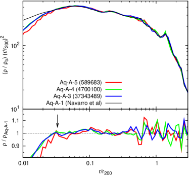
Figure 1: Spherically averaged density profiles of Aq-A-3,4 and 5 at $z=0$. The comoving softening length of all simulations is the same ($\epsilon=3.4~{}{\rm kpc}$; note that $r_{200}=246$ kpc for this halo) but the particle number increases from Aq-A-5 to Aq-A-3 as shown by the values of $N_{200}$ in the figure. The lower panel shows the difference between these profiles and that presented by Navarro et al. (2010) for Aq-A-1, for which $N_{200}\sim 10^{9}$. The convergence between the different resolutions is very good. All begin to fall below Aq-A-1 for $r<0.025r_{200}=6$ kpc because of the larger softening of our GDE resimulations. An arrow in the lower panel indicates 8 kpc, the radial position of the Sun within the Milky Way.

To integrate the comoving distortion tensor, we need to derive its equations of motion. We start with the physical GDE equation

$$\dot{\overline{\overline{D}}}=\overline{\overline{T}}~{}\overline{\overline{D}},$$ (7)

and introduce the peculiar potential field

$$\phi=a\Phi+\frac{a^{2}\ddot{a}}{2}\underline{x}^{\prime 2},$$ (8)

which is related to the density field via Poisson’s equation

$$\underline{\nabla}_{x^{\prime}}^{2}\phi=4\pi G\left(\rho^{\prime}(\underline{x}^{\prime})-\rho_{b}^{\prime}\right),$$ (9)

where $\rho_{b}^{\prime}$ denotes the comoving mean background density and the Laplacian is taken in comoving space. We note that the force field driving the motion of simulation particles is also derived from this peculiar potential. Since the GDE is directly related to the equations of motion of the particles themselves, it is natural to introduce a peculiar configuration-space tidal tensor $\underline{\underline{T}}^{\prime}$ with components $T_{ij}^{\prime}=-\partial^{2}\phi/\partial x_{i}^{\prime}\partial x_{j}^{\prime}$

$$\frac{1}{a^{3}}\underline{\underline{T}}^{\prime}=\underline{\underline{T}}-\frac{\ddot{a}}{a}\underline{\underline{1}}.$$ (10)

We can use this tidal tensor to write the equations of motion for the comoving distortion tensor in the following form

$$\dot{\underline{\underline{D}}}_{x^{\prime}q^{\prime}}^{\prime}=\frac{1}{a^{2}}\underline{\underline{D}}_{v^{\prime}q^{\prime}}^{\prime}, \quad\dot{\underline{\underline{D}}}_{x^{\prime}p^{\prime}}^{\prime}=\frac{1}{a^{2}}\underline{\underline{D}}_{v^{\prime}p^{\prime}}^{\prime},$$ (11)

$$\dot{\underline{\underline{D}}}_{v^{\prime}q^{\prime}}^{\prime}=\frac{1}{a}\underline{\underline{T}}^{\prime}\underline{\underline{D}}_{x^{\prime}q^{\prime}}^{\prime}, \quad\dot{\underline{\underline{D}}}_{v^{\prime}p^{\prime}}^{\prime}=\frac{1}{a}\underline{\underline{T}}^{\prime}\underline{\underline{D}}_{x^{\prime}p^{\prime}}^{\prime}.$$

Thus, the equations of motion for the comoving distortion tensor have exactly the same form as those for the physical one. The only difference is the appearance of the scale factor $a$ in the comoving equations. The initial conditions for these equations follow from those for the physical distortion tensor, taking into account $\overline{\overline{C}}_{\overline{x}^{\prime}\rightarrow\overline{x}}~{}\overline{\overline{C}}_{\overline{x}\rightarrow\overline{x}^{\prime}}=\overline{\overline{1}}$

$$\underline{\underline{D}}_{x^{\prime}q^{\prime}}^{\prime}(t_{\rm initial})=\underline{\underline{1}}, \quad\underline{\underline{D}}_{x^{\prime}p^{\prime}}^{\prime}(t_{\rm initial})=\underline{\underline{0}},$$ (12)

$$\dot{\underline{\underline{D}}}_{x^{\prime}q^{\prime}}^{\prime}(t_{\rm initial})=\underline{\underline{0}}, \quad\dot{\underline{\underline{D}}}_{x^{\prime}p^{\prime}}^{\prime}(t_{\rm initial})=\underline{\underline{1}}.$$

Based on these equations we can construct kick- and drift-operators for the leapfrog time integrator, similar to those for the position and velocity in the comoving frame.

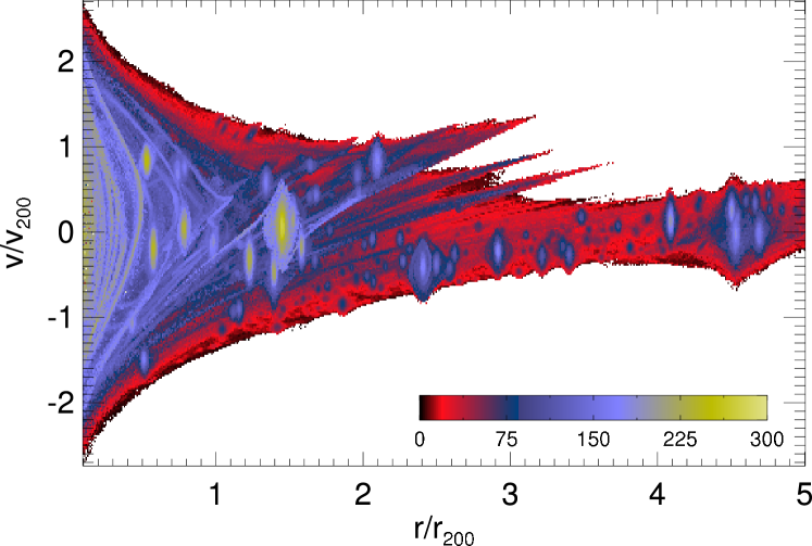
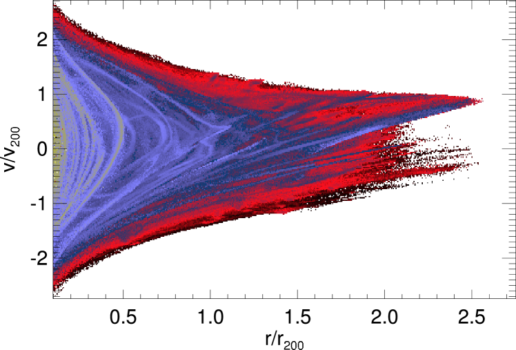
Figure 2: Top panel: Phase-space structure of the Aq-A-3 halo at $z=0$. Colour encodes the number of caustics passed by each individual simulation particle with the largest numbers plotted last. Subhaloes clearly stand out in this plot, because shorter orbital times lead to a higher number of caustic passages in their centres. We note that the streams visible in this plot are not fine-grained streams, but rather tidal streams resulting from disrupted subhaloes. Particles previously associated with subhaloes have higher caustic counts than other neighboring main halo particles, so they stand out in this phase-space portrait. Bottom panel: Same as the top panel, but with all bound subhaloes removed so that only the main halo component remains. Tidal streams from disrupted subhaloes are now more clearly visible. Note that this plot only shows particles bound to the main halo, while the top panel includes all particles within $5~{}r_{\rm 200}$. This is why the main halo contribution ends at about $2.5~{}r_{\rm 200}$. The colour scales for the two panels are the same, as indicated in the top panel.

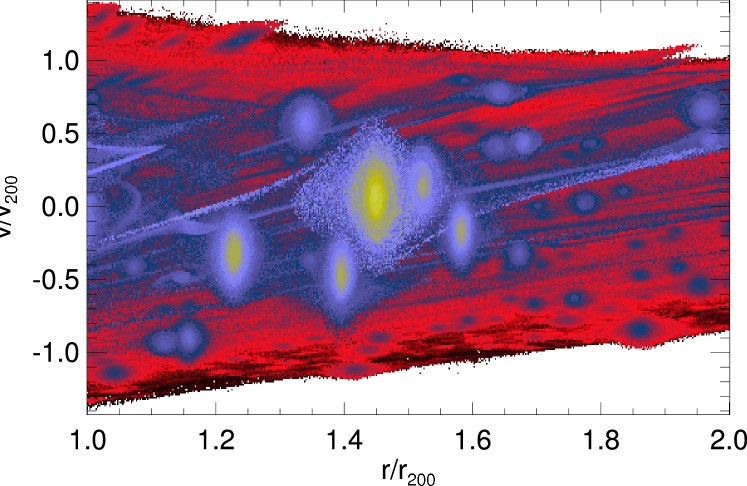
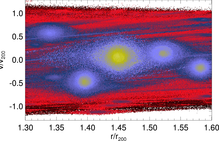
Figure 3: Two magnifications of the phase-space structure of Aq-A-3 focusing on one of the prominent subhaloes. The colour scale is the same as in Fig. 2. The tidal streams again stand out very clearly.

Let us now discuss how to derive stream densities from these comoving quantities. Each stream density is associated with a particular simulation particle, and describes the local density of the fine-grained stream it is embedded in. Our goal is to derive an equation that yields the physical stream density from the comoving distortion tensor discussed above. To begin, we note that the configuration-space distortion tensor can be derived from the phase-space distortion tensor by applying two projection operators as follows

$$\underline{\underline{D}}=\left(\underline{\underline{1}}\quad\underline{\underline{0}}\right)\overline{\overline{D}}\left(\begin{array}[]{c}\underline{\underline{1}}\\ \underline{\underline{V}}_{q}\end{array}\right),$$ (13)

where $\underline{\underline{V}}_{q}=\partial{\underline{V}}/\partial{\underline{q}}$ is the spatial gradient of ${\underline{V}}({\underline{q}})$, the mean initial sheet velocity as a function of initial position (see White & Vogelsberger, 2009, for a more formal definition). Caustic passages can be identified by sign changes in the determinant of this tensor. We note that this is true both in physical and in comoving space. The physical stream density can be calculated from the volume stretch factor implied by this linear transformation in physical configuration-space

$$\rho_{s}=\frac{\rho_{s,0}}{\left|\mathrm{det}\left(\underline{\underline{D}}\right)\right|},$$ (14)

as we described in Vogelsberger et al. (2008). Using $\rho_{s,0}=\rho_{s,0}^{\prime}/a(t_{\rm initial})^{3}$ and defining the peculiar velocity gradient $\underline{\underline{V}}_{q^{\prime}}^{\prime}=\underline{\underline{V}}_{q}-H(t_{\rm initial})\underline{\underline{1}}$ we can write the physical stream density as:

$$\rho_{s}=\frac{\rho_{s,0}^{\prime}}{a^{3}\left|\mathrm{det}\left[\underline{\underline{D}}_{x^{\prime}q^{\prime}}^{\prime}+a(t_{\rm initial})^{2}~{}\underline{\underline{V}}_{q^{\prime}}^{\prime}~{}\underline{\underline{D}}_{x^{\prime}p^{\prime}}^{\prime}\right]\right|}.$$ (15)

At early times when the dark matter is nearly uniform, all velocities and thus all velocity gradients are small and the second term in the determinant in this equation is small compared to the first. Thus we may approximate

$$\rho_{s}=\frac{\rho_{s,0}^{\prime}}{a^{3}\left|\mathrm{det}\left(\underline{\underline{D}}_{x^{\prime}q^{\prime}}^{\prime}\right)\right|}.$$ (16)

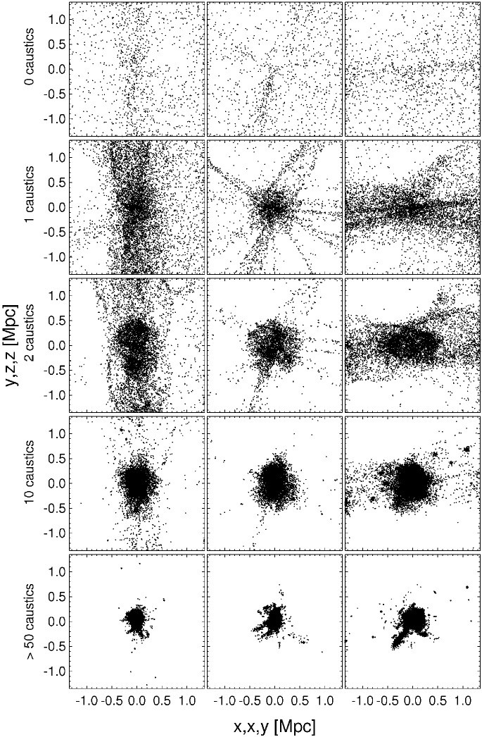
Figure 4: Slices of thickness $0.1~{}{\rm Mpc}$ through (xy, xz, yz) projections of the particle distribution in Aq-A-5, filtered by the number of caustics passed. The first four rows match the exact caustic passage number indicated, whereas the last row filters for particles that have passed more than $50$ caustics. The degree of structure in the different panels increases with the number of caustics passed. Particles that have not passed any caustic form a smooth distribution compared to the other panels of the figure.

This equation is sufficiently accurate for our purposes and we will use it below to calculate the stream densities associated with each particle in our simulations. For consistency we will also neglect the (small) initial variations in density and will assume the cosmological mean value everywhere, i.e.

$$\rho_{s,0}=\frac{3{H(t_{\rm initial})}^{2}}{8\pi G}.$$ (17)

3 Quantifying fine-grained halo structure

The results in the next few subsections are based on resimulations of the Aq-A halo at resolution levels 3, 4 and 5. We note again that our simulations use a significantly larger softening length than the original Aquarius simulations in order to mitigate the numerical noise sensitivity of the GDE. Unless otherwise stated, we use a Plummer-equivalent comoving softening length of $3.4~{}{\rm kpc}$. Note that we do not change softening between the different resolution levels that we are going to discuss. We will demonstrate that we reach convergence at level 4 with this set-up. Additional experiments show that this is the smallest softening length for which we could achieve convergence at this resolution level; smaller values require a larger particle number to converge. In the Appendix we show that our results for fine-grained stream densities (but not for caustic counts) are sensitive to the assumed softening because of its effect on the central structure of halo and subhalo potentials. Where needed, we also assume a dark matter particle with a velocity dispersion of $0.03~{}{\rm cm}/{\rm s}$ today. This corresponds to a neutralino of mass $100~{}{\rm GeV/c^{2}}$ that decoupled kinetically at a temperature around $10$ MeV.

To get started we show in Fig. 1 the spherically averaged density profile of the Aq-A halo at redshift $z=0$ for all three resolution levels. Note that $r_{200}=246$ kpc for this halo. Convergence is excellent over the full radial range plotted, as is more obvious in the lower panel where we plot the difference between our profiles and that given by Navarro et al. (2010) for the highest resolution simulation Aq-A-1. Softening clearly effects all three of our simulations similarly and only in the innermost regions; the deviation is at the percent level at the radius corresponding to the Sun’s position within the Milky Way, but reaches 10% by 4 kpc. Navarro et al. (2010) made similar convergence tests for the radial profiles of a variety of quantities in the original simulations.

3.1 Caustic counts

Our focus in this paper is not on the coarse-grained but on the fine-grained structure of our haloes. We begin by looking at the distribution of the number of caustics passed by particles in Aq-A. Caustics are identified through changes in the sign of the determinant of the comoving configuration-space distortion tensor and are counted along the trajectory of each particle. In Fig. 2 (top panel) we show the distribution of this caustic count in a phase-space diagram at $z=0$ for Aq-A-3. Colour encodes the number of caustics passed by each particle, as indicated by the colour bar. The particles were sorted by their caustic count before plotting, so that the particle with the highest caustic count is plotted in each occupied pixel. This phase-space diagram can be compared directly to the one in Vogelsberger et al. (2009b) which shows an isolated halo which grew from a spherically symmetric and radially self-similar perturbation of an Einstein-De Sitter universe. In both cases the number of caustic passages increases towards the centre of the halo, due to the shorter dynamical timescales in the inner regions: caustic count is roughly proportional to the number of orbits executed by each particle, because caustics occur near orbital turning points. The most important difference between the isolated and $\Lambda$CDM haloes is in the subhaloes and associated tidal streams seen in the $\Lambda$CDM case. Subhaloes stand out clearly in Fig. 2 since their particles have short orbital periods and undergo many caustic passages.

In the bottom panel of Fig. 2 we eliminate self-bound subhaloes to show only particles belonging to the main halo. Here tidal streams corresponding to disrupted subhaloes can be traced very well. Material from such disrupted subhaloes has a different caustic count distribution than other main halo material, and so stands out in these phase-space plots. In Fig. 3 we show two zooms into the phase-space structure around the most prominent subhalo of Fig. 2. These show the structure of the tidal streams in more detail. We note that these tidal streams are not equivalent to the fine-grained streams we will discuss below. As we will see, the latter are not visible in such phase-space plots because of their large number and their low densities.

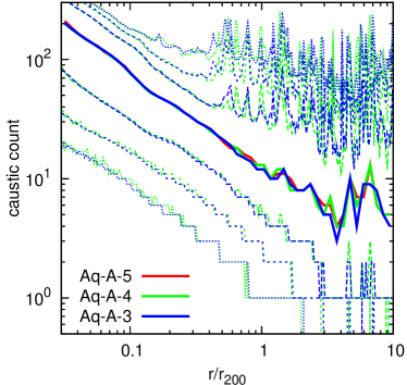
Figure 5: Median number of caustic passages (solid thick lines) in Aq-A as a function of radius. In the outer regions subhaloes show up as peaks. The convergence between the different resolutions is very good. Thin lines show the upper and lower $25\%$, $5\%$ and $1\%$ quantiles of the caustic count distribution in each radial bin for Aq-A-3 and Aq-A-4. The agreement between the distributions is excellent, at all radii except for some shifts at high counts in the outer regions which reflect small offsets in the positions of substructures. Clearly, caustic identification is stable against discreteness effects at these resolutions.

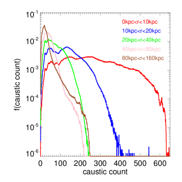
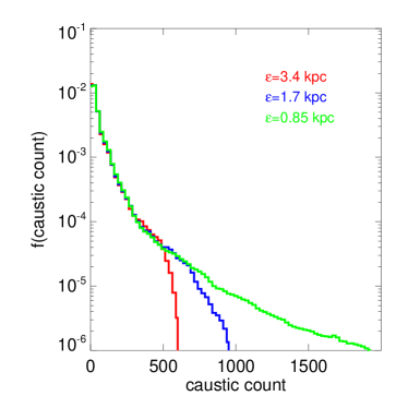
Figure 6: Top panel: Distribution of number of caustic passages at $z=0$ for particles in a set of nested spherical shells in Aq-A-3 for our standard softening of $3.4$ kpc. As expected, higher caustic counts are found in the inner regions. Bottom panel: Caustic count distributions within 160 kpc for Aq-A-3 resimulations with various softenings. The smaller the softening length, the longer the tail of high-count particles. The particles affected are almost all in the innermost region of the the main halo. Note that aside from this tail, the histograms are almost independent of softening.

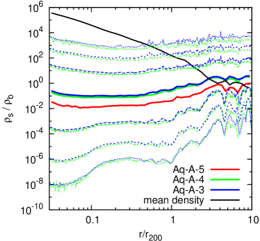
Figure 7: The distribution of stream density in units of the cosmic mean density ($\rho_{b}$) as a function of radius within halo Aq-A. Continuous coloured curves give the median stream density of particles as a function of their distance from halo centre for Aq-A-3 (blue), Aq-A-4 (green) and Aq-A-5 (red). Dashed and dotted curves give the 0.5, 2.5, 10, 90, 97.5 and 99.5% points of the distribution of stream density at each radius for Aq-A-3 (blue) and Aq-A-4 (green). The stream density distributions of the two higher resolution simulations agree well, but Aq-A-5 gives somewhat lower stream densities (for all percentiles, not just the median shown) as a result of its higher discreteness noise, We conclude that the resolution of Aq-A-4 is sufficient to suppress 2-body relaxation and other discreteness effects to an acceptably small level. Note that, remarkably, the median stream density is within an order of magnitude of the cosmic mean at all radii. For comparison, the black solid curve repeats the mean mass density profile of the halo from Fig. 1. Note that although the distribution of stream density spans twelve orders of magnitude in the inner halo, fewer than 1% of dark matter particles are in streams with densities exceeding 1% of the local mean.

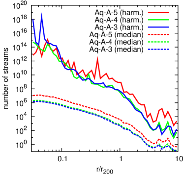
Figure 8: The number of streams in Aq-A as a function of radius, as estimated from the fine-grained stream densities of individual simulation particles. As in Fig. 7, the Aq-A-5 results disagree with those from the two higher resolution simulations, but Aq-A-3 and Aq-A-4 agree reasonably well. Stream numbers are estimated by dividing the mean density at each radius by an estimate of the characteristic local density of individual streams. For this estimate we use both the harmonic mean (solid lines) and the median (dashed lines) stream density for particles in each radial shell. The harmonic mean is very sensitive to the low density tail of the stream density distribution, but the agreement between Aq-A-3 and Aq-A-4 remains good except at the smallest radii.

Caustic counts can be used to study how dynamical mixing is related to particle location. To this end, we filter the particle distribution by number of caustic passages and plot the result in three orthogonal projections in Fig. 4. The top row of this figure shows that particles that have passed no caustic are almost homogeneously distributed, with no clear structure. Particles that have passed exactly one caustic already delineate the large-scale structure of the density field. The main filament passing through the primary halo is visible, as is the halo itself and additional smaller filaments pointing towards it. The halo is even more dominant in the distribution of particles that have passed two or ten caustics. The bottom row of Fig. 4 shows particles that have passed at least $50$ caustics. These are found only near the centres of the main halo and of the more massive subhaloes. These are the densest regions with the shortest orbital times. Typical values of the caustic count in various regions thus indicate their level of dynamically mixing. Large values correspond to well-mixed regions whereas small numbers correspond to dynamically “young” regions. Particles that have passed no caustic are still in the quasilinear phase of structure growth.

We can compress the caustic count information in a radial profile. This is shown in Fig. 5. Profiles of the median caustic count for Aq-A-3,4 and 5 are plotted as solid curves. As already demonstrated in Vogelsberger et al. (2008), the numerical identification of caustics is very robust, and as a result the number of caustic passages is little affected by numerical noise. This is why the median profile is almost independent of resolution in Fig. 5, with remarkably good agreement in the inner halo. In the outer regions subhaloes show up as peaks in the caustic count and small shifts in their position between the different simulations show up as apparent noise. For the highest resolution simulation, Aq-A-3, we also plot the upper and lower 1, 5 and 25% points of the count distribution at each radius. These parallel the distribution of the median count and span an order of magnitude at each radius. The median profile can be compared to that given by Vogelsberger et al. (2009b) for an isolated halo growing from self-similar initial conditions. At a given fraction of the virial radius, the typical number of caustic passages is only a few times larger in the more complex $\Lambda$CDM case.

The increase in caustic count towards halo centre can also be seen in Fig. 6 (top panel), where we present count histograms for particles in a set of nested spherical shells. The shift of the distributions towards lower counts with increasing radius is very obvious, and within about 30 kpc this is accompanied by a suppression of the high-count tail. At larger radii, however, the distributions always extends out to about 200 counts. This tail is contributed by particles from present or recently disrupted subhaloes (see below). In the outer halo, the majority of particles have nevertheless passed relatively few caustics. As noted above, simulations using the GDE technique require significantly more gravitational softening than standard N-body simulations in order to limit discreteness noise in the tidal field which otherwise leads to an unphysical, nearly exponential decay in stream density. Caustic identification is, however, relatively stable against such effects, so when studying caustic counts it is possible to reduce the softening. We show the effects of this in the bottom panel of Fig. 6 which compares the caustic count distribution within 0.16 Mpc in our standard resimulation with that in two additional resimulations with two and four times smaller softening. Smaller softening results in better resolution of the innermost regions both of the main halo and of subhaloes, and thus to shorter dynamical times and larger caustic counts for particles orbiting in these regions. This is evident as an extension of the high-count tail with decreasing softening. Notice, however that the region affected is more than two orders of magnitude below the peak of the distribution. The shift towards higher counts only affects a few percent of particles that pass close to halo centre, and the distribution is essentially unaffected below a count of about 400.

3.2 The distribution of fine-grained stream density

In the standard CDM paradigm, nonlinear evolution in the dark matter distribution can be viewed as the continual stretching, folding and wrapping of an almost 3-dimensional “phase-sheet” which initially fills configuration space almost uniformly and is confined near the origin in velocity space (see, for example White & Vogelsberger, 2009). Caustics are one generic prediction of such evolution. Another is that the phase-space structure near a typical point within a dark matter halo should consist of a superposition of streams, each of which has extremely small velocity dispersion and a spatial density and mean velocity which vary smoothly with position. If the number of streams at some point, for example at the position of the Sun, is relatively low, the resulting discreteness in the velocity distribution could give rise to measurable effects in an energy-sensitive detector of the kind used in many dark matter experiments. To assess this possibility, we need to estimate the number and density distributions of streams at each radius. Our GDE formalism makes this possible by providing a value for the density of the fine-grained stream associated with each simulation particle. The set of stream densities corresponding to particles within some spherical shell is thus a (mass-weighted) Monte Carlo sampling of the stream densities at that radius.

In Fig. 7 we show the distribution of fine-grained stream density as a function of radius in halo Aq-A. Continuous curves give radial profiles at $z=0$ for the median stream density of particles at three numerical resolutions, while broken curves compare the tails of the distributions for the two highest resolutions. Agreement is excellent at all radii and throughout the distribution for Aq-A-3 and Aq-A-4, but the lower resolution simulation Aq-A-5 gives lower stream densities at all radii (and at all points in the distribution, although we do not show this in order to avoid confusing the plot). This is a consequence of discreteness noise in the tidal tensor which affects integration of the GDE. We note that Fig. 5 and Fig. 7 demonstrate that the caustic count and stream density distributions are independent of particle number at our two highest resolutions. Thus, discreteness effects, in particular 2-body relaxation, have no significant influence on the evolution. In the Appendix we show that while the caustic count distribution is, in addition, independent of the assumed gravitational softening, the same is not true for the stream density distribution. This is because softening influences the tidal forces on particles which pass within one or two softening lengths of the centre of a halo or subhalo, and so influences the evolution of their stream density. As we discuss in the Appendix, this affects a surprisingly large fraction of halo particles at some point during their evolution, skewing the stream density distribution out to quite large radii. For our standard softening length of 3.4 kpc, the effects are similar in amplitude to those expected from our neglect of the baryonic component, so we do not attempt to correct for them.

A remarkable result from Fig. 7 is that the median stream density depends very little on radius, and is within an order of magnitude of the cosmic mean density at all radii. We found a very similar result in Vogelsberger et al. (2009b) for collapse from self-similar and spherically symmetric initial conditions, so it is likely to apply quite generally to collisionless, nonlinear collapse from a smooth and near-uniform early state. It implies that the dark matter distribution from the immediate neighborhood of a randomly chosen point in the early universe is almost equally likely to be compressed or diluted relative to the cosmic mean by subsequent nonlinear evolution, and furthermore that whether it is compressed or diluted is almost independent of its final distance from halo centre.

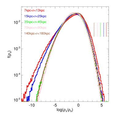
Figure 9: Histograms of fine-grained stream density at $z=0$ for Aq-A-3 particles in set of spherical shells. Labels with the colour of each histogram give the radial range of the corresponding shell, while vertical dotted lines correspond to the mean halo density within that shell. All histograms are normalised to integrate to unity.

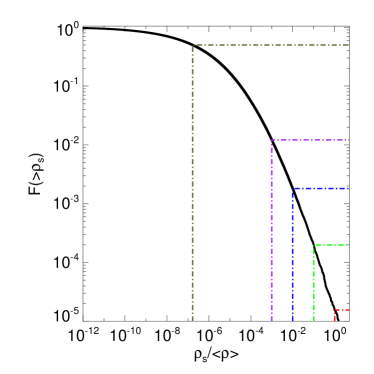
Figure 10: The fraction of particles in Aq-A-3 at $z=0$ with halocentric radii in the range $7$ to $13$ kpc which have fine-grained stream density exceeding $\rho_{s}$ is plotted as a function of $\rho_{s}/\langle\rho\rangle$, where $\langle\rho\rangle$ is the mean halo density at $10$ kpc. Half of all particles are in streams with $\rho_{s}>10^{-7}\langle\rho\rangle$. See the text for a discussion of the other characteristic points marked.

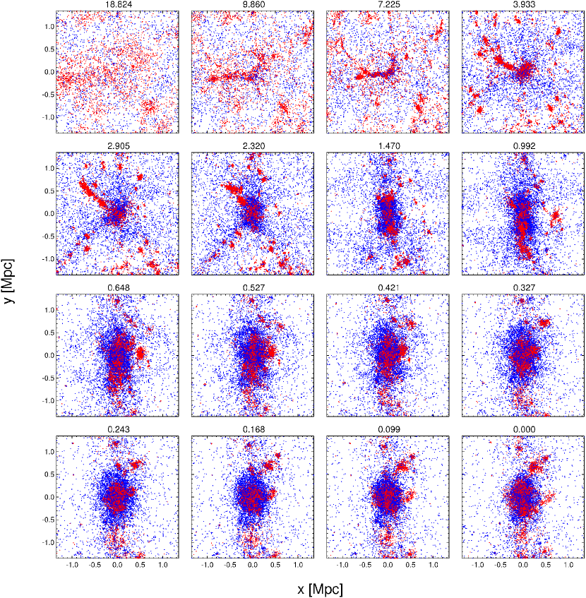
Figure 11: The panels show a series of snapshots from the evolution of Aq-A-5. The redshift is indicated above each panel. Red and blue points refer to the same particles in each panel and are plotted in random order so that the probability of a random pixel being red or blue in a saturated region is proportional to the number of particles of each colour in that pixel. The particles were selected by separating the full $z=0$ particle distribution into a series of thin spherical shells centred on the main halo potential centre, and then choosing in each shell the 1% tails with the highest (blue) and lowest (red) stream density. Blue and red particles are thus equal in number and at $z=0$ each population is distributed in distance from halo centre in the same way as the particle distribution as a whole. Only particles within $10~{}r_{\rm 200}$ at $z=0$ were considered. The comoving cubic region plotted lies fully within this particle set at all times and is centred on the centre of mass of the 200 particles which were most bound at $z=0$. Clearly, low $z=0$ stream density particles typically belong to collapsed structures at early times, whereas high stream density particles were generally part of no structure before they were accreted smoothly onto the main halo at relatively late times.

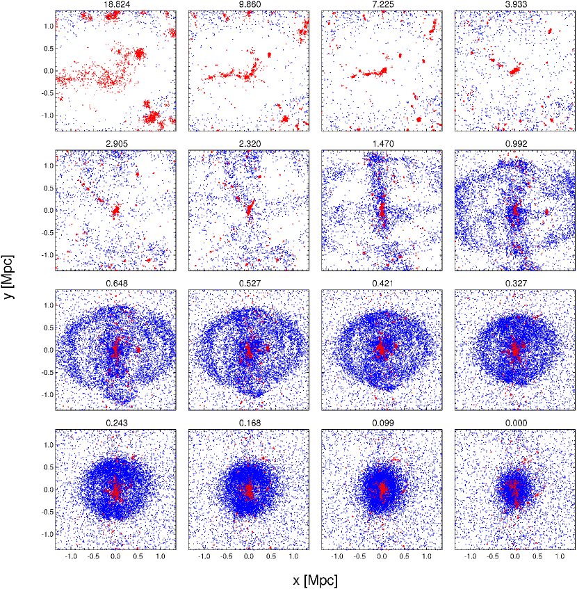
Figure 12: This figure was constructed in exactly the same way as Fig. 11 and shows the same number of red and blue particles at the same redshifts and within the same spatial regions. The difference is that particles were here selected on the basis of the number of caustics they have passed by $z=0$, rather than by their present-day stream density. Thus, for the same set of thin spherical shells as before, red particles are the 1% within each $z=0$ shell with the highest caustic count, and the blue particles are the 1% with the lowest caustic count (random sampled if necessary among particles with equal count to obtain exactly the correct number). Thus the number of red and blue points in the lower right panel of this figure and of Fig. 11 is the same, and they have exactly the same distribution in halocentric radius. The small apparent number of red points in most panels of this figure is due to the fact that high $z=0$ caustic count particles are strongly concentrated to the centres of collapsed structures at all times. The relatively small number of blue points at the earliest redshifts in this figure reflects the fact that many blue particles are outside the region plotted at early times. The qualitative behaviour of the distributions in this figure and in Fig. 11 is similar, but the separation into high spatial density and near-uniform distributions is much more marked when particles are selected by caustic count rather than by stream density. In addition, low caustic count particles are accreted onto the final halo in a shell-like pattern which is a clear reflection of the structure seen in spherical infall models of halo formation.

The thin dashed and dotted lines in Fig. 7 show the 0.5, 2.5, 10, 90, 97.5 and 99.5% points of the stream-density distribution as a function of distance from the centre of our Aq-A-3 and Aq-A-4 simulations. This distribution is very broad, spanning almost 12 orders of magnitude near halo centre. Despite this, within $0.5r_{200}$ even the upper 0.5% tail of stream densities lies below the mean density of the halo which is shown as a solid black curve for comparison. At 8 kpc, the equivalent of the Solar radius, fewer than 1% of all dark matter particles are part of a fine-grained stream with density exceeding 1% of the local mean halo density. This is a first indication that fine-grained streams are unlikely to influence direct detection experiments strongly.

The total number of streams at a typical point in a radial shell can be estimated from the stream density distribution as the ratio of the mean halo density in the shell to the harmonic mean of the stream densities of the particles it contains. This number is dominated by the extended low-density tail of the stream-density distribution; a very large number of very low-density streams is predicted in the inner regions. A more relevant measure for dark matter detection can be obtained from the median stream density of the particles. Half of all events in a dark matter detector will come from streams with densities exceeding this value, and so will come from a number of streams somewhat less than half the ratio of the mean halo density to this median value.

In Fig. 8 we show the results of such calculations for our resimulations of Aq-A at various resolutions. Solid lines show the total number of streams at each radius estimated from the harmonic mean stream density, whereas dashed lines show the number of “massive” streams estimated from the median individual stream density. The two estimates differ dramatically, particularly in the inner halo, reflecting the very broad distribution of stream densities at each radius, and in particular the presence of simulation particles with very low stream densities. As in Fig.7, convergence is somewhat poorer than for the caustic count statistics we looked at above, but the results for Aq-A-3 and Aq-A-4 nevertheless agree remarkably well. This is particularly notable for the solid lines, given the sensitivity of the harmonic mean to the low-density tail of the distribution. From Fig. 8 we estimate the total number of streams at halocentric radii near that of the Sun to be around $10^{14}$ and the number of “massive” streams to be about $10^{6}$. Clearly CDM haloes are predicted to be very well mixed in their inner regions, and the velocity distribution near the Sun should appear very smooth. The very large number of streams predicted near the Sun’s position can be understood from the analysis in Vogelsberger et al. (2008), which shows that stream density should fall inversely as the number of caustic passages in a one-dimensional system, but as the cube of this number for regular orbits in a three-dimensional system, and even faster for chaotic orbits. Given that typical particles near the Sun have passed a few hundred caustics, typical stream densities are predicted to be $\sim 10^{-7}\rho_{b}$. The local mass overdensity at the solar position is $\sim 10^{5}$, so one predicts $\sim 10^{12}$ fine-grained streams passing through our vicinity. Additional scatter is introduced by the fact that a significant fraction of the particles are “pre-processed” in smaller mass systems before they fall into the main halo.

We show the distribution of stream densities in a different form in Fig. 9. For a series of spherical shells with mean radii increasing by factors of two, we have made histograms of the fine-grained stream densities of Aq-A-3 particles, normalising them to unity so that their shapes can be compared. Beyond 30 kpc these histograms are all quite similar, and resemble slightly skewed log-normal distributions. At the bottom of our plot, three orders of magnitude below peak, they span 14 orders of magnitude in stream density. At smaller radii, the low-stream-density tail becomes more extended, the peak of the distribution shifts very little, and the shape of the high-stream-density tail is unchanged. The latter is determined by the behaviour near caustics. As we will see below the maximum densities at caustics are predicted to be in the range explored by this high-mass tail. It is notable that within 20 kpc these tails do not extend up to the local mean density of the halo.

The implications of these distributions for direct detection experiments on Earth are most easily drawn from Fig. 10, which shows the cumulative distribution of fine-grained stream density for Aq-A-3 particles with $7~{}{\rm kpc}<r<13~{}{\rm kpc}$ at $z=0$. Specifically, we plot the fraction of particles with stream density exceeding $\rho_{s}$ against $\rho_{s}/\langle\rho\rangle$, where $\langle\rho\rangle$ is the mean halo density at 10 kpc. The fraction of particles with $\rho_{s}>\langle\rho\rangle$ is about $2\times 10^{-5}$, so the probability that a single stream dominates the signal in a direct detection experiment (i.e. that the Earth lies sufficiently close to a sufficiently strong caustic) is about $2\times 10^{-5}$. The fraction of particles with $\rho_{s}>0.1\langle\rho\rangle$ is about $2\times 10^{-4}$, hence the probability to see a single stream containing 10% of the signal is about 0.002. Similarly, the fraction of particles with $\rho_{s}>0.01\langle\rho\rangle$ is about $2\times 10^{-3}$, so a single stream containing 1% of the signal will be seen with probability 20%. Finally, the fraction of particles with $\rho_{s}>0.001\langle\rho\rangle$ is about $10^{-2}$; this means that at a typical “Earth” location there will be a few streams which individually contribute more than 0.1% of the local dark matter density. Thus an experiment which registers 1000 true dark matter “events” should get a few duplicates, i.e. events coming from the same fine-grained stream and so having (very nearly) the same velocity. If the dark matter is made of axions then a resonant detector should find an energy spectrum where a few tenths of a percent of the total energy density is concentrated in a few very narrow “spectral lines”.

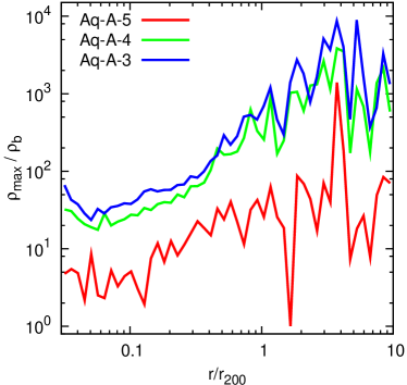
Figure 13: Top panel: Radial profile of the median value of peak caustic density for simulations at three different resolutions. The resolution of Aq-A-5 is too low to get converged results, but the results from Aq-A-4 and Aq-A-3 agree quite well. Bottom panel: The mean halo density profile of Aq-A-3 is compared to the median and the quartiles of the peak density of caustics as a function of radius. Beyond the virial radius, typical caustics have peak densities which exceed the local mean density. Caustics in the inner halo have very low contrast, however.

3.3 Origin of the tails of the stream density and caustic count distributions

Given the very broad range of stream densities and caustic counts present at each point within our haloes, it is interesting to investigate how these properties are related to the dynamical history of individual particles. We begin by studying stream density.

As we saw above, the “typical” stream density of particles (specifically, the local median value) is almost independent of local mean halo density, thus of local dynamical time. Lower stream density corresponds to greater stretching of the initial phase-sheet and so, one might think, to more effective dynamical mixing. An anticorrelation of fine-grained phase density with local orbital time (i.e. with radius) is, however, at most marginally evident in the stream density distributions of Fig. 7 and then only in their low-stream-density tails. To a first approximation there is no correlation between stream density distribution and radius. The overall mean density profile of the halo is built up by having more streams of every density at smaller radii. Thus the relation of stream density to dynamical mixing is far from evident.

Figure 14: Local ratio of the spherically averaged intra-stream annihilation rate to the spherically averaged smoothed annihilation rate as a function of radius. The smoothed annihilation rate is calculated from a SPH-based density estimate using 64 neighbours. The intra-stream annihilation rate is dominated by contributions around caustics. The standard “boost factor” due to unbound small-scale structure is one plus the quantity plotted on the vertical axis. Clearly, caustics play essentially no role in enhancing the dark matter annihilation luminosity of the inner halo. Around the virial radius they contribute about $10\%$ to the annihilation signal.

We explore this issue in Fig. 11. Red and blue points here highlight the positions at a series of redshifts of particles which at $z=0$ lie within $10~{}r_{\rm 200}$ of halo centre. We divided this region into a set of thin nested spherical shells and then for each shell we identified particles in the upper and lower 1% tails of the stream density distribution. The particles with the highest $z=0$ stream densities (which are typically close to caustics) are plotted blue in each panel while those with the lowest stream densities (which are typically in collapsed regions and far from caustics) are plotted red. Thus at $z=0$ there are the same number of red and blue points in the plot, and both populations are distributed in halocentric radius exactly as the mass distribution as a whole. The spatial distributions of the two populations differ markedly, however, both at $z=0$ and at all earlier times. Most of the red particles are part of clumps already at early times, while most of the blue particles either appear diffuse or are distributed relatively smoothly through the main halo at all times. There is thus indeed a correlation between stream density and dynamical history, despite the lack of correlation between stream density and halocentric distance in Fig. 7.

The number of caustic passages is a clearer measure of dynamical mixing, because it is closely related to the number of orbits a particle has executed over its entire dynamical history. We examine this using Fig. 12 which is constructed in exactly the same way as Fig. 11 except that the particles in each $z=0$ spherical shell were ranked by caustic count rather than by stream density. Qualitatively the two series of plots show some similarities, but the differences between the red and blue populations are substantially more marked in the caustic count case. The red points are almost all very close to the centres of collapsed clumps at all times, whereas the blue population is always diffuse except at low redshift when some of it is accreted onto the main halo. The evolution of the blue particles in Fig. 12 shows an interesting shell-like structure which can be understood with reference to a spherical infall model. Many of the blue particles have yet to pass a caustic at $z=0$, and so are on their first passage through the halo. Such particles come from a narrow range of Lagrangian radii in the initial conditions, hence the apparent shell. The fact that the caustic count is a much better indicator of the overall level of dynamical mixing than the stream density is easily understood; the stream density varies strongly along the trajectory of each individual particle reaching high values each time it passes a caustic, whereas the caustic count increases monotonically with the number of orbits completed.

3.4 Caustics and dark matter annihilation

The number of fine-grained streams passing through the Solar System is of interest for the search for dark matter using laboratory devices. Caustics, on the other hand, could be of interest for indirect dark matter searches that focus on the annihilation products of dark matter particles. Annihilation explanations for many of the apparent “anomalies” in indirect detection signals, for example the rise in the positron fraction detected by PAMELA above the expectation from secondary production, require annihilation rates to be substantially “boosted” above predictions based on “standard” particle physics assumptions and haloes with a locally smooth dark matter density field. The annihilation rate per unit volume is proportional to the square of the local dark matter density and so can reach very high values in caustics. Caustics could thus, at least in principle, provide the necessary boost. To quantify this with our simulations, it is important not only to identify caustics, but also to estimate their peak densities, since emission around the peak dominates caustic luminosity (see White & Vogelsberger, 2009).

In Fig. 13 we plot median peak caustic density as a function of radius for Aq-A. To make this plot we recorded the peak caustic density and the radial position at which it was achieved for all particles that pass through a caustic in a short time interval around $z=0$. We bin these caustic passages into a set of radial shells, and then find the median value of peak caustic density for each shell. The top panel shows results at three different resolutions, Aq-3, Aq-A-4 and Aq-A-5. Again, it is clear that the lower resolution of Aq-A-5 has significantly affected the results, while Aq-A-3 and Aq-A-4 agree reasonably well. The peak caustic density calculation, like that of the stream density, depends on the full phase-space distortion tensor, so it is not surprising that the convergence properties of the two measures are similar. In the bottom panel we compare the spherically averaged mass density profile of Aq-A-3 with the radial distribution of peak caustic density. The thick red line repeats the median profile from the top panel, while thin blue lines show the upper and lower quartiles of peak caustic density as a function of radius. Notice that at each radius the distribution of peak caustic densities is very broad, mirroring the range of fine-grained stream densities seen in Fig. 7. The peak densities of almost all caustics in the inner part of the halo are substantially below the local mean halo density. A quarter of all caustics have peak densities exceeding the local mean at about $0.4r_{200}$, but only outside $0.8r_{200}$ do more than half of the caustics have peak densities higher than the local mean density.

The low peak densities predicted for caustics in the inner halo, suggest that any annihilation boost will be small. This was already the case for the isolated, smoothly growing halo studied in Vogelsberger et al. (2009b). In a $\Lambda$CDM halo, additional small-scale structure should decrease stream densities, and thus peak caustic densities, even further. To investigate this, we calculate the ratio of intra-stream annihilation (both particles belonging to the same fine-grained stream) to inter-stream annihilation (the two particles belonging to different fine-grained streams). The former can be calculated for each simulation particle from its GDE-estimated stream density and can be integrated correctly through caustics using the formalism of White & Vogelsberger (2009). The latter can be calculated from a SPH kernel estimate of the local smooth dark matter density. For the boost to be substantial the ratio of these two annihilation rates should be large. In Fig. 14 we plot this ratio for Aq-A as a function of radius, after averaging the rates over thin spherical shells. Again, results for Aq-A-3 and Aq-A-4 agree well, while those for Aq-A-5 are clearly affected by its low resolution. This reflects the similar effects seen in earlier plots of stream and caustic densities. Fig. 14 shows that the contribution of caustics to the overall annihilation luminosity is very small – boosting is completely negligible in the inner halo, and is still small (about a factor of 1.1) near the virial radius. This is even lower than the already small effects seen in the smooth halo collapse simulation presented by Vogelsberger et al. (2009b). Since an annihilation interpretation of the PAMELA results requires a boost factor of 100 to 1000, caustics are clearly far too weak to provide an explanation. Since bound subhaloes are also unable to produce local boosts much above unity near the Sun (Springel et al., 2008b), non-standard particle physics such as Sommerfeld enhancement (e.g. Sommerfeld, 1931; Hisano et al., 2004; Hisano et al., 2005; Cirelli et al., 2007; Arkani-Hamed et al., 2009; Lattanzi & Silk, 2009) must be invoked to explain the PAMELA data through annihilation.

3.5 Object-to-object scatter

In the last few subsections we discussed the fine-grained structure of Aq-A in considerable detail and studied how it is affected by numerical resolution. It is not, of course, clear how representative these results are, since they are based on a single Milky Way-like halo. To quantify the scatter expected as a result of variations in formation history, environment, etc., it is important to check some of these properties for other haloes. The Aquarius Project simulated six Milky Way-mass haloes at very high resolution, and so provides an opportunity to address this issue. The question of how representative these particular haloes are of the full population of similar mass objects is discussed by Boylan-Kolchin et al. (2009). Here, we concentrate on the caustic count profile which we showed in Fig.5 to be very well converged in Aq-A-3, Aq-A-4 and Aq-A-5, at least within $r_{200}$ where the “noise” due to substructure is small. Given this robust result, we decided for the following comparison to rerun the other five Aquarius haloes at resolution level 4 in order to save computation time. All resimulations were carried out with our standard softening length of $3.4$ kpc.

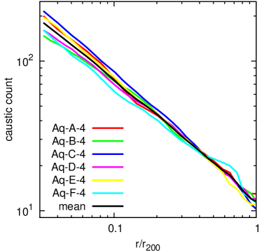
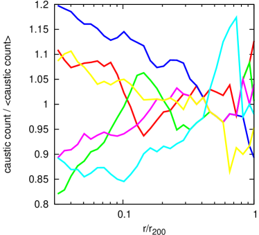
Figure 15: Top panel: Radial profiles of median caustic count similar to that in Fig.5 but for all six Aquarius haloes resimulated at resolution level 4 with a softening of 3.4 kpc. We plot only the region interior to $r_{200}$ in order to exclude the substantial “noise” at larger radii due to individual massive subhaloes. Bottom panel: Ratio of the individual halo caustic count profiles to their mean.

In the top panel of Fig. 15 we show profiles of median caustic count as a function of radius for all six Aquarius haloes. We plot results within $r_{200}$ only, since at larger radii the profiles are subject to large stochastic fluctuations at the positions of massive subhaloes (see Fig.5). The variations between the six haloes are relatively small and are systematic with radius as can be seen in the lower panel of Fig. 15 where we plot the ratio of each of the individual profiles to their mean. Differences are largest in the central regions but still scatter by less than 20% around the mean. There is some correlation of the caustic count profile with the radial mass density profile. Haloes A and C have the most concentrated mass density profiles (see Boylan-Kolchin et al. (2009)) and also have the highest caustic counts in the inner regions, as might naively be expected. Halo E, on the other hand, is the least concentrated of all the haloes and yet also has a relatively high caustic count near the centre. Clearly, the details of halo assembly history do affect the median number of caustic passages significantly. This is not determined purely by the local dynamical time of the final halo.

In Fig. 16 we do the same exercise for the number of streams. For each of our resimulated Aquarius haloes we use the median stream density of the particles at each radius to estimate a characteristic stream number, as in the dashed curves of Fig. 8 which demonstrate that good convergence is achieved at resolution level 4. We plot the profiles out to $2r_{200}$ in this case; at larger radii stochastic effects due to massive subhaloes again dominate the variations. The top panel shows the profiles themselves, while the lower panel plots the ratio of each individual profile to their (geometric) mean. Halo-to-halo differences here are larger than for the caustic counts, but still relatively modest given the large dynamic range of the radial variation. It is interesting that the ranking of haloes here is similar but not identical to that in the caustic count profiles of Fig. 15; the most concentrated haloes A and C not only have the largest caustic counts in their inner regions, but also the smallest numbers of streams. This is unexpected since a naive argument might have led one to expect that a larger number of caustics would correspond to a larger number of streams.

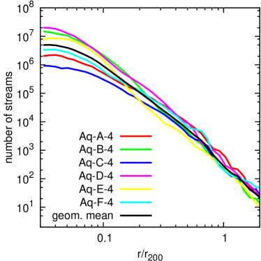
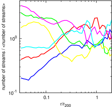
Figure 16: Top panel: Stream number, defined as for the dashed curves of Fig. 8, for the six Aquarius haloes at level 4 resolution and with our fiducial softening length of $3.4$ kpc. We plot out to $2r_{200}$ since at larger radii these profiles are affected by individual massive subhaloes. Bottom panel: Ratio of the individual halo stream number profiles to their (geometric) mean.

4 Concluding remarks

We have demonstrated how N-body simulation techniques can be extended to follow fine-grained structure and the associated caustics during the formation of dark matter haloes from fully general $\Lambda$CDM initial conditions. We have shown that, for the large particle numbers of our standard experiments, our integrations of the geodesic deviation equation (GDE) produce distributions of fine-grained stream density and caustic structure which are independent of particle number, hence insensitive to discreteness effects such as two-body relaxation. This requires somewhat larger gravitational softenings than are used in traditional N-body simulations, and we show in the Appendix that while caustic count distributions are insensitive to the assumed softening, the same is not true for the stream density distributions. We have resimulated the six Milky Way-mass haloes of the Aquarius Project, allowing us to analyse the scatter in fine-grained properties among haloes of similar mass.

By identifying caustic passages along its trajectory, we are able to assign a cumulative caustic count to each simulation particle which is robust against numerical noise and serves to indicate the extent of dynamical mixing in its phase-space neighborhood. This caustic count provides an excellent means to highlight subhaloes and tidal streams in $r$–$v_{r}$ phase-space plots, because particles which became part of condensed structures at early times complete more orbits, and so pass more caustics than particles which remain diffuse until accreted onto the main halo. Filtering the particle distribution by caustic count decomposes it into interpenetrating components which have experienced different levels of dynamical mixing. Particles that have passed no caustic form an almost uniform subcomponent, while particles with large caustic count (e.g. $>50$) are found only in the dense inner regions of haloes. Particles with intermediate count outline the skeleton of the cosmic web.

Direct dark matter detection experiments are, in principle, sensitive to the fine-grained structure of the Milky Way’s halo at the position of the Sun. It is especially important to know if a significant fraction of the local dark matter density could be contributed a one or a few fine-grained streams, since each of these would be made of particles of a single velocity with negligible dispersion. If many streams contribute to the local density and none is dominant, then a smooth velocity distribution can be assumed. Our simulations show the unexpected result that the distribution of fine-grained stream density is almost independent of radius within the virialised region of dark matter haloes. Only the low-density tail of the distribution appears to extend downwards at small radii. Because of the extreme breadth of the distribution, a very large number of streams ($\sim 10^{14}$) is predicted at the Solar position, but about half of the total local dark matter density is contributed by the $10^{6}$ most massive streams. The most massive individual stream is expected to contribute about 0.1% of the local dark matter density. This is potentially important for axion detection experiments which have extremely high energy resolution and may be able to detect 0.1% of the total axion energy in a single “spectral line”. Apart, from this possibility, dark matter detection experiments may safely assume the velocity distribution of the dark matter particles to be smooth.

It has been suggested that the very high local densities associated with caustics might significantly enhance dark matter annihilation rates in dark matter haloes, and thus be of considerable significance for indirect detection experiments. Indeed, for completely cold dark matter it can be shown that the contribution from caustics is logarithmically divergent and hence dominant (Hogan, 2001). This divergence is tamed by the small but finite initial velocity dispersions expected for realistic CDM candidates, and calculations for idealised, spherical self-similar models indicate quite modest enhancements for standard WIMPs (Mohayaee & Shandarin, 2006). Our methods allow us to identify all caustics during halo formation from fully general $\Lambda$CDM initial conditions. We find that they are predicted to make a substantially smaller contribution to the local annihilation rate than in the spherical model. This is because the more complex orbital structure of realistic haloes results in lower densities for typical fine-grained streams and thus to lower caustic densities when these streams are folded. The enhancement due to caustics near the Sun is predicted to be well below $0.1\%$ and so to be completely negligible. Only in the outermost halo does the enhancement reach 10%. The standard N-body technique of estimating annihilation rates from SPH estimates of local DM densities (see, for example, Springel et al., 2008b) should therefore be realistic, and such estimates will not be significantly enhanced by caustics. Similarly, caustics cannot be invoked to provide the large boost factors required by annihilation interpretations of ‘anomalies’ in recently measured cosmic ray spectra from the PAMELA or ATIC experiments. Given that unresolved small subhaloes also appear insufficient to provide a substantial boost (Springel et al., 2008b), an annihilation interpretation of these signals is only tenable with nonstandard annihilation cross-sections.

Our comparison of results for the six different haloes of the Aquarius Project showed that the halo-to-halo variation in the fine-grained properties we have studied is relatively small, and thus does not have significant impact on the applicability of our principal conclusions to the particular case of our own Milky Way. Thus our final conclusion must be that the fine-grained structure of $\Lambda$CDM haloes has almost no influence on the likelihood of success of direct or indirect dark matter detection experiments.

Although we demonstrated that two-body relaxation and other discreteness effects have no significant influence on our conclusions, we found that our predicted stream density distributions are strongly affected by gravitational softening, which modifies the tidal forces on particles passing within a softening length or two of halo centre. This numerical effect remains a significant uncertainty in our results. The analysis in the Appendix shows that reducing the softening below our standard value tends to reduce the density of streams, thus to suppress further the importance of fine-grained structure for detection experiments. However, the change in orbit structure induced by our standard softening is similar in scale and amplitude to that caused by the neglected baryonic components of the galaxies, and even the sign of the effect of the latter is uncertain. This is clearly an area where further work is required to reduce the remaining uncertainty in our quantitative conclusions.

Appendix A Effects of gravitational softening

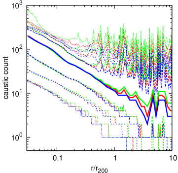
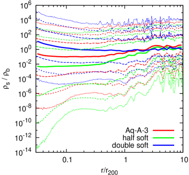
Figure 17: Top panel: Distribution of caustic passages in Aq-A-3 as a function of radius and of gravitational softening. Thick lines show the median and thin lines the upper and lower $25\%$, $5\%$ and $1\%$ quantiles of the caustic count distribution at each radius. Red lines refer to our standard simulation with our fiducial softening length of $\epsilon=3.4~{}{\rm kpc}$. Green and blue lines show results for softening lengths half and twice this value, respectively. Clearly softening does not significantly affect these distributions. Bottom panel: The distribution of stream density in Aq-A-3 (in units of the cosmic mean) as a function of radius and of gravitational softening. Continuous curves give the median, and dashed and dotted lines the 0.5, 2.5, 10, 90, 97.5 and 99.5% points of the distribution at each radius. Red curves correspond to our fiducial softening length of $\epsilon=3.4~{}{\rm kpc}$, green and blue lines to softenings half and twice as big, respectively. The stream density distribution is significantly affected by gravitational softening at all radii, although the effect gets weaker in the outer halo.

According to Figs. 5 and 7 the caustic count and stream density distributions are independent of particle number at our two highest resolutions. This demonstrates that discreteness effects, in particular two-body relaxation, are not significantly affecting the phase-space quantities we derive from our GDE integrations. In this Appendix we investigate whether these distributions are sensitive to our assumed gravitational force softening. To facilitate this, we keep the particle number fixed and change the softening length. Specifically, we resimulated Aq-A-3 using softening lengths half and and twice our fiducial value, $\epsilon=3.4~{}{\rm kpc}$, but with all other parameters held to their original values.

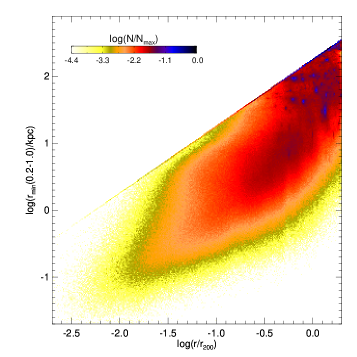
Figure 18: Distribution of halo particles at $z=0$ in the $r/r_{200}$ versus $r_{\rm min}(0.2-1)$ plane for the Aq-A-4 simulation with half our fiducial softening, i.e. $\epsilon=1.7~{}{\rm kpc}$. Even at large radius, a surprisingly large fraction of particles have minimal pericentric distance within one or two softening lengths.

The top panel of Fig. 17 shows that the caustic count distribution is independent of softening in the main halo, but that its high count tail is affected by softening in subhaloes. Subhaloes are effectively small $N$ systems, and their centres are significantly better resolved with a smaller softening length. This results in larger caustic counts at the centre of subhaloes, which are evident as enhanced “noise” in the high-count tail at larger radii for the simulation with the smallest softening. This effect is almost absent in the main halo. We conclude that our main results for caustic counts are robust to changes in softening length, a conclusion supported by the results of Vogelsberger et al. (2008).

The bottom panel of Fig. 17 shows a similar plot but now for the stream density distribution. Here we see a very different result. The stream density distribution depends quite strongly on softening, with smaller softenings resulting in a shift of the entire stream density distribution towards lower values. The effect is largest at small radii but is evident throughout the main halo. In the inner halo the median stream density drops by more than three orders of magnitude when the softening length is reduced by a factor of 4. The difference is even larger if we focus on the low-density tail of the distribution and is still quite substantial in the high-density tail.

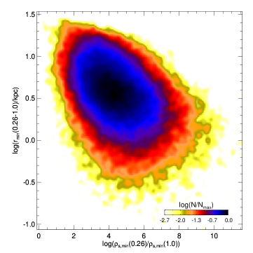
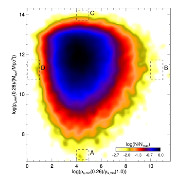
Figure 19: Two-dimensional histograms of properties of a particle subset defined by the following criteria: halocentric distance at $z=0$ between $0.01~{}r_{200}$ and $r_{200}$; number of caustic passages from $a=0.26$ to $a=1$ between $38$ and $42$; already part of the main subhalo (i.e. not part of any identified subhalo) at $z=2.9$. Top panel: Distribution in the $\rho_{\rm s,min}(0.26)/\rho_{\rm s,min}(1)$ versus $r_{\rm min}(0.26-1)$ plane. Particles with smaller minimum radius over the $z=2.9$ to $z=0$ period typically decrease their stream density by a larger factor, i.e. $\rho_{\rm s,min}(0.26)/\rho_{\rm s,min}(1)$ tends to be larger for smaller $r_{\rm min}(0.26-1)$. Bottom panel: Distribution in the $\rho_{\rm s,min}(0.26)/\rho_{\rm s,min}(1)$ versus $\rho_{\rm s,min}(0.26)$ plane. There is no correlation between the two quantities. Within this particle set, the change in stream density after $z=2.9$ is independent of a particle’s prior history. Notice also that the distribution of the change in stream density is broader than the initial distribution, showing that the final stream density distribution is determined primarily by effects during the redshift interval considered. The small boxes labelled A to D select particles at the edges of the distribution. In Fig. 20 we plot the evolution of stream density and halocentric distance for six particles chosen at random from each box.

To understand the origin of this effect, we repeated the Aq-A-4 simulation with half the fiducial softening and stored the particle data at all $\sim 7000$ time-steps between $z=4$ and $z=0$. This allows us to follow the orbit and the phase-space density evolution of each particle in detail. We find the $200$ most bound particles at $z=0$ and use their centre-of mass position to define the halo centre at all earlier times. (We checked that they are all indeed still very close to halo centre at $z=4$.) For every halo particle we then construct trajectories of halocentric distance and fine-grained stream density, and define a minimum physical halocentric distance over any chosen scale factor interval ($r_{\rm min}(a_{1}-a_{2})$), and a minimum physical stream density achieved between $z=4$ and any later epoch ($\rho_{\rm s,min}(a)$). Fig. 18 shows the $z=0$ distribution of all particles in the $r/r_{200}$ versus $r_{\rm min}(0.2-1)$ plane. This histogram shows the expected trend that particles at small $z=0$ radii tend to have passed closer to halo centre in their past than particles at large $z=0$ radii. Interestingly, the typical minimum radius is more than an order of magnitude smaller than the final radius, and the scatter in the distribution is quite large. Thus at a third the virial radius (around 80 kpc) the distribution peaks at a closest approach distance of about 3 kpc, thus within our fiducial softening length. At a tenth the virial radius, most particles have passed within 1.0 kpc of halo centre. Thus, everywhere within the halo a significant fraction of particles have passed through a region where tidal forces are substantially affected by the softenings we are using. The tidal field sources evolution in the GDE, so this affects our stream density estimates. Specifically, particles feel stronger shearing at pericentre if the softening length is smaller, so we expect larger stream density decrements for smaller softenings.

To investigate this further, we select a subset of particles according to the following criteria: halocentric distance at $z=0$ between $0.01~{}r_{200}$ and $r_{200}$; caustic count increment from $a=0.26$ to $a=1$ between $38$ and $42$; part of the main halo (i.e. not part of any resolved subhalo) at $a=0.26$. This selects a set of particles with similar orbital periods which have all been part of the main body of the system since $z=2.9$. The top panel of Fig. 19 shows the distribution of these particles in the $\rho_{\rm s,min}(0.26)/\rho_{\rm s,min}(1)$ versus $r_{\rm min}(0.26-1)$ plane. The ratio $\rho_{\rm s,min}(0.26)/\rho_{\rm s,min}(1)$ indicates the decrease in minimal physical stream density between $z=2.9$ and $z=0$, which, as expected, is strongly correlated with minimum halocentric distance. Particles with stream density changes substantially smaller than the median have typically never been closer to the centre than 2 or 3 kpc, while particles with substantially larger than average changes in stream density have almost all been within 3 kpc of halo centre, many within 1 kpc. The bottom panel of Fig. 19 shows the same particle set in the $\rho_{\rm s,min}(0.26)/\rho_{\rm s,min}(1)$ versus $\rho_{\rm s,min}(0.26)$ plane, i.e. the drop in physical stream density from $z=2.9$ to $z=0$ versus the initial stream density at $z=2.9$. There is no correlation between these quantities, showing that the change in stream density after $z=2.9$ is independent of what happened to the particle at earlier times. In addition, the distribution of stream density changes is broader than the initial distribution, showing that the main features of the final distribution were established over the time interval considered.

Together these plots show that, for this particle subset, low stream densities at $z=0$ are associated almost exclusively with particles that pass within our fiducial softening length of the centre some time after $z=2.9$. Even in the main part of the stream density distribution about half of the particles pass within 3 kpc of halo centre. As we will see below, the time-average halocentric distance of these particles is about 40 kpc. This explains why changing our softening between 1.7 and 6.8 kpc has effects out to large radii, as seen in the stream density distributions of Fig. 17, and why the effects are stronger near halo centre and in the low-density tail of the distribution.

The stored data for our test simulation allow us to trace the detailed evolution of stream density for individual particles. We illustrate this for a few particles in the extreme regions of the distribution labelled A to D in the bottom panel of Fig. 19. We pick $6$ particles at random from each region and plot in Fig. 20 their physical stream density and physical halocentric distance as a function of scale factor. These plots demonstrate that particles in fully general CDM halos show quite similar stream density behaviour to those in simpler halo models: caustic “spikes” occur several times per orbit at turning points of the fundamental oscillations, and secular evolution is evident in the steady decrease in the minimum stream densities achieved between caustic passages. This resembles the isolated halo results in Vogelsberger et al. (2008), showing that our GDE scheme works correctly in the cosmological setup of this paper. The selection criteria for our particle subset are evident in the similar apocentric distances and similar caustic and pericentric passage numbers of all orbits, despite their very different initial and final stream densities.

The stream density decrease is different in the four regions, reflecting their location in the $\rho_{\rm s,min}(0.26)/\rho_{\rm s,min}(1)$ versus $\rho_{\rm s,min}(0.26)$ plane. Our GDE approach finds stream densities spanning almost $18$ orders of magnitude for orbits of very similar size and period. The orbits in regions A and C look similar both in their stream density and in their radial orbit behaviour. The only difference is an offset of about 6 orders of magnitude in stream density which is preserved throughout the evolution. This emphasises that evolution from $z=2.9$ to $z=0$ is independent of what happened before $z=2.9$ if one restricts oneself to main halo particles with similar orbital periods. The particles in boxes B and D also have similar orbital periods, but they now have similar initial stream densities and very different stream density evolution. Those in box D barely change their stream density over the period shown, while the stream densities of those in box B drop by about 11 orders of magnitude. Here there are clear qualitative differences in orbital structure. The particles in box D avoid the halo centre and in some cases are almost circular, and their caustics are relatively uniformly spaced in time and show rather little variation. In contrast, the particles in box B make much larger radial excursions, often passing close to the centre, and their caustic structure is more variable with caustic passages often occurring in groups. This suggest that further work on the structure of the stream density evolution curves might allow classification of the orbits into tubes, boxes and other families.

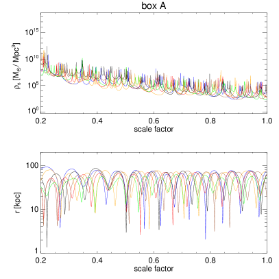
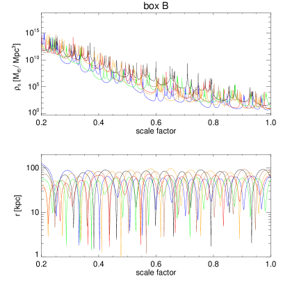
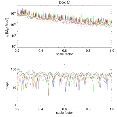
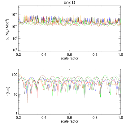
Figure 20: Stream density and halocentric distance (both physical) as a function of scale factor for six particles randomly selected from each of the regions labelled A to D in the bottom panel of Fig. 19. Each particle has its own colour which corresponds in each pair of plots.

References

- Abdo et al. (2009) Abdo A. A., et al. M., 2009, Physical Review Letters, 102, 181101
- Adriani et al. (2009) Adriani O., Barbarino G. C., Bazilevskaya e. a., 2009, Nature, 458, 607
- Arkani-Hamed et al. (2009) Arkani-Hamed N., Finkbeiner D. P., Slatyer T. R., Weiner N., 2009, Phys. Rev. D, 79, 015014
- Bergström (2009) Bergström L., 2009, New Journal of Physics, 11, 105006
- Bergström et al. (2008) Bergström L., Bringmann T., Edsjö J., 2008, Phys. Rev. D, 78, 103520
- Bernabei et al. (2008) Bernabei R., et al., 2008, European Physical Journal C, pp 167–+
- Bernabei et al. (2010) Bernabei R., et al., 2010, European Physical Journal C, pp 39–+
- Bertone et al. (2005) Bertone G., Hooper D., Silk J., 2005, Phys. Rep., 405, 279
- Boylan-Kolchin et al. (2009) Boylan-Kolchin M., Springel V., White S. D. M., Jenkins A., 2010, MNRAS, 406, 896
- Cirelli et al. (2007) Cirelli M., Strumia A., Tamburini M., 2007, Nuclear Physics B, 787, 152
- Diemand et al. (2008) Diemand J., Kuhlen M., Madau P., Zemp M., Moore B., Potter D., Stadel J., 2008, Nature, 454, 735
- Diemand et al. (2005) Diemand J., Moore B., Stadel J., 2005, Nature, 433, 389
- Finkbeiner et al. (2009) Finkbeiner D. P., Lin T., Weiner N., 2009, Phys. Rev. D, 80, 115008
- Gelmini (2006) Gelmini G. B., 2006, Journal of Physics Conference Series, 39, 166
- Gondolo & Gelmini (2005) Gondolo P., Gelmini G., 2005, Phys. Rev. D, 71, 123520
- Green et al. (2005) Green A. M., Hofmann S., Schwarz D. J., 2005, Journal of Cosmology and Astro-Particle Physics, 8, 3
- Hisano et al. (2004) Hisano J., Matsumoto S., Nojiri M. M., 2004, Physical Review Letters, 92, 031303
- Hisano et al. (2005) Hisano J., Matsumoto S., Nojiri M. M., Saito O., 2005, Phys. Rev. D, 71, 063528
- Hogan (2001) Hogan C. J., 2001, Phys. Rev. D, 64, 063515
- Hooper et al. (2007) Hooper D., Finkbeiner D. P., Dobler G., 2007, Phys. Rev. D, 76, 083012
- Jungman et al. (1996) Jungman G., Kamionkowski M., Griest K., 1996, Phys. Rep., 267, 195
- Lattanzi & Silk (2009) Lattanzi M., Silk J., 2009, Phys. Rev. D, 79, 083523
- Malyshev et al. (2009) Malyshev D., Cholis I., Gelfand J., 2009, Phys. Rev. D, 80, 063005
- Mohayaee et al. (2007) Mohayaee R., Shandarin S., Silk J., 2007, Journal of Cosmology and Astro-Particle Physics, 5, 15
- Mohayaee & Shandarin (2006) Mohayaee R., Shandarin S. F., 2006, MNRAS, 366, 1217
- Moore et al. (1999) Moore B., Ghigna S., Governato F., Lake G., Quinn T., Stadel J., Tozzi P., 1999, ApJ, 524, L19
- Natarajan & Sikivie (2006) Natarajan A., Sikivie P., 2006, Phys. Rev. D, 73, 023510
- Natarajan & Sikivie (2008) Natarajan A., Sikivie P., 2008, Phys. Rev. D, 77, 043531
- Navarro et al. (2010) Navarro J. F., et al. A., 2010, MNRAS, 402, 21
- Savage et al. (2004) Savage C., Gondolo P., Freese K., 2004, Phys. Rev. D, 70, 123513
- Sommerfeld (1931) Sommerfeld A., 1931, Annalen der Physik, 403, 257
- Springel (2005) Springel V., 2005, MNRAS, 364, 1105
- Springel et al. (2008a) Springel V., et al. J., 2008a, MNRAS, 391, 1685
- Springel et al. (2008b) Springel V., White S. D. M., Frenk C. S., Navarro J. F., Jenkins A., Vogelsberger M., Wang J., Ludlow A., Helmi A., 2008b, Nature, 456, 73
- Stadel et al. (2009) Stadel J., Potter D., Moore B., Diemand J., Madau P., Zemp M., Kuhlen M., Quilis V., 2009, MNRAS, 398, L21
- Vogelsberger et al. (2008) Vogelsberger M., White S. D. M., Helmi A., Springel V., 2008, MNRAS, 385, 236
- Vogelsberger et al. (2009a) Vogelsberger M., et al., 2009a, MNRAS, 395, 797
- Vogelsberger et al. (2009b) Vogelsberger M., White S. D. M., Mohayaee R., Springel V., 2009b, MNRAS, 400, 2174
- White & Vogelsberger (2009) White S. D. M., Vogelsberger M., 2009, MNRAS, 392, 281