The Effect of a Time-Varying Accretion Disk Size on Quasar Microlensing
Light Curves

Abstract

Microlensing perturbations to the magnification of gravitationally lensed quasar images are dependent on the angular size of the quasar. If quasar variability at visible wavelengths is caused by a change in the area of the accretion disk, it will affect the microlensing magnification. We derive the expected signal, assuming that the luminosity scales with some power of the disk area, and estimate its amplitude using simulations. We discuss the prospects for detecting the effect in real-world data and for using it to estimate the logarithmic slope of the luminosity’s dependence on disk area. Such an estimate would provide a direct test of the standard thin accretion disk model. We tried fitting six seasons of the light curves of the lensed quasar HE 0435$-$1223 including this effect as a modification to the Kochanek et al. (2006) approach to estimating time delays. We find a dramatic improvement in the goodness of fit and relatively plausible parameters, but a robust estimate will require a full numerical calculation in order to correctly model the strong correlations between the structure of the microlensing magnification patterns and the magnitude of the effect. We also comment briefly on the effect of this phenomenon for the stability of time delay estimates.

1. Introduction

Recent observational studies of the microlensing of gravitationally lensed quasars (see review by Wambsganss, 2006) have led to new constraints on the structure of the innermost regions of quasars and on the properties of foreground galaxies. Because quasar accretion disks subtend angles comparable to the Einstein radii of stars in foreground galaxies, studies taking advantage of the dependence of microlensing magnifications on the source size have been able to estimate the sizes of accretion disks (Pooley et al., 2007; Anguita et al., 2008; Dai et al., 2010; Morgan et al., 2010), and multi-wavelength observations have enabled estimates of the wavelength dependence of the disk size (Poindexter et al., 2008; Eigenbrod et al., 2008; Bate et al., 2008; Floyd et al., 2009; Mosquera et al., 2009). Other studies have estimated the ratio of clumpy stellar mass to more smoothly distributed dark matter in lensing galaxies, providing the only constraints on stellar mass fractions not dependent on the initial mass function (e.g. Pooley et al., 2009). Time domain observations of microlensing variability are a particularly powerful tool for this type of investigation. For example, they have been used recently to estimate the inclination of a quasar accretion disk (Poindexter & Kochanek, 2010a) as well as its transverse velocity relative to the lens and the mean mass of the stars in the lensing galaxy (Poindexter & Kochanek, 2010b).

To date, quasar microlensing has nearly always been modeled using accretion disks with time-independent sizes; this ought to be a good first-order approximation. But the fact that quasar luminosities are time-variable indicates that this model cannot hold in detail. Observationally, short-term variations in individual image fluxes have been observed for a few lensed quasars (Schild, 1996; Kundic et al., 1997; Schechter et al., 2003), leading to hypotheses involving microlensing of disks with fast-moving hot spots (Gould & Miralda-Escude, 1997; Schechter et al., 2003) or obscured by fast-moving optically thick broad-line clouds (Wyithe & Loeb, 2002).

In the spirit of these studies, we investigate a model of a time-varying accretion disk with a size proportional to some power of the quasar luminosity. This model introduces one new parameter, which is the exponent $\epsilon$ between the disk effective area and luminosity (i.e. $A\propto L^{\epsilon}$); for simple blackbody disks they are directly proportional ($\epsilon=1$). We show that observations of the light curves of multiply imaged quasars have the potential to detect this disk size variability, and discuss how such detections may be used to constrain the value of $\epsilon$. In Section 2 we outline the mathematical model for the observed light curve of a quasar image in terms of the intrinsic quasar light curve. In Section 3 we study the amplitude of the effect for a time-variable disk by simulating realistic microlensing scenarios. We describe in Section 4 an algorithm for measuring the effect in real-world light curves of lensed quasars, and report in Section 5 the results of applying it to the light curves of the quasar HE 0435$-$1223. In Section 6 we give a brief overview of our conclusions.

2. Mathematical model

The optical and near-infrared continuum luminosity of bright quasars is thought to arise in a thin accretion disk radiating as a multi-temperature blackbody (see review by Blaes, 2007). If the blackbody effective temperature varies as a power law with radius, $T_{\mathrm{eff}}=T_{0}(R/R_{0})^{-\beta}$, then by integrating the Planck function over all radii, the total luminosity of the disk can be shown to be proportional to $R_{0}^{2}K(\beta)$, where $K(\beta)$ is a dimensionless function of the power law slope. This calculation has been used as a means of estimating the disk size from the optical luminosity (e.g. Morgan et al., 2010), but our main concern is the scaling. The luminosity of a blackbody disk with a power-law temperature profile will scale linearly with its effective area $R_{0}^{2}$.

This scaling implies that quasar variability at ultraviolet and optical rest wavelengths is matched by a proportional variability in the size of the accretion disk. This is the simplest model for a time-variable disk size, because it does not require the introduction of substructure in the disk or any new time scale. In the case of quasars that are experiencing microlensing, the source size dependence of the microlensing magnification will affect an image’s light curve in phase with the quasar variability, boosting or suppressing it depending on the details of the microlens configuration.

To quantify the effect, we start with the observed flux of a lensed quasar image as a function of time,

$$f(t)=L(t)M+f_{C}~{},$$ (1)

where $L(t)$ is the time-dependent quasar luminosity and $M$ is the effective magnification — specifically, the product of the macro-magnification and the microlensing magnification. The latter can change with time, but for this first discussion we will assume that it is constant on the time scales of quasar variability. $M$ does, however, change with the area of the disk, because the microlensing magnification pattern is the convolution of the true caustic pattern with the (changing) source profile. The $f_{C}$ term denotes contaminating flux from non-disk sources, such as broad emission lines, the quasar host galaxy or the lens galaxy. The flux (and likewise the quasar luminosity $L$ and disk area $A$) may be decomposed into a DC component and a small time-variable component:

$$f(t)=\langle f\rangle+\delta f(t)~{},$$ (2)

where

$$\langle f\rangle =\langle ML\rangle(1+C)~{},~{}\mathrm{and}$$

$$\delta f(t) =\langle M\rangle\delta L(t)+\langle L\rangle\frac{dM}{dA}\delta A(t)~{}.$$ (3)

Here $C\equiv f_{C}/\langle ML\rangle$ is the fractional flux contamination. Thus,

$$\frac{\delta f}{\langle f\rangle}= \left(\frac{\delta L}{\langle L\rangle}+\frac{d\ln{M}}{d\ln{A}}\frac{\delta A}{\langle A\rangle}\right)\left(1+C\right)^{-1}$$

$$\approx \frac{\delta L}{\langle L\rangle}\left(1+\epsilon\frac{d\ln{M}}{d\ln{A}}-C\right)~{},$$ (4)

where $\epsilon\equiv(d\ln{L}/d\ln{A})^{-1}$ is the logarithmic change in disk luminosity with disk area. If the luminosity of the disk is simply proportional to its area, then $\epsilon=1$. We have assumed in the second line that $C\ll 1$, and that $d\ln{M}/d\ln{A}$ is also small (we verify this assumption in Section 3). To convert this expression to magnitudes, we first separate the light curve into a time-averaged component $\langle m\rangle=-2.5\log\langle f\rangle$ and a small variable component $\delta m(t)\propto\delta f/\langle f\rangle$. Thus

$$\delta m(t)\approx\delta m_{\mathrm{int}}(t)\left(1+\epsilon\frac{d\ln{M}}{d\ln{A}}-C\right)~{},$$ (5)

where $\delta m_{\mathrm{int}}(t)\propto\delta L/\langle L\rangle$ is the intrinsic time-variable light curve of the quasar. This intrinsic variability is identical for all the images of a lensed quasar (once lensing time delays have been accounted for). Thus, for a pair of images with low amounts of contaminating flux, a difference in $d\ln{M}/d\ln{A}$ will cause a difference in the amplitude of quasar variability seen in the two images. If the former is larger than a few percent, the latter ought to be detectable when comparing measured light curves. Observationally, for quasar images labeled A and B, the intrinsic light curve measured in image B, relative to that measured in A, would seem to be multiplied by the function

$$\zeta(t)=1+\epsilon\left[\left(\frac{d\ln{M}}{d\ln{A}}\right)_{B}-\left(\frac{d\ln{M}}{d\ln{A}}\right)_{A}\right]-C_{B}+C_{A}~{}.$$ (6)

3. Simulations

We calculated the probability distribution functions of the value of $d\ln{M}/d\ln{A}$ for several realistic microlensing parameter values. We also created an example of a simulated light curve that includes the effect of a time-varying disk, in order to test the validity of the assumptions we made in Section 2.

Figure 1.— Examples of the distributions of $d\ln{M}/d\ln{A}$ for a selection of macro-magnifications (shown at the upper right of each plot). The source half-light radius is fixed at $10^{-0.5}=32$% of a solar mass Einstein radius, and the stellar mass fraction is fixed at 10%.

For these simulations, we used magnification maps created using the inverse ray-shooting software of Wambsganss et al. (1990). The maps had a total surface mass density (or convergence) $\kappa_{\mathrm{tot}}$ roughly equal to their shear $\gamma$, divided into contributions from smooth matter and point masses. We specify a broken power-law mass function for the microlens stars. Between $0.08\,M_{\odot}$ and $0.5\,M_{\odot}$, its logarithmic slope is $-1.8$, and above $0.5\,M_{\odot}$ it steepens to $-2.7$. This mass function is very similar to that of Kroupa (2001). We cut off the mass function at $1.5\,M_{\odot}$, because lens galaxies are typically early-type galaxies with old stellar populations. With this mass function, the average microlens mass is $\langle m\rangle=0.247\,M_{\odot}$, in reasonable agreement with the recent measurement by Poindexter & Kochanek (2010b).

Each map encodes the deviation in the magnification of its quasar image from that produced by a smooth mass distribution as a function of the position of the source. They are $2000$ pixels on a side; this is $20$ times the Einstein radius of a solar-mass microlens star. When projected back to the quasar, the side length is $\sim 5\times 10^{17}$ cm (the exact number depends on the redshifts of the lens and the quasar), and the pixel size is thus $\sim 2.5\times 10^{14}$ cm, or a few gravitational radii for a $10^{9}\,M_{\odot}$ black hole. This is much smaller than the size of the optical accretion disk.

3.1. Histograms

For any particular quasar image, $d\ln{M}/d\ln{A}$ depends on the microlensing caustic pattern associated with that image and the size of the accretion disk. One can calculate a probability distribution for its value by first taking the difference of two copies of an appropriate pattern which have been convolved with source profiles of slightly different areas, dividing the result by the difference in the logarithm of those areas, and finally creating a histogram of the resulting pattern.

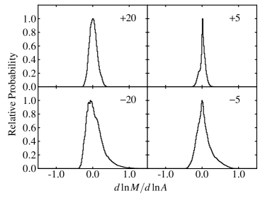
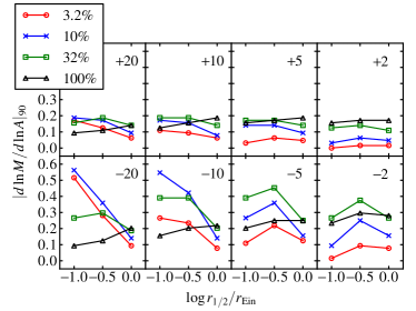
We created histograms for 8 macro-magnifications, 4 stellar fractions, and 3 source sizes that are typical of quasars lensed by foreground galaxies. We simulated finite-sized accretion disks by convolving the magnification maps with circular Gaussian profiles characterized by a half-light radius, a parameter which has been shown (Mortonson et al., 2005; Congdon et al., 2007) to be more important that the exact radial profile of the source. Each difference map was created by subtracting a map which had been convolved with a source 0.1 dex smaller (in each dimension) than the chosen size from a map convolved with a source 0.1 dex larger. Figure 1 shows four such histograms, although this is only a fraction of the 96 cases we considered. Figures 2 and 3 show the absolute value of $d\ln{M}/d\ln{A}$ bounding 50% and 90% of the probability in each histogram, respectively.

Figure 2.— 50% probability bounds on $|d\ln{M}/d\ln{A}|$ as a function of the ratio of the source half-light radius to a solar-mass Einstein radius. Macro-magnifications are shown in the upper right of each plot. The surface mass fraction in stars $\kappa_{*}/\kappa_{\mathrm{tot}}$ is indicated by the symbol shape, with a legend in the upper left.

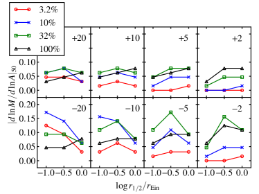
Clearly $d\ln{M}/d\ln{A}$ is a small fraction of unity for most magnifications, stellar fractions, and source sizes. However, there is significant probability that it will be large enough to have an observable effect, particularly for small sources in highly-magnified saddle-point images. We stress, however, that even for large sources, where the first-order effects of microlensing become very weak, there remains substantial probability for $d\ln{M}/d\ln{A}$ to have significantly nonzero value.

Figure 3.— 90% probability bounds on $|d\ln{M}/d\ln{A}|$ as a function of the ratio of the source half-light radius to a solar-mass Einstein radius. Macro-magnifications are shown in the upper right of each plot. The surface mass fraction in stars $\kappa_{*}/\kappa_{\mathrm{tot}}$ is indicated by the symbol shape, with a legend in the upper left. Note the change in vertical scale from Figure 2.

3.2. Light curve simulation

Our derivation in Section 2 assumed that the time scale for microlensing was long compared to the time scale for quasar variability. However, this is not always the case, as quasars can vary on a range of time scales (e.g. Kelly et al., 2009; Kozłowski et al., 2010) and microlens caustic crossings can happen quickly for smaller source sizes (e.g. Chartas et al., 2009). In order to test our mathematical description, we ran a more detailed simulation of the microlensing of a quasar whose area varied linearly with its flux.

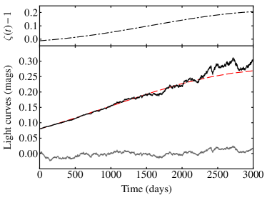
We generated an intrinsic light curve for the source using the damped random walk stochastic model introduced by Kelly et al. (2009) and extensively confirmed by Kozłowski et al. (2010) and MacLeod et al. (2010). An accretion disk with a Gaussian profile and a time-averaged half-light radius $10^{-0.2}=63$% the size of a solar-mass Einstein radius was run across two magnification maps, with a velocity of 1000 km s^-1 (projected on the source plane). The maps were chosen to simulate a high-magnification, merging pair of images with macro-magnifications of $\pm 20$ and stellar mass fractions $\kappa_{*}/\kappa_{\mathrm{tot}}=0.1$. We simulated 3000 epochs, each separated by a day. At each time step, the area of the source was adjusted proportionally to the intrinsic light curve, and the magnification maps were convolved with the resulting source to find the microlensing magnifications. The simulation produced observed light curves for the two quasar images which contained the imprint of the intrinsic quasar light curve as well as microlensing and the variation of the microlensing magnification with source area (i.e. $\zeta(t)$).

Figure 4 shows the difference between the resulting light curves, including the effect of a time-varying source size, and compares it to the same quantity with the source size held constant at the size associated with the mean flux. The first curve shows a clear echo of the intrinsic source light curve, modulated by $\zeta(t)$ in good agreement with Equation 6.

Figure 4.— Bottom panel: Simulated difference light curve for a pair of highly magnified quasar images. The dashed curve shows the difference that would be observed if the disk size was held fixed at its average value. The solid black curve includes the effects of an accretion disk with a time-varying area. For comparison, at the bottom, we show in gray the input quasar light curve scaled by a “typical” $d\ln{M}/d\ln{A}$ factor of $0.1$ (see Figures 2 and 3). Top panel: Difference in $d\ln{M}/d\ln{A}$ between the two images, as a function of time. This is the factor controlling the “echo” of the intrinsic light curve seen in the difference curve in the bottom panel. The source’s average half-light radius is 63% of a solar-mass Einstein radius, and the stellar mass fraction is fixed at 10%. This simulation assumes perfect correction for the time delays between the images.

4. Measuring the effect

We adapted the time-delay fitting algorithm described by Kochanek et al. (2006) to fit for the presence of $\zeta(t)$ in measured light curves. This algorithm defines a model light curve consisting of the sum of a high-order polynomial $s(t)$ (representing the intrinsic quasar variability) and lower-order polynomials $\Delta\mu_{i}(t)$ (representing microlensing fluctuations). The intrinsic light curve is constrained to be the same for all lensed images, whereas the microlensing terms are allowed to vary. We modified Equation 3 of Kochanek et al. (2006) as follows:

$$\chi^{2}=\sum_{i=1}^{N_{\mathrm{im}}}\sum_{j=1}^{N_{\mathrm{obs}}}\left[\frac{m_{ij}-\zeta_{i}(t_{j})s(t_{j}+\Delta t_{i})-\Delta\mu_{i}(t_{j})}{\sigma_{ij}}\right]^{2}~{}.$$ (7)

Here $m_{ij}$ and $\sigma_{ij}$ are the data and errors, respectively, and each $\zeta_{i}(t)$ is parameterized by a low-order polynomial. (In practice, $\zeta_{i}(t)$ is multiplied by only the terms in $s(t)$ that are higher-order than $N_{\mu}$, the order of $\Delta\mu_{i}(t)$, to avoid degeneracy.) We used a Markov Chain Monte Carlo (MCMC) technique to minimize $\chi^{2}$ with respect to the time delays $\Delta t_{i}$ and the coefficients parameterizing $\zeta_{i}(t)$. At each step in the chain, the linear parameters of $s(t)$ and $\Delta\mu_{i}(t)$ were determined by minimizing the $\chi^{2}$ as in Kochanek et al. (2006). We fit the entire time series simultaneously, as opposed to breaking it into seasons, because we found that in practice this gave us better control over “cross-talk” between the microlensing terms and $\zeta(t)$.

We tested the efficacy of this technique by applying it to simulated light curves for 30 pairs of images. Like the simulations in Section 3.2, these curves started with a stochastic intrinsic light curve, but these did not contain microlensing variability; we simply multiplied one of each pair of intrinsic light curves by a slowly-varying curve representing $\zeta(t)$. We deleted from each light curve 140 out of every 365 points to simulate six observing seasons, and fit a model to the remaining data to determine the time delay and $\zeta(t)$. The latter was modeled using Legendre polynomials to quadratic order: $\zeta(t)=\sum_{i=0}^{2}b_{i}P_{i}(\hat{t})$, where $\hat{t}$ is a scaled time variable running from $-1$ at the beginning of the light curve to $1$ at its end. We used a quartic ($N_{\mu}=4$) to fit the microlensing component, and set the parameter $\lambda$ to 1.0. We varied the order of the source polynomial $N_{\mathrm{src}}$ between 120 and 190, and found a small decreasing trend in the average $\chi^{2}$ per degree of freedom for higher orders. However, the decrease was less than the scatter in the values, so we concluded that $N_{\mathrm{src}}=120$ was sufficient. On average, the algorithm successfully recovered the $b_{i}$ and time delay parameters. Table 1 compares the mean of the 30 best-fit values to the true parameter values, and gives the scatter in the best-fit values and their typical formal uncertainty.

Table 1Best-fit simulated $\zeta(t)$ parameters

	$b_{0}$	$b_{1}$	$b_{2}$	$\Delta t$ (days)
True value	$1.10$	$0.11$	$-0.05$	$\mbox{$\phantom{-}$}0.00$
Mean	$1.11$	$0.11$	$-0.05$	$-0.07$
Standard deviation	$0.02$	$0.05$	$\mbox{$\phantom{-}$}0.08$	$\mbox{$\phantom{-}$}0.66$
Typical uncertainty	$0.02$	$0.05$	$\mbox{$\phantom{-}$}0.06$	$\mbox{$\phantom{-}$}0.42$

Note. — Errors represent formal 68% ($\Delta\chi^{2}=1$) confidence intervals.

These tests demonstrate that measurements of $d\ln{M}/d\ln{A}$ in real-world lensed quasars have the potential to constrain the value of $\epsilon$, that is, the relationship between accretion disk size and luminosity. If the values that are measured (e.g. using the above method) fall in significantly unlikely regions of the theoretical histograms (see Section 3.1), the $\epsilon=1$ hypothesis, that is, a blackbody with power-law temperature profile, will be called into question.

The presence of contaminating light from non-disk sources in our quasar image light curves acts as a spurious offset in the measured $\zeta(t)$ curves (see Equation 6). It must be controlled as much as possible in order to make robust estimates of the value of $\epsilon$. Contamination from the lens galaxy or from the quasar’s host galaxy lensed into an Einstein ring can be measured and removed using high-quality ground-based or space-based imaging contemporaneous with some part of the light curve. Spectroscopic methods are necessary to remove contamination from non-disk regions of the quasar, such as emission lines or the dusty torus. However, the contamination from these sources will largely cancel in the absence of strong microlensing of these regions.

5. Application to HE 0435$-$1223

We have applied the adapted fitting algorithm described in Section 4 to a six-year $R$-band light curve of the quadruply lensed quasar HE 0435$-$1223. The 332 epochs of data are the results of a photometric monitoring campaign between 2003 December and 2009 April. Data at four epochs were obtained with SPICAM on the 3.5-meter telescope of the Apache Point Observatory (APO) in New Mexico. The rest of the data were obtained with the ANDICAM camera (DePoy et al., 2003) on the 1.3-meter SMARTS telescope. The first 141 epochs of this data set, including all the APO data, were presented in detail by Kochanek et al. (2006), and the remainder of the data were reduced using the procedures described there. We defer publication of the remainder of the data, as well as a detailed study of the time delays and lens models, to a later study, as they are not our present focus. However, we show the light curves in Figure 5. The gray points indicate data from epochs that were excluded from our fit because one or more measurements differed from an initial fit to all the data enough to contribute more than $10$ to the total $\chi^{2}$. A microlensing event is visible in the light curve of image A between seasons 4 and 5; because our microlensing model is a low-order polynomial incapable of reproducing such fine structure, the test excludes some points in these seasons. In hindsight, it makes sense to exclude these points, since our current purpose is to detect quasar variability, not microlensing.

Figure 5.— Light curves of images A, B, C, and D (downward from top) of HE 0435$-$1223. For clarity, offsets of $-0.35$ and $-0.1$ magnitudes have been applied to images B and C, respectively. The solid lines are the best-fitting model light curves. The gray points, indicating epochs containing points that differed by more than $\sqrt{10}\sigma$ from an initial fit to all the data, were not used for the fit.

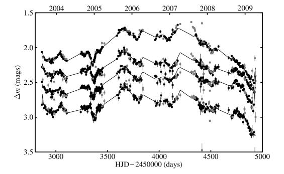
We modeled $\zeta_{i}(t)$ for images A, C, and D as linear functions of time (image B was used as the reference image). For each (non-reference) image, the curve was parameterized by $\zeta_{i}(t)=b_{0i}+b_{1i}\hat{t}$, where $\hat{t}$ is again defined as a scaled time variable running from $-1$ at the beginning of the light curve to $1$ at its end. This choice allowed us to test for the presence of a $d\ln{M}/d\ln{A}$ term even in the presence of contamination of the quasar light curves because the contamination $C$ should not vary with time. The source light curve and microlensing curves were modeled as polynomials of order $N_{\mathrm{src}}=120$ and $N_{\mu}=4$, respectively. Including $\zeta(t)$ dramatically improves the fit to the data from $\chi^{2}=2036$ for $N_{\mathrm{dof}}=1190$ to $\chi^{2}=1699$ for $N_{\mathrm{dof}}=1184$. We show the best-fit model light curves along with the data in Figure 5, and the best-fit parameters for the $\zeta_{i}(t)$ curves in Table 2. The best-fit time delays are the same within the errors whether or not $\zeta(t)$ is included, and are broadly consistent with those reported by Kochanek et al. (2006), in the sense that the order of arrival is preserved. In detail, our best-fit time delays differ from those previously reported by $\sim 1$ to $4\sigma$ (though correlations between the measured values reduce this tension). The discrepancy is due to our strategy of modeling the microlensing as a single polynomial spanning all six seasons, instead of a separate polynomial for each season, as was done in the earlier work. When we fit each season separately, we recovered time delays within $1\sigma$ of the previously reported values. Increasing $N_{\mu}$ improves the agreement between our delays and the reported delays, but the improvement is rather slow; our tests required $N_{\mu}\sim 20$ before the discrepancy was cut in half. It is not our present goal to recalculate the time delays, but we discuss in Section 6 some potential implications of our analysis for time delay estimates. We performed a second fit, holding the time delays constant at the previously reported values, and found that the $\chi^{2}/N_{\mathrm{dof}}$ increased to $1750/1187$, while the best-fit $\zeta(t)$ parameters were virtually unchanged. We report them in Table 2.

The significantly non-zero linear coefficient $b_{1}$ in the best-fit $\zeta_{i}(t)$ curves for image A (see Table 2) suggests that the changing accretion disk size has an appreciable effect on at least that image’s light curve. It is worth noting that this image was already thought to be affected by microlensing (Kochanek et al., 2006). However, the limitations associated with our analysis method prevent us from placing too much quantitative confidence in this result. The fit requires that the microlensing variability, as well as the variation in $\zeta(t)$, be slow in time. It also did not give sensible results when we attempted to fit individual seasons because of instabilities between the microlensing terms $\Delta\mu$ and $\zeta(t)$. Finally, it takes no account of the correlation between the microlensing caustic pattern and its derivative with respect to source size — the microlensing terms and the $\zeta(t)$ terms were fit independently. Because of these limitations, and because we have analyzed only a single lensed quasar without carefully addressing the problem of contaminating light, we cannot yet comment on the value of $\epsilon$ in detail.

The Bayesian Monte Carlo analysis method described by Kochanek (2004) and updated to include stellar motions by Poindexter & Kochanek (2010b) addresses most of these limitations. This method simulates microlensing light curves using the same technique as described in Section 3, but on a much larger scale. Simulated light curves that are found to be consistent with the measured data contribute to a Bayesian determination of parameters such as the source size and average microlens mass. The $\epsilon$ parameter may be added to the analysis as an additional parameter, and the source size allowed to vary with time when the light curves are simulated. This treatment allows for arbitrary microlensing variability, and would treat the $d\ln{M}/d\ln{A}$ terms self-consistently. We are optimistic that this improved analysis, applied to a number of light curves, will allow constraints to be placed on $\epsilon$.

Table 2HE 0435$-$1223 best-fit $\zeta(t)$ parameters

	Fixed delays		Free delays
	$b_{0}$	$b_{1}$	$b_{0}$	$b_{1}$
A	$0.92^{{}_{+.04}}_{{}^{-.03}}$	$-0.45^{{}_{+.07}}_{{}^{-.06}}$	$0.93^{{}_{+.03}}_{{}^{-.04}}$	$-0.43^{{}_{+.06}}_{{}^{-.07}}$
B	$\equiv 1$	$\equiv 0$	$\equiv 1$	$\equiv 0$
C	$0.98^{{}_{+.05}}_{{}^{-.03}}$	$\mbox{$\phantom{-}$}0.11^{{}_{+.10}}_{{}^{-.07}}$	$1.00^{{}_{+.04}}_{{}^{-.04}}$	$\mbox{$\phantom{-}$}0.12^{{}_{+.09}}_{{}^{-.08}}$
D	$1.15^{{}_{+.06}}_{{}^{-.04}}$	$-0.10^{{}_{+.11}}_{{}^{-.09}}$	$1.16^{{}_{+.05}}_{{}^{-.05}}$	$-0.08^{{}_{+.09}}_{{}^{-.10}}$
$\chi^{2}/N_{\mathrm{dof}}$	$1750/1187$		$1699/1184$

Note. — Errors represent formal 95% ($\Delta\chi^{2}=4$) confidence intervals. Because image B was the reference image, its parameters were fixed at the nominal values.

6. Conclusions

We have described a new effect arising from the microlensing of quasar accretion disks whose sizes vary in time. Assuming the change in size is proportional to some power of the change in luminosity of the quasar, we have derived what the effect would be on the light curves of lensed quasar images (see, e.g., Equation 6). The effect arises from the dependence of the microlensing magnification on the area of the source. This logarithmic derivative, $d\ln{M}/d\ln{A}$, depends on the macro-magnification of the image, the surface density of microlens stars, and the size of the source, along with the detailed arrangement of the microlensing caustic pattern. We have constructed probability distributions for the value of $d\ln{M}/d\ln{A}$ for various parameter combinations, and find that its value can be significantly nonzero. In particular, we note that it does not decrease in magnitude with increasing source size as strongly as the microlensing magnification itself does. We have also checked our mathematical model by constructing simulated light curves which demonstrate the microlensing of a time-varying disk.

We have demonstrated how fits may be made to such light curves to recover $\zeta(t)$, defined as the difference in $d\ln{M}/d\ln{A}$ between pairs of images. Some systematic errors are introduced by the presence of contaminating flux in the light curves, and we have discussed how these may be controlled. Applying the fitting method to the light curves of the four images of the lensed quasar HE 0435$-$1223, we find evidence for significant variation in this difference for image A relative to image B, indicating that the effect is likely occurring for this image. However, limitations of this fitting method, in particular the inconsistent treatment of the correlation between the microlensing and its size derivative, prevent us from saying anything quantitative. We propose, but have not implemented, an improved treatment based on the Bayesian Monte Carlo method of Kochanek (2004). This method is fully self-consistent, and ought to be more robust. The one limitation of this approach is that an a priori model of the source variability will have to be used to control the source size rather than the best fit estimate of the source light curve generated for each trial. A determination of $\zeta(t)$, in particular for a large sample of lensed quasar images, may be used to test the power-law slope of the dependence of quasar luminosity on disk size, a quantity that is predicted to be unity for simple blackbody disk models.

Our estimates of the time delays of HE 0435$-$1223 are only roughly consistent with those of Kochanek et al. (2006), whether or not we include the effect of $\zeta(t)$. Attempts to use the time delays of lensed quasar images for precision cosmology have often been hampered by a lack of robustness in measured delays, though the more serious problem remains model degeneracies (see discussion in Kochanek, 2006). In our case the tension is at least partially due to our choice of a low-order polynomial stretching across the entire 6-year light curve to model the microlensing variability. Although it was necessary for the sake of numerical stability, this model lacks the freedom necessary to describe the highest-frequency microlensing structures. This is another reason to adopt the self-consistent method described above. It is possible that previously unmodeled variable source size effects are also behind some of the discrepancy, in which case including the $\zeta(t)$ term would result in more accurate delay estimates. However, we note that we did not find significant differences in the best-fit time delays of HE 0435$-$1223 when the $\zeta(t)$ terms were allowed to vary versus when they were fixed at nominal values, nor did the best-fit $\zeta(t)$ terms change when the time delays were fixed at the previously reported values, so this remains speculation at best.

References

- Anguita et al. (2008) Anguita, T., Faure, C., Yonehara, A., Wambsganss, J., Kneib, J., Covone, G., & Alloin, D. 2008, A&A, 481, 615
- Bate et al. (2008) Bate, N. F., Floyd, D. J. E., Webster, R. L., & Wyithe, J. S. B. 2008, MNRAS, 391, 1955
- Blaes (2007) Blaes, O. 2007, in ASP Conf. Ser. 373, The Central Engine of Active Galactic Nuclei, ed. L. C. Ho & J.-W. Wang, 75
- Chartas et al. (2009) Chartas, G., Kochanek, C. S., Dai, X., Poindexter, S., & Garmire, G. 2009, ApJ, 693, 174
- Congdon et al. (2007) Congdon, A. B., Keeton, C. R., & Osmer, S. J. 2007, MNRAS, 376, 263
- Dai et al. (2010) Dai, X., Kochanek, C. S., Chartas, G., Kozłowski, S., Morgan, C. W., Garmire, G., & Agol, E. 2010, ApJ, 709, 278
- DePoy et al. (2003) DePoy, D. L., et al. 2003, in SPIE Conf. Ser. 4841, Instrument Design and Performance for Optical/Infrared Ground-based Telescopes, ed. M. Iye & A. F. M. Moorwood, 827
- Eigenbrod et al. (2008) Eigenbrod, A., Courbin, F., Meylan, G., Agol, E., Anguita, T., Schmidt, R. W., & Wambsganss, J. 2008, A&A, 490, 933
- Floyd et al. (2009) Floyd, D. J. E., Bate, N. F., & Webster, R. L. 2009, MNRAS, 398, 233
- Gould & Miralda-Escude (1997) Gould, A. & Miralda-Escude, J. 1997, ApJ, 483, L13
- Kelly et al. (2009) Kelly, B. C., Bechtold, J., & Siemiginowska, A. 2009, ApJ, 698, 895
- Kochanek (2004) Kochanek, C. S. 2004, ApJ, 605, 58
- Kochanek (2006) Kochanek, C. S. 2006, in Gravitational Lensing: Strong, Weak, and Micro, ed. G. Meylan, P. North, & P. Jetzer (Berlin: Springer), 91
- Kochanek et al. (2006) Kochanek, C. S., Morgan, N. D., Falco, E. E., McLeod, B. A., Winn, J. N., Dembicky, J., & Ketzeback, B. 2006, ApJ, 640, 47
- Kozłowski et al. (2010) Kozłowski, S., et al. 2010, ApJ, 708, 927
- Kroupa (2001) Kroupa, P. 2001, MNRAS, 322, 231
- Kundic et al. (1997) Kundic, T., et al. 1997, ApJ, 482, 75
- MacLeod et al. (2010) MacLeod, C. L., et al. 2010, ApJ, 721, 1014
- Morgan et al. (2010) Morgan, C. W., Kochanek, C. S., Morgan, N. D., & Falco, E. E. 2010, ApJ, 712, 1129
- Mortonson et al. (2005) Mortonson, M. J., Schechter, P. L., & Wambsganss, J. 2005, ApJ, 628, 594
- Mosquera et al. (2009) Mosquera, A. M., Muñoz, J. A., & Mediavilla, E. 2009, ApJ, 691, 1292
- Poindexter & Kochanek (2010a) Poindexter, S. & Kochanek, C. S. 2010a, ApJ, 712, 668
- Poindexter & Kochanek (2010b) Poindexter, S. & Kochanek, C. S. 2010b, ApJ, 712, 658
- Poindexter et al. (2008) Poindexter, S., Morgan, N., & Kochanek, C. S. 2008, ApJ, 673, 34
- Pooley et al. (2007) Pooley, D., Blackburne, J. A., Rappaport, S., & Schechter, P. L. 2007, ApJ, 661, 19
- Pooley et al. (2009) Pooley, D., Rappaport, S., Blackburne, J., Schechter, P. L., Schwab, J., & Wambsganss, J. 2009, ApJ, 697, 1892
- Schechter et al. (2003) Schechter, P. L., et al. 2003, ApJ, 584, 657
- Schild (1996) Schild, R. E. 1996, ApJ, 464, 125
- Wambsganss (2006) Wambsganss, J. 2006, in Gravitational Lensing: Strong, Weak, and Micro, ed. G. Meylan, P. North, & P. Jetzer (Berlin: Springer), 453
- Wambsganss et al. (1990) Wambsganss, J., Paczynski, B., & Katz, N. 1990, ApJ, 352, 407
- Wyithe & Loeb (2002) Wyithe, J. S. B. & Loeb, A. 2002, ApJ, 577, 615