Selective Call Out and Real Time Bidding

Abstract

Ads on the Internet are increasingly sold via ad exchanges such as RightMedia, AdECN and Doubleclick Ad Exchange. These exchanges allow real-time bidding, that is, each time the publisher contacts the exchange, the exchange “calls out” to solicit bids from ad networks. This aspect of soliciting bids introduces a novel aspect, in contrast to existing literature.

This suggests developing a joint optimization framework which optimizes over the allocation and well as solicitation. We model this selective call out as an online recurrent Bayesian decision framework with bandwidth type constraints. We obtain natural algorithms with bounded performance guarantees for several natural optimization criteria. We show that these results hold under different call out constraint models, and different arrival processes. Interestingly, the paper shows that under MHR assumptions, the expected revenue of generalized second price auction with reserve is constant factor of the expected welfare. Also the analysis herein allow us prove adaptivity gap type results for the adwords problem.

1 Introduction

A dominant form of advertising on the Internet involves display ads; these are images, videos and other ad forms that are shown on a web page when viewers navigate to it. Each such showing is called an impression. Increasingly, display ads are being sold through exchanges such as RightMedia, AdECN and DoubleClick Ad Exchange. On the arrival of an impression, the exchange solicits bids and runs an auction on that particular impression. This allows real time bidding where ad networks can determine their bids for each impression individually in real time (for an example, see [24]), and more importantly where the creative (advertisement) can be potentially produced on-the-fly to achieve better targeting [22].

This potential targeting comes hand in hand with several challenges. The Exchange and the networks face a mismatch in infrastructure and capacities and objectives. From an infrastructure standpoint, the volume of impressions that come to the exchange is very large comparison to a smaller ad network limited in servers, bandwidths, geographic location preferences. This implies a bound on the number of auctions the network can participate in effectively. A network would prefer to be solicited only on impressions which are of interest to it, and in practice use a descriptive languages to specify features of impressions (say, only impressions from NY). However this is an offline feature and runs counter to the attractiveness of real time bidding. Therefore the exchange has to “call out” to the networks selectively, simultaneously trying to balance the objective of soliciting as many networks as possible and increasing total value, as well as not creating congestion or situations where solicitations are not answered.

This leads to a host of interesting questions in developing a joint optimization framework that optimizes over the allocation objective as well as the decisions to solicit the bids. Specifically, a participant would be solicited for only a predetermined fraction of impressions. Moreover, these solicitations, referred to as “call outs” henceforth, need to be performed in a smooth manner and avoid burstiness. The impressions need to be managed in an online manner, which suggests the use of online algorithms. The burstiness properties suggests using a queueing model. And the overall goal is to optimize objectives such as (expected) welfare, revenue. While each of these issues have been considered in isolation, the overall challenge is to develop a joint framework, which in turn raises interesting questions about the interactions between different parts of the framework.

The call out framework is formally modeled in Section 1.1. The online allocation aspect, with a view that the call out constraints acts as budgets, is reminiscent of the online ad allocation framework for search ads, or the Adwords problem [19, 5, 7], and its stochastic variants [9, 27]. However the call out framework is significantly different, which we discuss below.

The Adwords problem is posed in the deterministic setting where the expected revenue is treated as a known deterministic reward of allocating an impression $j$ to an advertiser $i$. The call out framework has no deterministic analogue; the rationale of the exchange is that the bids are not known. If the bids were known (or internal) then we would only call out the winners (assuming multiple slots) of the auction, which is the path taken by the Adwords problem. The call-out framework is similar to Bayesian mechanism design [21]. This has some fairly broad conceptual implications.

First, is the notion of “adaptivity gap”, where a policy is allowed to react to realization of the random variables. The analysis of adaptivity gap is the central question in the exchange setting. This is also relevant in the context of search ads and the adwords setting where the revenue is achieved on a click which is a random event. The adwords model uses the deterministic expectation but it is reasonable to allow an algorithm to adapt to this event (consider low click through rates and large bids, such that a payout affects the budget substantially). To the best of our knowledge, no analysis of adaptivity gap exists for the adwords problem but such a result will follow from our analysis. In the call out setting, when optimizing for welfare or total value, the assignment occurs after the bids are obtained, which has considerable gap in comparison to the assignment that assigns before obtaining the realizations (reduces to the expectations).

Second, many objective functions such as generalized second price with reserve (henceforth GSP-Reserve), for one or multiple slots, have a very different behavior in the Bayesian and deterministic settings. The gap between assignment after and before the realizations is more stark in this context – consider running Myerson’s (or similar) mechanism on the expected bids instead of the distributions. Note that in GSP-Reserve we announce an uniform reserve price, before the bids are solicited as in [21]. For known deterministic bids, reserve prices can be made equal to the bid, and are not useful. Strong lower bounds hold for GSP without reserves [1].

Third, the notion of a comparison class in case of call out optimization framework requires more care. In the setting of these large exchanges, a comparison class with full foreknowledge of all information (in particular, the realization of the bids) is unrealistic. Moreover, the realizations of the bids depends on the networks which are called out, and two different strategies that call out to two different subsets will have completely different information. Thus to compare two algorithms, it appears that we should compare their expected outcome – but each algorithm is allowed to be adaptive. Thus a combination of stochastic and online models are in order in this setting.

This combination of stochastic and online models relates the call out framework to the stochastic variants of the Adwords problem [9, 27]. But while the similarity implies that Lagrangian decoupling techniques for separable convex optimization pioneered by Rockafellar [25] apply, the different possible objectives of the call-out framework are not convex. In fact, in the case of optimizing revenue in GSP (with reserve) or in posted price mechanisms, the objective is not submodular for all prices (as in welfare maximization). Submodular maximization with linear constraints has been studied, and while good approximation algorithms exist [6, 17], they are inherently offline – the key aspect of call out optimization is that the decision has to be made in an online fashion. The same is true for sequential posted price mechanisms analyzed in [8, 4] (albeit with more general matroid setting), the posted prices in the call out setting need to be announced in parallel (and the eventual allocation is sequential). Other than formulating the call out framework, significant contribution of this paper is to demonstrate that relaxations of natural objective functions can be made separable (as in [25]), yet with bounded loss in performance ratio. Subsequent to the formulation, standard techniques of online stochastic optimization can be applied.

1.1 Selective Call Out: The Model

Let $n$ be the number of ad networks $1,2\ldots n$. We assume that impressions arrive from a fixed (unknown) distribution over a finite set $U_{I}$, and that there exists a finite set of bid values $U_{B}$, where $L=\max\{u|\ u\in U_{B}\}$. In the following, ad networks will be indexed by $i\in\{1,2\ldots n\}$, impressions by $j\in U_{I}$ and bid values by $k\in U_{B}$. The problem setting involves several steps:

1. An impression (or keyword) $j$, assumed drawn from a distribution $\mathcal{D}$, comes to the exchange. There may be multiple slots associated with a single impression, corresponds to text ads being blocked together, different locations in the page, which are often characterized by different discount rate. Let there be $M$ slots, with discount rates $1\geq\varrho_{1}\geq\varrho_{2}\ldots\geq\varrho_{M}\geq 0$. If a bidder bids $v$, then it is assumed that the bid for the $\ell^{th}$ slot is $v\varrho_{\ell}$. The case of $M=1$ is common and correspond to a basic pay-per-impression mechanism with discount rate $1$. All subsequent discussions apply to this common case as well.

2. Given an impression $j$, the bid of ad network $i$ for impression $j$ is drawn from a fixed distribution $\mathbf{V}_{ij}$ such that the bid is $v$ with probability $p_{ijv}$. Note that the bids of different networks are likely to be correlated based on the perceived value of the impression, however, conditioned on $j$, the specific dynamics of different bidders can be construed to be independent. We assume that the exchange has learned or can predict these $p_{ijv}$ given the impression $j$. This is an assumption similar to estimation processes used by search engines to predict the value of different advertisements (albeit under static standing bids).

3. The exchange decides on the subset $S_{j}$ of networks to call out, subject to the Call-Out constraints, which roughly bounds the rate at which the exchange can send impressions to solicit bid from an ad network. This decision is executed before seeing the next impression.

To define a specific problem in the above framework, we need to specify (i) an objective function (ii) a model for call out constraints, and (iii) the comparison class. The goal is to design a call-out policy that satisfies (ii) and is near optimal in the objective function (i), when compared to other algorithms in class (iii). We discuss the instantiations of (i),(ii), and (iii) in the following.

(i) Objective Functions. We consider three different objective functions. (a) Total Value: The sum of the maximum bids in $S_{j}$ over the arriving impressions $j$. (b) GSP-Reserve (defined above) and (c) Revenue under posted price mechanism (take-it-or-leave-it prices). All the quantities are in expectation. Total value corresponds to the welfare. The GSP with an uniform reserve price is a common mechanism used in these settings. Posted Prices (different networks may get different prices) are also used in this context. Note that the mechanism is parallel posted price because the prices are posted before any bids are obtained, and not sequential as in [8, 4].

(ii) Call Out Constraint Models. The simplest model for the call out constraints is a model where one impression arrives at the exchange at each time step and if the total number of arrivals is $m$, ad network $i$ can be solicited at most times for some known $\rho_{i}\leq 1$. We will refer to this as time average model under uniform arrival – which describes the constraints at the outgoing and incoming sides of the exchange respectively. Most of the paper will focus on this model – primarily because we can show that other common models reduce to this variant. The non-initiated reader can skip the description of these models and proceed to (iii).

On the incoming side of the exchange, standard practice is to assume bursty (Poisson) arrivals. We consider this generalization. On the outgoing side, the simple model allow the possibility that the call-outs to a network are made on contiguous subset of impressions. This misses the original goal that the ad network would receive the impressions at a “smooth” rate. A common model used for behavior is the token bucket model [26]. A token bucket has two parameters, bucket size $\sigma$ and token generation rate $\rho$. The tokens represent sending rights, and the bucket size is the maximum number of tokes we can store. The tokens are generated at a rate of $\rho$ per unit time, but the number of tokens never exceeds $\sigma$. In order to send, one needs to use a token, and if there are no tokens, one can not send. The output stream of a $(\sigma,\rho)$ token bucket can be handled by a buffer of size $\sigma$ and a time average rate of $\rho$ – the buffer is initially full. Unlimited buffer size corresponds to the time average model.

(iii) Comparison Class. Given the call out constraints, we define the class of admissible policies.

Definition 1

An admissible call out policy specifies (possibly with randomization), for each arriving impression $j$, the subset $S_{j}$ of ad networks to call out, while satisfying all call out constraints over the entire sequence of impressions. The policy bases its decision on the prior information about the bid distributions, and has no knowledge of the actual bid values. In the case of GSP-Reserve mechanism, the call out policy also decides the reserve price for each impression. In the case of a posted price mechanism, the call out policy also decides the posted/take-it-or-leave-it prices.

Our comparison class is the set of all admissible call out policies which know the bid distributions for every impression, but do not know the actual realization of the bids. The performance of a policy is measured as the expected (over the bid distributions and the impression arrivals) objective value obtained per arriving impression, when impressions are drawn from $\mathcal{D}$.

1.2 Our Results, Roadmap and Other related Work

We provide three algorithms LP-Val, LP-GSP, and LP-Post for the three objectives discussed for the time average uniform arrival model. We then prove that any approximation for any additive objective function translates naturally to an approximation for the other constraint models. Recall, $L$ is the largest possible bid. A policy is $\alpha$-approximate if it achieves at least $\alpha$ times the performance of the optimal policy for the corresponding objective. The algorithms will have a natural two-phase approach where we use the $t$ initial impressions as a sample as exploration and subsequently use/exploit this algorithm (see Section 2 for more discussion). We show that:

Theorem 1

Suppose the optimal policy has expected total value at least $\delta>0$. For any $\epsilon>0$, LP-Val with a sample of $t=\tilde{O}(\frac{n^{2}L}{\delta\epsilon})$ impressions gives a $(1-\frac{1}{e}-\epsilon)$-approximate policy.

Theorem 2

Suppose the optimal GSP-Reserve policy has expected revenue at least $\delta>0$. For any $\epsilon>0$, LP-GSP with a sample of $t=\tilde{O}(\frac{n^{2}L}{\delta\epsilon})$ impressions gives a $O(1)$-approximate policy, if all bid distributions satisfy the monotone hazard rate (MHR) property. Moreover, the call outs of the policy derived from LP-GSP are identical to those of the policy derived from LP-Val.

In particular, we show that when every bidder is solicited – GSP-Reserve achieves a revenue that is $O(1)$ factor of optimal welfare, when all bid distributions satisfy the MHR property. This is a common distributional assumption in economic theory, and is satisfied by many distributions [3]. This result is in the same spirit as (but immediately incomparable to) the result in [4], which relates the optimum sequential posted price revenue to the optimal welfare under the same assumptions. We are unaware of such results about GSP-Reserve.

Theorem 3

Suppose the optimal posted price policy has expected revenue at least $\delta>0$. For any $\epsilon>0$, LP-Post with a sample of $t=\tilde{O}(\frac{n^{2}L}{\delta\epsilon})$ impressions gives a $(1-\frac{1}{e}-\epsilon)$-approximate policy.

We do not need the MHR assumption unlike the result in [4] for sequential posted prices, since the comparison classes are different (and the prices are posted in parallel). We next show that:

Theorem 4

For a given distribution on impressions $\mathcal{D}$, suppose we have an $\alpha$-approximate policy for an objective which is additive given the allocations and the realizations (and is at least $\delta>0$) in the time average uniform arrival call out model. Let $\sigma_{i}>\sigma\ \forall i$. Then we can convert the policy to a $(\alpha-\frac{1}{\sigma-1})$-approximate policy in the token bucket model. The result extends to Poisson arrivals.

Roadmap: We summarize the results on online stochastic convex optimization in Section 2. We subsequently discuss the the total value problem in Section 3. We discuss the GSP-Reserve problem in Section 4. The posted price problem is discussed in Section 5. The token bucket model and other arrival assumptions are discussed in Section 6. To draw a contrast to the stochastic results, the adversarial order setting is discussed in Appendix A.

Other Related Work: A combination of stochastic and online components appear in many different settings [14, 15, 2, 13] which are not immediately relevant to the call-out problem. We note that the bandwidth-like constraints (where the constraint is on a parameter different than the obtained value, as is the case for call-outs) has not studied in the bandit setting (see [16, 23]) because the horizon is constrained. Finally, bidding and inventory optimization problems studied in the context of ad exchanges [11, 10, 20], are not related to the call out optimization problems.

2 Preliminaries

Consider a maximizing a “separable” linear program (LP) ${\cal L}$ defined on $Q$ global constraints with right hand side $b_{i}$, such that the Lagrangian relaxation produced by the transferring these constraints to the objective function decouples into a collection of independent non-negative smaller LPs ${\cal L}_{j}$ over $n^{\prime}$ variables and local constraints. This implies that the objective function of ${\cal L}$ is a weighted linear combination of ${\cal L}_{j}$. The uniqueness of the optimum solutions for ${\cal L}_{j}$ implies that ${\cal L}$ reduces to finding the Lagrangian multipliers. The unique solution is achieved by adding “small perturbations”, see Rockafellar [25]. However, this approach only provides a certificate of optimality and a solution, once we are given the Lagrangians. The approach does not give us an algorithm to find the Lagrangian multipliers themselves.

Devanur and Hayes [9] showed that if the smaller LPs could be sampled with the same probability as their contribution to the objective of ${\cal L}$, and the derivatives of the Lagrangian can be bounded, then the Lagrangians derived from a small number of samples (suitably scaled) can be used to solve the overall LP. The weighted sampling reduces to the prefix of the input if the ${\cal L}_{j}$s arrive in random order (see [12]). This was extended to convex programs in [27]. The number of sample bound requires several (easy) Lipschitz type properties:

1. The optimum value of ${\cal L}$ is at least $\delta>0$ and the optimum solution of ${\cal L}_{j}$ is at most $R$.

2. For each setting of the Lagrangians, every ${\cal L}_{j}$ has a unique optimum solution.

3. Reducing $b_{i}$ by a factor of $1-\epsilon$ does not reduce ${\cal L}$ by more than a factor of $(1-\epsilon)$.

4. ${\cal L}$ does not change by more than a constant times $1+\epsilon$ if we alter the value of the optimum Lagrangian multipliers by a factor of $1+\epsilon$.

Theorem 5

Sample $t=\tilde{O}(\frac{n^{\prime}QR}{\delta\epsilon})$ of the smaller linear programs and consider the linear program ${\cal L^{\prime}}$ which corresponds to the union of these smaller linear programs and suitably scaled global constraints. If we use the optimum Lagrangian multipliers corresponding to the global constraints of ${\cal L^{\prime}}$ to solve the decoupled instances of ${\cal L}_{j}$ as they are available (in an online fashion) then we produce a $1+\epsilon$ approximation to the optimum solution of ${\cal L}$.

In the setting of Adwords, the smaller LPs correspond to the arrival of an impression, and the associated assignment. Thus the stochastic framework of the Adwords problem is obviously of relevance to the call out optimization framework. However the focus shifts on solving the smaller LPs which encode the call out decision. A nice outcome of the approach is a simple two phase algorithm; an Exploration phase where the samples are drawn, and an Exploitation phase where the Lagrangian multipliers are used. If $Q,n^{\prime},R$ are small, then the exploration phase can be (relatively) short and this yields a natural algorithm. Thus the goal of the rest of the paper would be to formulate separable convex relaxations and achieve the mentioned properties.

3 The Total Value Problem

In this section, we prove Theorem 1, and describe LP-Val. Let $q_{j}$ denote the probability that impression $j$ arrives. We shall add infinitesimal random perturbations to $p_{ijv}$ which shall not affect the performance of any policy but ensure $p_{ijv}$ are in general positions, that is, any combination of them will almost surely create a non-singular matrix.

The LP Relaxation:

1. Let $x_{ij}$ be the (conditional) probability that advertiser $i$ was called out on impression $j$.

2. Let $y_{ijv\ell}$ be the probability that advertiser $i$ bid the value $t$ and was assigned the slot $\ell$ (also conditioned on $j$). The constraints are named as $A(x,y)$ and $B(x,y)$ as shown.

$$LP1= \max \sum_{j}q_{j}\sum_{v}\sum_{i}\sum_{\ell}v\varrho_{\ell}y_{ijv\ell}\quad\mbox{s.t.}\begin{array}[]{l}\quad\sum_{j}q_{j}x_{ij}\quad\leq\rho_{i}\\ \left.\begin{array}[]{ll}\sum_{i}\sum_{v}y_{ijv\ell}\leq 1\\ \left.\begin{array}[]{ll}x_{ij}&\leq 1\\ \sum_{\ell}y_{ijv\ell}&\leq p_{ijv}x_{ij}\\ x_{ij},y_{ijv\ell}&\geq 0\end{array}\right\}B(x,y)\end{array}\right\}A(x,y)\end{array}$$

Decoupling: Let $\lambda^{*}_{i}$ be the optimum Lagrangian variable for the constraint $\sum_{j}q_{j}x_{ij}\leq\rho_{i}$. $LP1$ then decouples to smaller LPs, $LP2(j,\vec{\lambda^{*}_{i}})$ subject to the constraints $A(x,y)$.

$$LP1=LP1(\vec{\lambda^{*}_{i}}) = \sum_{i}\lambda^{*}_{i}\rho_{i}+\sum_{j}q_{j}LP2(j,\vec{\lambda^{*}_{i}})\quad\mbox{where}\quad LP2(j,\vec{\lambda^{*}_{i}})=\max\left(\sum_{v}\sum_{i}\sum_{\ell}v\varrho_{\ell}y_{ijv\ell}-\sum_{i}\lambda^{*}_{i}x_{ij}\right)$$

Solving $\mathbf{LP2(j,\vec{\lambda^{*}_{i}})}$. We begin by considering the dual. Let $\tau_{j\ell}$ be the dual of the constraint $\sum_{i}\sum_{v}y_{ijv\ell}\leq 1$. Let $\xi_{ijv}$ correspond to the dual of the constraint $\sum_{\ell}y_{ijv\ell}\leq p_{ijv}x_{ij}$. Let $\zeta_{ij}$ correspond to the dual of $x_{ij}\leq 1$.

$$DualLP2(j,\vec{\lambda^{*}_{i}}) = \min\sum_{i}\zeta_{ij}+\sum_{\ell}\tau_{j\ell}\quad\mbox{s.t.}\quad\begin{array}[]{ll}\tau_{j\ell}+\xi_{ijv}&\geq v\varrho_{\ell}\\ \zeta_{ij}-\sum_{v}\xi_{ijv}p_{ijv}&\geq-\lambda^{*}_{i}\\ \tau_{j\ell},\xi_{ijv},\zeta_{ij}&\geq 0\end{array}$$

Lemma 3.1

Let $\tau^{*}_{j\ell}$ be the optimum dual variables for $LP2$. Then (i) For all $\ell$ there exists $i$ and $v\geq\tau^{*}_{j\ell}/\varrho_{\ell}$ such that $\xi^{*}_{ijv}=v\varrho_{\ell}-\tau^{*}_{j\ell}$. (ii) $\tau^{*}_{j\ell}/\varrho_{\ell}$ is non-increasing in $\ell$.

Proof: For every $\ell$ there must be some $i,v$ such that we have $\tau^{*}_{j\ell}+\xi^{*}_{ijv}=v\varrho_{\ell}$. Otherwise we can keep decreasing $\tau^{*}_{j\ell}$, keeping all other variables the same and contradict the optimality of the dual solution. Now $\xi^{*}_{ijv}\geq 0$ and the condition on $t$ follows. The condition corresponds to the set of points $(v,\xi^{*}_{ijv})$ in the two dimensional $(x,y)$ plane being above the lines $\{y=\varrho_{\ell}x-\tau^{*}_{j\ell}\}$.

For the second part, consider $\tau^{*}_{j\ell}$ and the $i,v$ such that we have $\tau^{*}_{j\ell}+\xi^{*}_{ijv}=v\varrho_{\ell}$. Define $t$ to be the support of $\ell$. Let $v\geq\tau^{*}_{j\ell}/\varrho_{\ell}$ be the largest such support of $\ell$. Consider $\tau^{*}_{j(\ell-1)}$. We have $(\tau^{*}_{j(\ell-1)}+\xi^{*}_{ijv})/\varrho_{\ell-1}\geq v=(\tau^{*}_{j\ell}+\xi^{*}_{ijv})/\varrho_{\ell}$. But $\varrho_{\ell-1}\geq\varrho_{\ell}$ and thus $\tau^{*}_{j\ell}/\varrho_{\ell}$ are non-increasing in $\ell$. Moreover, if $\varrho_{\ell}=\varrho_{\ell-1}$ then $\tau^{*}_{j\ell}=\tau^{*}_{j(\ell-1)}$ (starting from the support of $\ell-1$).      

Decoupling $\mathbf{LP2(j,\vec{\lambda^{*}_{i}})}$ itself. Consider $LP2(j,\vec{\lambda^{*}_{i}})$ with the Lagrangians $\tau^{*}_{j\ell}$. The problem decomposes under the constraints $B(x,y)$, to

$$LP2(j,\vec{\lambda^{*}_{i}}) = \sum_{\ell}\tau^{*}_{j\ell}+\sum_{i}LP3(j,\vec{\lambda^{*}_{i}},\vec{\tau^{*}_{j\ell}},i)\quad\mbox{where}\quad LP3(j,\vec{\lambda^{*}_{i}},\vec{\tau^{*}_{j\ell}},i)=\max\left(\sum_{\ell}\sum_{v}\left[v\varrho_{\ell}-\tau^{*}_{j\ell}\right]y_{ijv\ell}-\lambda^{*}_{i}x_{ij}\right)$$

Lemma 3.2

Define $\ell(v)=\arg\max_{\ell^{\prime}}\left\{\varrho_{\ell^{\prime}}v-\tau^{*}_{j\ell^{\prime}}|\varrho_{\ell^{\prime}}v>\tau^{*}_{j\ell^{\prime}}\right\}$ and $\ell(t)=M+1$ if the set is empty. Set $y^{*}_{ijv\ell}=p_{ijv}$ if $\ell=\ell(v)$ and $0$ otherwise. If $\sum_{v}\sum_{\ell}v\varrho_{\ell}y^{*}_{ijv\ell}\geq\lambda^{*}_{i}$ we set $x_{ij}=1$ and $y_{ijv\ell}=y^{*}_{ijv\ell}$. Otherwise we set $x_{ij}=y_{ijv\ell}=0$.

Proof: $LP3(j,\vec{\lambda^{*}_{i}},\vec{\tau^{*}_{j\ell}},i)$ is optimized at $x_{ij}=1$ or $x_{ij}=0$. This is because if $0<x_{ij}<1$ and $\sum_{\ell}\sum_{v}\left[v\varrho_{\ell}-\tau^{*}_{j\ell}\right]y_{ijv\ell}-\lambda^{*}_{i}x_{ij}>0$ then we can multiply all the variables by $1/x_{ij}$ and have a better solution. If the latter condition is not true then $x_{ij}=0$ is an equivalent solution. If $x_{ij}=1$ the optimal setting for $y_{ijv\ell}$ is $y^{*}_{ijv\ell}$. (Note that $y^{*}_{ijv\ell}$ is uniquely determined for a fixed $t$.) Thus the overall optimization follows from comparing the $x_{ij}=1$ and $x_{ij}=0$ case.      

Interpretation and the Call Out Algorithm: Given $\{\tau^{*}_{j\ell}\}^{M}_{\ell=1}$, the distribution $\{p_{ijv}\}$ for $i$, is divided into at most $M+1$ pieces (some of the pieces can be a single point) given by the upper envelope (the constraint max) of the lines $\{\varrho_{\ell}x-\tau^{*}_{j\ell}\}_{\ell=1}^{M}$ and the line $y=0$, in the $x$–$y$ coordinate plane. Intuitively, seeing the value $x=t$, if the upper envelope corresponds to the equation $\varrho_{\ell}x-\tau^{*}_{j\ell}$ then we are “interested” in the slot $\ell$. If the weighted (by $\varrho_{\ell}$) sum of interests, given by $\sum_{v}v\varrho_{\ell}y^{*}_{ijv\ell}$ exceeds $\lambda^{*}_{i}$, then it is beneficial to call out $i$. We call out based on this condition and allocate the slots in decreasing order of bids.

Analysis: The LP2 solution satisfies: $LP1=\sum_{i,v}vp_{ijv}\varrho_{\ell(v)}$ and $\sum_{i,v:\ell(v)=\ell}p_{ijv}=1$. For each slot $\ell$, let $w_{i}(\ell)=\sum_{v:\ell(v)=\ell}vp_{ijv}$ and $u_{i}(\ell)=\sum_{v:\ell(v)=\ell}p_{ijv}$. Order the $i$ in non-increasing order of $w_{i}(\ell)/u_{i}(\ell)$ inside the slot. If we call out to $i$ and get $t$, then for the sake of analysis we will consider its contribution to slot $\ell(t)$ only. Moreover, we stop the contribution to a slot $\ell$ if any any of the $i$ return a value $t$ with $\ell(t)=\ell$. The best $M$ ordered bids outperform the analyzed contribution in every scenario. Therefore it suffices to bound the contribution of the analysis.

Lemma 3.3

Suppose we are given a set of independent variables $Y_{i}$ such that $Pr[Y_{i}\neq 0]=u_{i}$ and $E[Y_{i}]=w_{i}$. Consider the random variable $Y$ corresponding to the process which orders the variables $\{Y_{i}\}$ in non-increasing order of $w_{i}/u_{i}$, and stops as soon as the first non-zero value is seen. Then $E[Y]=\sum_{i}\prod_{i^{\prime}<i}(1-u_{i^{\prime}})w_{i}\geq\sum_{i}w_{i}\left(1-e^{-1}\right)$.

Proof: Let $F(\{(w_{i},u_{i})\})=\sum_{i}\prod_{i^{\prime}<i}(1-u_{i^{\prime}})w_{i}$. Let $\lambda=\sum_{i}w_{i}/\sum_{i}u_{i}$. Given the sequence $\{(w_{i},u_{i})\}$ where $w_{i}/u_{i}$ are non-increasing, if there exists an $i$ such that $w_{i}/u_{i}\neq w_{i+1}/u_{i+1}$, then define a new sequence $\{(w^{\prime}_{i},u_{i})\}$ as follows:

$$w^{\prime}_{i^{\prime}}=\left\{\begin{array}[]{ll}w_{i^{\prime}}&\mbox{ if $i^{\prime}\neq i,i+1$}\\ w_{i}-\Delta&\mbox{ if $i^{\prime}=i$}\\ w_{i+1}+\Delta&\mbox{ if $i^{\prime}=i+1$}\end{array}\right.\quad\quad\mbox{where}\quad\quad\Delta=\frac{\frac{w_{i}}{u_{i}}-\frac{w_{i+1}}{u_{i+1}}}{\frac{1}{u_{i}}+\frac{1}{u_{i+1}}}$$

Note that $\sum_{i}w_{i}=\sum_{i}w^{\prime}_{i}$ and $w^{\prime}_{i}/u_{i}$ remains non-increasing. Now $F(\{(w_{i},u_{i})\})-F(\{(w^{\prime}_{i},u_{i})\})=\prod_{i^{\prime}<i}(1-u_{i^{\prime}})\Delta-\prod_{i^{\prime}<i+1}(1-u_{i^{\prime}})\Delta=\prod_{i^{\prime}<i}(1-u_{i^{\prime}})u_{i}\Delta>0$. Thus, we can repeatedly perform the above steps till we get a sequence such that $w^{\prime}_{i}/u_{i}$ remains the same for all $i$ and $\sum_{i}w_{i}=\sum_{i}w^{\prime}_{i}$. Clearly $w^{\prime}_{i}=\lambda u_{i}$ in this case. The function $F$ will continue to decrease, and

$$F(\{(w_{i},u_{i})\})\geq F(\{(w^{\prime}_{i},u_{i})\})=\sum_{i}\prod_{i^{\prime}<i}(1-u_{i^{\prime}})\lambda u_{i}=\lambda\left(1-\prod_{i}(1-u_{i})\right)\geq\lambda\left(1-e^{-\sum_{i}u_{i}}\right)$$

But $\frac{1}{x}(1-e^{-x})$ is decreasing over $[0,1]$ and the worst case is $x=1$.      

In slot $\ell$ (renumbering the advertisers in the order of $w_{i}(\ell)/u_{i}(\ell)$) we get an expected reward of $w_{i}(\ell)$ if we reach $i$. But the events are independent in a particular slot. Thus the expected reward in a slot is bounded by (using independence and Claim 3.3) to be $(1-e^{-1})$ times $\sum_{i}w_{i}(\ell)$. We now apply linearity of expectation across the slots – observe that the events across the slots are quite correlated. The expected reward is at least $(1-e^{-1})$ times $\sum_{\ell}\sum_{i}w_{i}(\ell)=LP1$. Theorem 1 follows from Lemmas 3.2 and 3.3 and the application of Theorem 5.

4 Generalized Second Price with reserve (GSP-Reserve)

The call outs for this problem would be exactly the same as the algorithm in Section 3. We will however adjust the reserve prices. The reserve price will be the same for all the advertisers being called out on that impression. In fact either we will run a single slot auction with a reserve price, or simply GSP for the $M$ slots. The decision will depend on the LP solution found for this specific impression (and the contributions of different parts of the LP). Recall that the bid distribution $\mathbf{V}_{ij}$ of advertiser $i$ on impression $j$ is assumed to satisfy the MHR property. We use the following:

Lemma 4.1

(Lemma 3.3 in [4]) For any random variable $V$ following an MHR distribution, let $v^{*}=\arg\min_{v}\{v|v\Pr[V\geq v]\geq\frac{1}{2}\sum_{v^{\prime}\geq v}v^{\prime}\Pr[V=v^{\prime}]\}$. Then $\Pr[V\geq v^{*}]\geq e^{-2}$.

The next lemma is a restatement of Lemma 3.2 and the subsequent analysis.

Lemma 4.2

Given an impression $j(t)$, and define $v_{1}(t)=\max_{\ell:\varrho_{1}\neq\varrho_{\ell}}(\tau^{*}_{j1}-\tau^{*}_{j\ell})/(\varrho_{1}-\varrho_{\ell})$. The call out to a set $S(t)\neq\emptyset$, ensures that $\sum_{i}\sum_{v\geq v_{1}(t)}p_{ijv}\geq 1$.

Definition 2

Given an impression $j(t)$, and the call out decision to a set $S(t)\neq\emptyset$ at time $t$, let $v^{*}_{m}(i,t)=\min\{v|2v\Pr[V_{ij}\geq v]\geq\sum_{v^{\prime}\geq v}v^{\prime}p_{ijv^{\prime}}\}$ and $\Psi(t)=\{i|i\in S(t)\mbox{ and }v_{1}(t)\leq v^{*}_{m}(i,t)\}$. Note that using Lemmas 4.1, and 4.2, we have $|\Psi(t)|\leq\lfloor e^{2}\rfloor=7$ since $i\in\Psi(t)$ contributes a probability mass of at least $e^{-2}$.

Lemma 4.3

Given an impression $j(t)$, and the call out decision to a set $S(t)\neq\emptyset$ at time $t$, we can set a single threshold $v^{*}(t)\geq v_{1}(t)$ such that if we set a reserve price $v^{*}(t)$ for a single slot then the revenue (ignoring the multiplicative discount factor $\varrho_{1}$) is at least $\frac{1}{4(7e^{2}+1)}\sum_{i\in S(t)}\sum_{v\geq v_{1}(t)}vp_{ijv}$.

Proof: Let $\sum_{i\in S(t)}\sum_{v\geq v_{1}(t)}vp_{ijv}=Z$. We have two cases, (i) $\sum_{i\in\Psi(t)}\sum_{v\geq v_{1}(t)}vp_{ijv}\geq 7e^{2}Z/(7e^{2}+1)$ or (ii) otherwise. In case (i), pick the $i\in\Psi(t)$ such that $\sum_{v\geq v_{1}(t)}vp_{ijv}$ is maximized, which is at least $e^{2}Z/(7e^{2}+1)$ since $|\Psi(t)|\leq 7$. Let $V_{ij}$ be the random variable that corresponds to the bid of advertiser $i$ on impression $j$. Now since $v^{*}_{m}(i,t)\geq v_{1}(t)$ we have that

$$\sum_{v\geq v^{*}_{m}(i,t)}vp_{ijv} \geq \Pr\left[V_{ij}\geq v^{*}_{m}(i,t)|V_{ij}\geq v_{1}(t)\right]\sum_{v\geq v_{1}(t)}vp_{ijv}\geq\Pr\left[V_{ij}\geq v^{*}_{m}(i,t)\right]\sum_{v\geq v_{1}(t)}vp_{ijv}\leq\frac{1}{e^{2}}\sum_{v\geq v_{1}(t)}vp_{ijv}$$

which is at least $Z/(7e^{2}+1)$. Now, if we set $v^{*}(t)=v^{*}_{m}(i,t)$ then just from $i$ we have $\sum_{i\in S(t)}\sum_{v\geq v^{*}(t)}p_{ijv}\geq\frac{1}{2}\sum_{v\geq v^{*}_{m}(i,t)}vp_{ijv}$ and therefore in this case the lemma is true.

In case (ii), we have $\sum_{i\in S(t)\setminus\Psi(t)}\sum_{v\geq v_{1}(t)}vp_{ijv}\geq Z/(7e^{2}+1)$. But for each $i\in S(t)\setminus\Psi(t)$ we have $v_{1}(t)\sum_{v\geq v_{1}(t)}p_{ijv}\geq\frac{1}{2}\sum_{v\geq v_{1}(t)}vp_{ijv}$ and as a consequence, $v_{1}(t)\sum_{i\in S(t)\setminus\Psi(t)}\sum_{v\geq v_{1}(t)}p_{ijv}$ is at least $Z/(2(7e^{2}+1))$. Consider setting $v^{*}(t)=v_{1}(t)$. Let $p=\sum_{i\in S(t)\setminus\Psi(t)}\sum_{v\geq v_{1}(t)}p_{ijv}$. Since $p\leq 1$ (from definition of $v_{1}(t)$, see Lemma 4.2) the probability of sale is at least $(1-\frac{1}{e})p$ which is bounded below by $p/2$. The Lemma follows in this case as well.      

Lemma 4.4

Given an impression $j(t)$, and the call out decision to a set $S(t)\neq\emptyset$ at time $t$, consider (i) If $\sum_{i\in S(t)}\sum_{v}v\varrho_{\ell(v)}y^{*}_{ijv\ell(v)}\geq 3\sum_{i\in S(t)}\sum_{v\geq v_{1}(t)}v\varrho_{1}y^{*}_{ijv1}$ then call-out to $S(t)$ and run regular GSP. (ii) Otherwise call-out to $S(t)$ and run a single slot auction with the threshold $v^{*}(t)$ given by Lemma 4.3. This algorithm gives a revenue which is $\Omega(1)$ factor of the LP bound on efficiency which is given by $\sum_{v}\sum_{i\in S(t)}\sum_{v}v\varrho_{\ell}y^{*}_{ijv\ell(v)}$. Note that the call out decisions are based on optimizing the total value/ efficiency of the slots, and thus are feasible.

Proof: Let the non-increasing ordered list of values that are returned for a time step be $a_{1}(t)$. Suppose we are in case (i). Then the revenue of GSP is at least $\sum_{r=1}^{M}\varrho_{r}a_{r+1}(t)$. Now since $\varrho_{r}$ are decreasing, and $a_{r}(t)$ are non-increasing,

$$\sum_{r=1}^{M}\varrho_{r}a_{r+1}(t)\geq\sum_{r=1}^{M}\varrho_{r}a_{r}(t)-\varrho_{1}a_{1}(t)\quad\quad\Longrightarrow\quad\text{\bf E}\left[\sum_{r=1}^{M}\varrho_{r}a_{r+1}(t)\right]\geq\text{\bf E}\left[\sum_{r=1}^{M}\varrho_{r}a_{r}(t)\right]-\varrho_{1}\text{\bf E}\left[a_{1}(t)\right]$$ (5)

We know from the rounding in Section 3 that $\text{\bf E}\left[\sum_{r=1}^{M}\varrho_{r}a_{r}(t)\right]\geq\left(1-\frac{1}{e}\right)\sum_{i\in S(t)}\sum_{v}v\varrho_{\ell}y^{*}_{ijv\ell(v)}$.

We observe that $\text{\bf E}\left[a_{1}(t)\right]\leq\sum_{i\in S(t)}\sum_{v\geq v_{1}(t)}vy^{*}_{ijv1}$. This is easily seen if we write an LP for the maximum value seen (this LP is for analysis only). Let $x_{iv}$ be the probability that $i\in S(t)$ is the maximum with value $v$. Then (we drop the index $j$ for convenience):

$$\text{\bf E}\left[a_{1}(t)\right] \leq LPMAX=\max\sum_{i}\sum_{v}vx_{iv}\quad\quad\mbox{s.t.}\quad\quad\begin{array}[]{lll}&&\sum_{i}\sum_{v}x_{iv}\leq 1\\ &&x_{iv}\leq p_{iv}\\ &&x_{iv}\geq 0\end{array}$$

The optimum solution of $LPMAX$ is $x^{*}_{iv}=p_{iv}$ for $v>\tau$ and $x^{*}_{iv}\leq p_{iv}$ for one $i$ and $v=\tau$. Here $\tau$ is the optimum dual variable for the constraint $\sum_{i\in S(t)}\sum_{v}x_{iv}\leq 1$. Note that $\sum_{i\in S(t)}\sum_{v}x^{*}_{iv}=1$.

For $v>v_{1}(t)$ we have $y^{*}_{ijv1}=p_{ijv}$ and $v<v_{1}(t)$ we have $y^{*}_{ijv1}=0$. Moreover $\sum_{i\in S(t)}\sum_{v\geq v_{1}(t)}y^{*}_{ijv1}=1$. Likewise for $v>\tau$ we have $x^{*}_{iv}=p_{iv}$ and $v<\tau$ we have $x^{*}_{iv}=0$ and $\sum_{i\in S(t)}\sum_{v\geq\tau}x^{*}_{iv}=1$.

Suppose that $\tau<v_{1}(t)$. We arrive at a contradiction because $\sum_{i\in S(t)}\sum_{v\geq\tau}x^{*}_{iv}>$ $\sum_{i\in S(t)}\sum_{v\geq v_{1}(t)}y^{*}_{ijv1}=1$ which implies that we are exceeding the probability mass of $1$ for the maximum. On the other hand if $\tau>v_{1}(t)$, then we again have a contradiction that $\sum_{i\in S(t)}\sum_{v\geq v_{1}(t)}y^{*}_{ijv1}>\sum_{i\in S(t)}\sum_{v\geq\tau}x^{*}_{iv}=1$ which implies $\{y^{*}_{ijv1}\}$ were not feasible.

As a consequence, $\tau=v_{1}(t)$ and for $v>\tau=v_{1}(t)$ we have $x^{*}_{iv}=y^{*}_{ijv1}=p_{ijv}=p_{iv}$. For $v<\tau=v_{1}(t)$ we have $x^{*}_{iv}=y^{*}_{ijv1}=0$. Therefore $\text{\bf E}\left[a_{1}(t)\right]\leq LPMAX=\sum_{i\in S(t)}\sum_{v}vx^{*}_{iv}=\sum_{i\in S(t)}\sum_{v}vy^{*}_{ijv1}$ as claimed. Applying this claim to Equation 5, and the fact that $\sum_{i\in S(t)}\sum_{v}vy^{*}_{ijv1}\leq\frac{1}{3}\sum_{i\in S(t)}\sum_{v}v\varrho_{\ell}y^{*}_{ijv\ell(v)}$, we get

$$\text{\bf E}\left[\sum_{r=1}^{M}\varrho_{r}a_{r+1}(t)\right]\geq\left(1-\frac{1}{e}-\frac{1}{3}\right)\sum_{i\in S(t)}\sum_{v}v\varrho_{\ell}y^{*}_{ijv\ell(v)}$$

Thus in this case the expected revenue is $\Omega(1)$ of the LP bound on the efficiency.

Suppose we are in case (ii). By Lemma 4.3 we are guaranteed an expected revenue of $\Omega(1)$ times

$$\varrho_{1}\sum_{i\in S(t)}\sum_{v\geq v_{1}(t)}vp_{ijv}\geq\sum_{i\in S(t)}\sum_{v\geq v_{1}(t)}v\varrho_{1}y^{*}_{ijv1}\geq\frac{1}{3}\sum_{i\in S(t)}\sum_{v}v\varrho_{\ell(v)}y^{*}_{ijv\ell(v)}$$

In this case also the expected revenue is $\Omega(1)$ of the LP bound; the lemma follows.      

We are ready to prove Theorem 2.

Proof:(Of Theorem 2). Let App be the policy that approximately maximizes the efficiency. Let $\mbox{\sc OPT}_{G}$ be the optimum GSP-Reserve policy. Let $\mbox{\sc OPT}_{B}$ be the optimum policy which maximizes the total value.

Given a policy $P$ let $\mbox{\sc Gsp}(P)$ denote the expected revenue of the policy if the charged as GSP, $\mbox{\sc BestKW}(P)$ denote the expected (weighted) efficiency. Then for any policy $\mbox{\sc Gsp}(P)\leq\mbox{\sc BestKW}(P)$. Let $R(\mbox{\sc App})$ be the revenue of the policy in Lemma 4.4. Therefore, for some absolute constant $\alpha\geq 1$,

$$\mbox{\sc Gsp}(\mbox{\sc OPT}_{G})\leq\mbox{\sc BestKW}(\mbox{\sc OPT}_{G})\leq\mbox{\sc BestKW}(\mbox{\sc OPT}_{B})\leq LP1\leq\alpha\ R(\mbox{\sc App})$$

The theorem follows (again appealing to Theorem 5).      

5 The Posted Price Revenue Problem

In this section we prove Theorem 3. The flow of ideas would be similar to that of Section 3, however we would require a different LP.

1. Let $x_{ijv}$ denote the probability that advertiser $i$ was called out on impression $j$ with price $t$.

2. Let $y_{ijv\ell}$ be the probability that advertiser $i$ was offered price $t$ and assigned to slot $\ell$. The revenue generated in this event is $\varrho_{\ell}t$.

Let $\tilde{p}_{ijv}=\sum_{t^{\prime}\geq t}p_{ijv}$ denote the probability that on impression $j$, advertiser $i$ has a valuation at least $t$. The LP is:

$$LP4= \max \sum_{j}q_{j}\sum_{v}\sum_{i}\sum_{\ell}v\varrho_{\ell}y_{ijv\ell}\quad\mbox{s.t.}\quad\begin{array}[]{lll}&&\sum_{j}q_{j}\sum_{v}x_{ijv}\leq\rho_{i}\\ &&\left.\begin{array}[]{l}\sum_{i}\sum_{v}y_{ijv\ell}\leq 1\\ \left.\begin{array}[]{ll}\sum_{v}x_{ijv}&\leq 1\\ \sum_{\ell}y_{ijv\ell}&\leq\tilde{p}_{ijv}x_{ijv}\\ x_{ijv},y_{ijv\ell}&\geq 0\end{array}\right\}B(x,y)\end{array}\right\}A(x,y)\end{array}$$

Decoupling: Let $\lambda^{*}_{i}$ be the optimum dual variable for the constraint $\sum_{j}q_{j}\sum_{v}x_{ijv}\leq\rho_{i}$. The result of the decoupling is (subject to $A(x,y)$):

$$LP4=LP4(\vec{\lambda^{*}_{i}})=\sum_{i}\lambda^{*}_{i}\rho_{i}+\sum_{j}q_{j}LP5(j,\vec{\lambda^{*}_{i}})\quad\mbox{where}\quad LP5(j,\vec{\lambda^{*}_{i}})=\max\left(\sum_{v}\sum_{i}\sum_{\ell}v\varrho_{\ell}y_{ijv\ell}-\sum_{i}\sum_{v}\lambda^{*}_{i}x_{ijv}\right)$$

Solving $\mathbf{LP5(j,\vec{\lambda^{*}_{i}})}$. Let $\tau^{*}_{j\ell}$ be the dual of the constraint $\sum_{i}\sum_{v}y_{ijv\ell}\leq 1$. And again we have a decoupling (subject to $B(x,y)$):

$$LP5(j,\vec{\lambda^{*}_{i}})=\sum_{\ell}\tau^{*}_{j\ell}+\sum_{i}LP6(j,\vec{\lambda^{*}_{i}},\vec{\tau^{*}_{j\ell}},i)\quad\mbox{where}\quad LP6(j,\vec{\lambda^{*}_{i}},\vec{\tau^{*}_{j\ell}},i) = \max\sum_{v}\sum_{\ell}(t\varrho_{\ell}-\tau^{*}_{j\ell})y_{ijv\ell}-\lambda^{*}_{i}x_{ijv}$$

The next lemma follows from inspection (assuming $x_{ijv}$ being fixed).

Lemma 5.1

In the optimum solution to $LP6(j,\vec{\lambda^{*}_{i}},\vec{\tau^{*}_{j\ell}},i)$ we must have $\sum_{\ell}y_{ijv\ell}=\tilde{p}_{ijv}x_{ijv}$ and moreover we should have

$$y^{*}_{ijv\ell}=\left\{\begin{array}[]{ll}\tilde{p}_{ijv}x_{ijv}&\mbox{ if $\ell=\arg\max_{\ell^{\prime}}\{v\varrho_{\ell}-\tau^{*}_{j\ell}|t\varrho_{\ell}>\tau^{*}_{j\ell}\}$}\\ 0&\mbox{otherwise}\end{array}\right.$$

Definition 3

Note that this fixes a slot function $f_{ij}(v)=\arg\max_{\ell^{\prime}}\{v\varrho_{\ell}-\tau^{*}_{j\ell}|v\varrho_{\ell}>\tau^{*}_{j\ell}\}$ for each $t$. Again note that this corresponds to the upper envelope of the lines $y=x\varrho_{\ell}-\tau^{*}_{j\ell}$ and $y=0$. Thus $f_{ij}(v)$ can be represented as a piecewise linear function of $v$. We can view this as “$i$ is offered price $v$ with the understanding that if $i$ accepts then $i$ we will attempt to give the slot $f_{ij}(v)$ to $i$”. Note slot $M+1$ corresponds to $\varrho_{M+1}=0$.

Therefore we have: $LP6(j,\vec{\lambda^{*}_{i}},\vec{\tau^{*}_{j\ell}},i)=LP7(j,\vec{\lambda^{*}_{i}},\vec{\tau^{*}_{j\ell}},i)$ where

$$LP7(j,\vec{\lambda^{*}_{i}},\vec{\tau^{*}_{j\ell}},i) = \max\sum_{v}\left[(t\varrho_{f_{ij}(v)}-\tau^{*}_{jf_{ij}(v)})\tilde{p}_{ijv}-\lambda^{*}_{i}\right]x_{ijv}\quad\mbox{s.t.}\quad\left\{\begin{array}[]{lll}&&\displaystyle\sum_{v}x_{ijv}\leq 1\\ &&x_{ijv}\geq 0\end{array}\right.$$

Lemma 5.2

In the optimum solution to $LP7(j,\vec{\lambda^{*}_{i}},\vec{\tau^{*}_{j\ell}},i)$ we have

$$x^{*}_{ijv^{\prime}}=\left\{\begin{array}[]{ll}1&\mbox{ if $v^{\prime}=\arg\max_{v}(v\varrho_{f_{ij}(v)}-\tau^{*}_{jf_{ij}(v)})\tilde{p}_{ijv}|(t\varrho_{f_{ij}(v)}-\tau^{*}_{jf_{ij}(v)})\tilde{p}_{ijv}>\lambda^{*}_{i}\}$ }\\ 0&\mbox{otherwise}\end{array}\right.$$

Note that we can compute $v^{\prime}$ easily because $f_{ij}(v)$ can be represented as a relatively simple function of $v$, based on Definition 3.

Thus we are offering an unique price $v^{\prime}=\arg\max_{v}\{(v\varrho_{f_{ij}(v)}-\tau^{*}_{jf_{ij}(v)})\tilde{p}_{ijv}|(v\varrho_{f_{ij}(v)}-\tau^{*}_{jf_{ij}(v)})\tilde{p}_{ijv}>\lambda^{*}_{i}\}$ to the advertiser $i$ (with the intuitive idea that the advertiser would be considered for slot $f_{ij}(v^{\prime})$). We denote $v^{\prime}=\infty$ if the condition does not hold for any value of $t$ possible for $i$. The probability that the advertiser accepts is $\tilde{p}_{ijv^{\prime}}$ and this is also $y^{*}_{ijv^{\prime}\ell^{\prime}}$ where $\ell^{\prime}=f_{ij}(v^{\prime})$. Therefore given $j$, to advertiser $i$ we offer a price of $v^{\prime}(i,j)$ which is a function $i,j$ with a slot $\ell(i,j)=f_{ij}(v^{\prime}(i,j))$ in mind.

The Interpretation and the Rounding: We note that for every slot $\ell$ we have $\sum_{i:\ell=\ell(i,j)}y^{*}_{ijv^{\prime}\ell}\leq 1$. And the expected reward is $\sum_{i:\ell=\ell(i,j)}\varrho_{\ell}t^{\prime}(i,j)y^{*}_{ijv^{\prime}\ell}$.

For each slot we order the advertiser in non-increasing order of $v^{\prime}(i,j)$, and we can perform the same analysis as Lemma 3.3. And for each slot we expect a revenue of $(1-\frac{1}{e})$ fraction. Since we have one slot in mind for each advertiser we can sum up across the slots and expect a $(1-\frac{1}{e})$ fraction of the LP revenue. Note: that in a given scenario, after all the bids are accepted, we can make the best allocations and only increase the revenue in the process. Thus Theorem 3 follows.

6 Handling Bursts: Token Buckets and Poisson Arrivals

We shall now present the proof of Theorem 4. Recall that the token bucket model starts with a full buffer – and thus unlimited buffer size corresponds to the time average model.

The Uniform Arrival case: We first consider the uniform arrival case, where an impression arrives every unit time step. Consider any algorithm ${\cal A}$ which makes call outs according to the time average model. We define ${\cal A^{\prime}}$ to behave exactly as ${\cal A}$ except that in the case the token bucket is empty for advertiser $i$, no call out is made to $i$ in ${\cal A^{\prime}}$.

Let the expected value received by ${\cal A}$ in sending impressions to ad network $i$ be $R_{i}$, so that the total expected value obtained by our algorithm is $R=\sum_{i=1}^{n}R_{i}$. Let the corresponding values obtained by our algorithm in the token bucket model be $R_{i}^{\prime}$ and $R^{\prime}$ respectively, and so $R^{\prime}=\sum_{i=1}^{n}R_{i}^{\prime}$. We assume that in the beginning, each token bucket is full of tokens. This is safe to assume when the process runs for sufficiently long time $T>>\sigma_{i}/\rho_{i}$, since one can simply ignore the impressions arriving in the first $\sigma_{i}/\rho_{i}$ units of time, and lose only a small fraction of the objective value in expectation.

Lemma 6.1

$R_{i}^{\prime}\geq(1-\frac{1}{\sigma_{i}-1})R_{i}$.

Proof: Let us focus on a single token bucket, that of ad network $i$. We simply need to calculate the expected fraction of times that an attempted sending by our algorithm to ad network $i$ succeeds. We shall show that this fraction is at least $(1-\frac{1}{\sigma_{i}-1})$. Given a set of arriving impressions, every order of their arrival is equally likely, so every impression is equally likely to have a failed attempt at sending, and so the value obtained is at least $(1-\frac{1}{\sigma_{i}-1})R_{i}$.

For every arriving impression, the algorithm decides whether to attempt sending it to ad network $i$. We lower bound the number of successful sending by the following process: send whenever the algorithm attempts sending till the token bucket is empty, then neglect all impressions till the bucket becomes full (dormant period), then again send whenever the algorithm attempts to do so, and so on. This can be observed to be a lower bound because for every impression that the algorithm attempts but fails to send while the said process succeeds, there must be a unique previous successful sending by the algorithm during the dormant period of the process.

At time step $t$, let $X_{t}$ denote the amount of tokens in the bucket. For all $t$, $0\leq X_{t}\leq\sigma_{i}$, and $X_{0}=\sigma_{i}$. Let $\tau$ be a stopping time, defined as the first time when $X_{t}<1$. It is easy to see that $\text{\bf E}\left[\tau\right]<\infty$, since there is a non-zero probability of a burst of impressions that are sent to ad network $i$. Let $Z_{t}=\sigma_{i}-X_{t}$, so $Z_{0}=0$. Note that $\sigma_{i}\geq Z_{\tau}>\sigma_{i}-1$. Let $Y_{t}$ be the number of impressions sent to ad network $i$ before or at time step $t$. Also, at every time step, let $\alpha_{i}\leq\rho_{i}$ denote the probability that the algorithm sends an arriving impression to ad network $i$, i.e., $\alpha_{i}=\sum_{j}q_{j}x_{i,j}$. We prove the following subclaim:

Claim 1

$\text{\bf E}\left[Y_{\tau}\right]\geq(\sigma_{i}-1)^{2}\alpha_{i}/\rho_{i}$.

Proof: First, we observe that $Y_{t}-Y_{t-1}$ is $1$ with probability $\alpha_{i}$, and zero otherwise. So $(Y_{t}-\alpha_{i}t)$ is a martingale. Since $\text{\bf E}\left[\tau\right]<\infty$, so applying Doob’s optional stopping theorem on the martingale , we get that $\text{\bf E}\left[Y_{\tau}-\alpha_{i}\tau\right]=0$, so $\text{\bf E}\left[Y_{\tau}\right]=\alpha_{i}\text{\bf E}\left[\tau\right]$. We shall now show that $\text{\bf E}\left[\tau\right]\geq(\sigma_{i}-1)^{2}/\rho_{i}$.

Let $\mathbb{F}_{t},\ t\geq 0$ denote the filtration for the sequence $\{Z_{t}\}$, that is, $\mathbb{F}_{t}$ is the information about all the values $Z_{0},Z_{1}\ldots Z_{t}$. We now identify a process $A_{t}$ such that $Z_{t}^{2}-A_{t}$ is a martingale, and $A_{0}=0$. Clearly, such a process exists (by Doob decomposition), and $A_{t+1}=\text{\bf E}\left[Z_{t+1}^{2}|\mathbb{F}_{t}\right]-Z_{t}^{2}$. At each time step, $Z_{t}$ decreases by $\rho_{i}$ (lower bounded by zero), and increases by $1$ (upper bounded by $\sigma_{i}$) with probability $\alpha_{i}$. Thus, when $\sigma_{i}-1\geq Z_{t}\geq\rho_{i}$,

$$\text{\bf E}\left[Z_{t+1}^{2}|\mathbb{F}_{t}\right] =(1-\alpha_{i})(Z_{t}-\rho_{i})^{2}+\alpha_{i}(Z_{t}+1-\rho_{i})^{2}$$

$$=(1-\alpha_{i})(Z_{t}^{2}-2Z_{t}\rho_{i}+\rho_{i}^{2})+$$

$$\ \ \ \ \ \ \alpha_{i}(Z_{t}^{2}+2Z_{t}(1-\rho_{i})+(1-\rho_{i})^{2})$$

$$=Z_{t}^{2}+2(\alpha_{i}-\rho_{i})Z_{t}+\alpha_{i}(1-\rho_{i})^{2}+(1-\alpha_{i})\rho_{i}^{2}$$

$$\leq Z_{t}^{2}+\rho_{i}^{2}+\alpha_{i}(1-2\rho_{i})\leq Z_{t}^{2}+\rho_{i}$$

The inequalities follow from the facts that $\alpha_{i}\leq\rho_{i}\leq 1$ and $Z_{t}\geq 0$. Moreover, when $\rho_{i}\geq Z_{t}\geq 0$, $Z_{t+1}$ is zero with probability $(1-\alpha_{i})$, and at most $1-\rho_{i}+Z_{t}\leq 1$ with probability $\alpha_{i}$. Thus $\text{\bf E}\left[Z_{t+1}^{2}|\mathbb{F}_{t}\right]\leq\alpha_{i}\leq\rho_{i}$. This implies that $A_{t+1}-A{t}<\rho_{i}$ and so $A_{t}<\rho_{t}$, for all $t<\tau$.

Now we apply Doob’s optional stopping theorem to obtain that $\text{\bf E}\left[Z_{\tau}^{2}-A_{\tau}\right]=0$. Since $Z_{\tau}>\sigma_{i}-1$, we have $(\sigma_{i}-1)^{2}-\rho_{i}\text{\bf E}\left[\tau\right]\leq 0$. This proves the claim.      

The process will succeed in all attempts to send impressions to ad network $i$ till time $\tau$. After this, the process is dormant and neglects all impressions for the next $Z_{\tau}/\rho_{i}$ steps, so that the bucket becomes full, and then the same argument can be repeated. During the dormant period, the expected number of attempted sending by the original algorithm is at most $Z_{\tau}\alpha_{i}/\rho_{i}$. So the fraction of sending attempts that are successful is at least

$$\frac{\frac{(\sigma_{i}-1)^{2}\alpha_{i}}{\rho_{i}}}{\frac{(\sigma_{i}-1)^{2}\alpha_{i}}{\rho_{i}}+\frac{\sigma_{i}\alpha_{i}}{\rho_{i}}}>1-\frac{1}{\sigma_{i}-1}\ .$$

This completes the proof of Lemma 6.1.      

Lemma 6.1 implies that if $\sigma_{i}>\sigma\ \forall i$, then $R^{\prime}\geq(1-\frac{1}{\sigma-1})R$.

Poisson Arrival Process. Now we consider the token bucket model under the assumption that the time difference between the arrival of two consecutive impressions is drawn from an exponential distribution (with mean $1$, for normalization). This implies that the arrival process is a unit rate Poisson process. The tokens fill up continuously, at a rate of $\rho_{i}$ tokens per unit time. Extending our analysis from discrete to continuous martingales, in proof of Lemma 6.1, we get,

Lemma 6.2

$R_{i}^{\prime}\geq(1-\frac{1}{\sigma_{i}-1})R_{i}$ in the Poisson arrival process as well.

Proof: $X_{t}$, $Y_{t}$ and $Z_{t}=\sigma_{i}-X_{t}$ are now continuous processes. The Doob optional stopping theorem holds for continuous martingales, and we can find a process $A_{t}$ such that $Z_{t}^{2}-A_{t}$ is a continuous martingale. Let $\tau$ be again the smallest $t$ such that $X_{t}<1$. It again boils down to showing that $\text{\bf E}\left[\tau\right]\geq(\sigma_{i}-1)^{2}/\rho_{i}$. To show this, we need to show that $A_{t}<\rho_{i}$ for all $t<\tau$. Between time $t$ and $t+{\rm{d}}t$, where ${\rm{d}}t$ is an infinitesimal increment, there is a probability ${\rm{d}}t$ that an impression arrives (since the arrival time is a Poisson process), and thus probability $\alpha_{i}{\rm{d}}t$ that the algorithm attempts to send an impression to ad network $i$, while $\rho_{i}{\rm{d}}t$ tokens are generated. Thus, when $0<Z_{t}<\sigma_{i}-1$, we have (neglecting higher powers of dt):

$$\text{\bf E}\left[Z_{t+{\rm{d}}t}^{2}|\mathbb{F}_{t}\right] =(1-\alpha_{i}{\rm{d}}t)(Z_{t}-\rho_{i}{\rm{d}}t)^{2}+\alpha_{i}{\rm{d}}t(Z_{t}+1-\rho_{i}{\rm{d}}t)^{2}$$

$$=Z_{t}^{2}+\alpha_{i}{\rm{d}}t-2Z_{t}(\rho_{i}-\alpha_{i}){\rm{d}}t\leq Z_{t}^{2}+\rho_{i}{\rm{d}}t$$

So we infer that $A_{t+{\rm{d}}t}-A_{t}\leq\rho_{i}{\rm{d}}t$, and so $A_{t}<\rho_{i}t\ \forall t$. Finally, applying Doob’s optional stopping theorem for continuous martingales, we get that $\text{\bf E}\left[Z_{\tau}^{2}-A_{\tau}\right]=0$, which implies that $(\sigma_{i}-1)^{2}-\rho_{i}\text{\bf E}\left[\tau\right]<0$.      

This completes the proof of Theorem 4.

7 Experimental Study

In this section we experimentally explore aspects of our model and performance of algorithms, focusing solely on sales as our measure of performance in our simulations, and sticking to the basic mechanism where ad networks report their bids. In each online query, there is a single impression with discount factor $1$, and a minimum price set by the publisher. The impression is considered to be sold if at least one of the ad networks that are called out returns a bid higher than this minimum price. The objective is to maximize the number of impressions sold. Sales can be viewed as a special case of the efficiency problem, where all bids are $0$ or $1$ (they are willing to buy the item at a minimum price quoted by the publisher, or not), and so the corresponding algorithm is applicable. The following questions are important.

1. How much does estimating the bid distributions help? We assumed that the Exchange will estimate the survival probability $p_{ijk}$’s for ad network $i$, impression $j$ and bid $k$ (that is, probability that the bid is at least $k$), via machine learning and data mining techniques. Can we require less out of these techniques? Motivated by sponsored search systems, it is tempting to only estimate the expected bid for each $i,j$, rather than the entire distribution of $p_{ijk}$. Further, for the sales metric, it suffices to only estimate the probability of a bid above $k$ for $i,j$, while for the value metric, we use the entire distribution of $p_{ijk}$. We compare performance of algorithms that use different amounts of information about $p_{ijk}$’s.

2. How does the error in estimation affect the performance of algorithms? Methods that estimate $p_{ijk}$ will have errors. We study the influence of such errors on our algorithms.

3. What is the benefit of the optimization over simple, natural schemes? We evaluate our LP-based solution and compare it to other simpler schemes.

Before proceeding to the simulation setup, we list the algorithms we consider. The linear programming based algorithm uses probability thresholds to decide on call outs. However alternative (and simpler) implementations typically would choose subsets based on some criterion. Thus we have a natural partition of set and threshold based algorithms. 

Set Based Algorithms: All our candidate algorithms sort the ad networks according to some criterion, which may depend on the arriving impression as well as history of the process. The algorithms then attempt to call out to the top ad networks in this ordering, which succeeds if those ad networks have bandwidth remaining. It remains to specify how many ad networks are picked for a particular impression. Set based algorithms are simply those that pick the top $k$ ad networks for every impression. The first two algorithms are baseline algorithms that are motivated by scheduling algorithms, but they ignore the probability estimations. The next two algorithms use the probability estimation to guide the call outs (and are based on different but widely occurring ways of characterizing high probability subsets).

1. Random: chooses a random ordering.

2. MaxRemBand: orders by (decreasing) remaining bandwidth.

3. MaxProb: orders by (decreasing) survival probability.

4. MaxExp: orders by (decreasing) expectation of a bid. While expected bid value can be clearly shown to be inadequate on specially designed examples, we evaluate the value of this information on our more generally generated data sets.

Threshold Algorithms: The above algorithms all have a parameter $k$, the size of the set of ad networks to which call out is attempted for each impression (subject to bandwidth availability). Each of the algorithms in this class induce an ordering among ad networks and choose a prefix of this ordering such that the survival probabilities $\sum_{i}p_{i}x_{i}$ of the chosen ad networks add up to a threshold. If the sum exceeds the threshold, then the algorithm probabilistically decides whether to attempt call out to the last ad network in the chosen ordering. The probability of this event is set such that the sum of survival probabilities times the probability of getting called out sums up to exactly the threshold. Note that our LP-based algorithm is close to a threshold algorithm with the threshold set at $1$, except that the Lagrangians $z_{i}^{*}$ that were learned also acts as a cut-off. We found this algorithm to be conservative in spending the call outs and decided to set this to a variable threshold. The class of threshold algorithms is justified by the Lemma A.1. Below are all the threshold algorithms that we consider (again, we only make the call outs if the actual bandwidth is available).

1. Th-Random: chooses a random ordering.

2. Th-MaxRemBand: orders on maximum remaining bandwidth.

3. Th-Prob: orders on (decreasing) survival probability.

4. Th-LP: This is the LP based algorithm discussed above.

Figure 1: Set based and Threshold algorithms for Gaussian bid distributions

Figure 2: Set-based and Threshold algorithms for Pareto bid distributions

7.1 The Simulation Setup

We simulate the above algorithms using synthetic data generated from specific natural distributions, and vary parameters in the data generation such as impression arrival rate and range of minimum prices of impressions.

Implementation: There are $32$ ad networks, and the bandwidth of each ad network is implemented as a token bucket or a buffer. Tokens get generated in a bucket at a uniform rate, which reflects the bandwidth, and an attempt to call out to an ad network succeeds if and only if there is at least one token, which is consumed by the call out, in the bucket corresponding to the ad network. Moreover, a token bucket has a limit on the number of tokens it can store, and if the bucket is full, tokens generated at that time are lost. This reflects the burst-size allowed in the communication. Unless specified otherwise we use a bucket size of $5$ for most of our simulation results (see section 7.4). The ad networks have (continuous) token generation rates chosen uniformly at random between $5$ and $50$ per unit time. Impressions arrive according to a Poisson clock with a fixed rate. This rate is the expected time lapse between two consecutive impressions. Again, unless specified otherwise, we use a rate of $0.003$ for the Poisson clock. The average token generation rate per impression, $\rho_{i}$, varies from $0.015$ to $0.15$ when the rate of the Poisson clock is $0.003$.

Bid distribution: All bids are drawn from bounded distributions, which put all its probability mass in the range $[0,R]$ for a fixed positive value $R$. Gaussian is a very commonly seen distribution, with exponential decay, while Pareto is a heavy-tailed distribution which has polynomial decay (power law), and is also often observed in online ad scenarios. The means of these Gaussian or Pareto distributions are chosen uniformly at random from the range $[0,0.5R]$. The Gaussian distributions are then given a standard deviation uniformly between $0$ and $0.5$ times the mean, while the degree of the polynomial pdf of Pareto distributions is uniformly chosen between $2$ and $5$. Subsequent to their choice, all distributions were truncated to $[0,R]$ – note that the truncation affects the expectation and survival probabilities.

Verticals and Minimum Prices: Different types of impressions should have different value to an ad network, so we have $10$ different types of impressions, which we refer to as verticals. Each arriving impression is assigned a vertical uniformly at random. The bid distribution of each ad network for an impressions depends on its vertical only. However, the survival probabilities can still vary for impressions from the same vertical, because their minimum prices are independently chosen. Thus, impressions are iid drawn from a fixed distribution. $2000$ impressions arrive in each simulation, while our LP-based algorithm is given $500$ impressions to learn from the same distribution of impressions.

The minimum prices of each impression come from the range $[0.2R,R]$ for most of the simulations, but we also verified our broad findings when the range of minimum prices is $[0.5R,R]$. Higher minimum prices reflect lower levels of maximum possible sales.

For our set-based algorithms, we try out all powers of $2$ for the value of $k$, that is, $1,2,4,8,16$ and $32$. For our threshold algorithms, we try $0.5,1.0,1.5,2.0,2.5$ and $3.0$ as our threshold values. This completes the description of the simulation set up, and we are now ready to describe our findings.

(Gaussian)	(Pareto)

Figure 3: Set-based algorithms for bid distributions with higher minimum prices

7.2 Performance of various Strategies

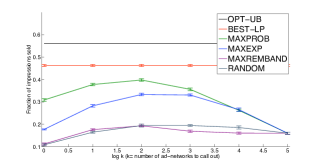
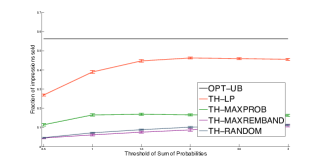
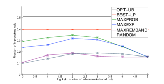
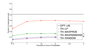
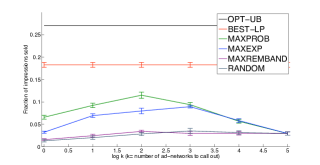
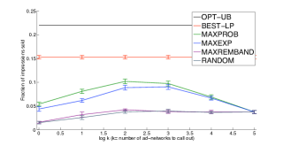
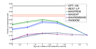
We tried our algorithms for 2000 impressions in each simulation. While this stream may seem small, we checked the standard deviation of our results when different streams drawn from the same distribution were used, and found them to be sufficiently small. With $10$ different such streams, the standard deviation was found to be about $2\%$ or less for all the algorithms. The performance (along with error bars indicating the deviation) of the various strategies are plotted in Figures 1, 2 and 3. While the performance of threshold algorithms are plotted against the threshold parameter, that of the set based algorithms are plotted against $k$ on a logarithmic scale, that is, $\log k$. BEST-LP indicates the performance of our LP-based algorithm for optimal choice of threshold, and is shown along with set based algorithms for comparison. OPT-UB indicates the upper bound on an optimal policy that is given by LP1 in the previous section. Note that the real offline optimum can be significantly smaller, but is hard to compute. The following conclusions emerge:

(Gaussian)	(Pareto)

Figure 4: Set-based algorithms for different bid distributions with erroneous bid estimations

1. The LP-based algorithm surpasses the performance of the other algorithms by a large margin, about $20\%$ more than the closest performer with optimal parameter choice. This gap grows to $85\%$ when the reserve prices are raised, and the performance of all the algorithms (and also the optimum) falls. Thus, our LP-based algorithm is even more valuable in a world where fewer items can be sold. Figure  3, show the effect of raising the minimum prices for set based algorithms.

2. The algorithms Random and MaxRemBand perform quite poorly compared to all other algorithms that use information about bid distributions. This shows that bid estimation is useful.

3. The performance of MaxExp was better than Random and MaxRemBand, but was worse than MaxProb. Thus for the distribution used in the simulation, information about expectation was useful, but less useful than the survival probability of the bids.

4. The other threshold based algorithms perform quite poorly. In the rest of the experimental evaluation, we will ignore these algorithms.

7.3 Robustness and Error estimation

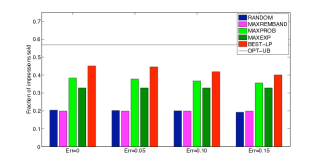
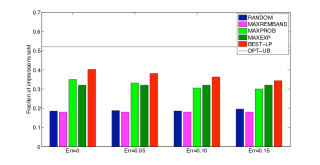
Estimating survival probabilities can be a tough problem, and can be loosely compared to the problem of estimating click-through-rates. It is thus very likely that the estimates will be inaccurate, and it is very important to understand how useful such erroneous estimates are. We add noises to the survival probabilities that are normally distributed (round to $0$ or $1$ if the resulting value is below $0$ or above $1$, respectively), and have standard deviations ranging from $0.05$ to $0.15$. We find that the algorithms using this information lose some performance, but still perform consistently better than the algorithms without any information about bid distributions. We show the plots for both distributions, in Figure 4. For comparison, we choose to represent an algorithm by its peak performance, that is, its performance for optimal choice of parameters.

Figure 5: Set based algorithms for Pareto bid distributions with burst sizes $2$, $5$ and $15$

7.4 Sensitivity analysis

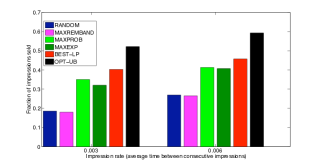
For all the plots described above, the size of the token buckets were fixed at $5$ and the arrival rate was fixed to $0.003$. We tried out bucket sizes of $2$, $5$, $15$, and $45$. As expected, the performance of each algorithm is greater when bucket size is larger; but there was no substantial differences in the conclusions we observed. In fact, the performance of the algorithms were within a standard deviation of a different bucket size (we omit showing them to avoid clutter) There was no difference in performance between bucket sizes $15$ and $45$. We superimpose the performance plots of bucket sizes $2,5,15$ and show this plot for Pareto distributions in Figure 5. We also varied impression arrival rate to note its effect on our algorithms. We found, as expected, that performance improves if arrival rate slows down, but the relative performances of the algorithms remain unchanged. Figure 6 shows this for the peak performances of the algorithms, for Pareto bid distributions.

The plots for Gaussian distributions and threshold algorithms are similar in both cases.

Figure 6: Peak performances of algorithms for different impression arrival rates for Pareto bid distributions

8 Conclusion & Future Work

We initiate a formal study of bandwidth and resource constraints faced by ad exchanges and ad networks as they move into the arena of real time bid solicitation. Our conceptual framework of learning bid distribution followed by online decision making should be useful for further study of real time bidding systems. Our online algorithms are fast and can be implemented to run in real time within this conceptual framework. The technical framework of our algorithm, with a short learning phase followed by a long online phase, can generally be applied to any problem that involves maximizing linear objectives, or objectives that can be approximated by a concave or linear objective, with linear constraints.

Appendix A The Adversarial Model

We show that no online algorithm, deterministic or randomized, can give any approximation to the offline optimum, even when the instance has only one ad network, and the bids are $0$ or $1$.

Theorem 6

For any given $0<\alpha\leq 1$, there exists no randomized algorithm which is $\alpha$-approximate, if the length of the sequence is arbitrarily large.

Proof: Maximizing the sales objective in the presence of only one ad network subsumes the online knapsack problem (the value of an item is the probability that the bid exceeds minimum price) with unit size of items, for which no algorithm can give better than $1/\Omega(\log m)$ approximation [18]. If $m$ is allowed to be large, then no algorithm giving approximation independent of $m$ can exist.      

One key feature of the adversarially constructed sequences in the theorem above is that OPT can be arbitrarily small compared to the length of the sequence. This is unlikely to happen; moreover, if it were to happen, then there would not be much benefit out of constructing the real time bidding system. Thus we make the assumption that OPT is reasonably large. But even with that assumption, we don’t fare particularly well. Following is a simple observation about sales.

Lemma A.1

For a given impression $j$, suppose ad network $i$, with survival probability $p_{ij}$ is called out with probability $x_{ij}$. Then the probability of selling the impression is $1-\prod_{i=1}^{n}(1-p_{ij}x_{ij})$. If $\sum_{i=1}^{n}p_{ij}x_{ij}=c$, then the probability of selling the impression is at most $c$ and at least $1-\frac{1}{e^{c}}$.

Proof: The probability of selling the impression is $1-\prod_{i=1}^{n}(1-p_{ij}x_{ij})$. It is upper bounded by $\sum_{i}p_{ij}x_{ij}=c$. The probability is lower bounded by $1-\prod_{i=1}^{n}(1-c/n)^{n}$ where $n$ is the number of ad-networks, and this is lower bounded by $1-\frac{1}{e^{c}}$.      

Theorem 7

Suppose it is promised that $\mbox{\sf OPT}\geq\delta m$, where $\delta>0$ is known to the algorithm. Then, no algorithm can be better than $1/\Omega(\log(1/\delta))$-approximate for the sales or total value objective. Moreover, a simple randomized algorithm is $1/O(\log(n/\delta))$-approximate for the sales objective.

Proof: The hardness instances for online knapsack problems also imply that if the value of all items are guaranteed to lie between $L$ and $U$, $L<U$, then no algorithm can give better than $1/\Omega(\log(U/L))$ approximation [18], if $m$ is allowed to be arbitrarily large. The promise $\mbox{\sf OPT}\geq\delta m$ allows us to construct any instance where values of items range from $\delta$ to $1$, thus yielding the lower bound. For the upper bound on sales, we use the following simple algorithm: Let us assume, wlog, that $\delta$ is a negative power of $2$. Choose a random cut-off $t$ from the set $H=\{\delta/2,\delta,2\delta,4\delta\ldots 1\}$. Now send each impression to any $2/t$ ad networks who has survival probability between $t$ and $2t$ and has bandwidth remaining. If there are less than $2/t$ such qualifying ad networks for an impression, then send it to all qualifying ad networks. This algorithm gives a $1/O(\log(n/\delta))$ approximation; the proof is standard.

References

- [1] Y. Azar, B. E. Birnbaum, A. R. Karlin, and C. T. Nguyen. On revenue maximization in second-price ad auctions. Proc. of ESA, pages 155–166, 2009.
- [2] M. Babaioff, N. Immorlica, D. Kempe, and R. Kleinberg. Knapsack secretary problem with applications. Proceedings of Approx, pages 16–28, 2007.
- [3] R. E. Barlow, A. W. Marshall, and F. Proschan. Properties of probability distributions with monotone hazard rate. The Annals of Mathematical Statistics, 34(2):375–389, 1963.
- [4] S. Bhattacharya, G. Goel, S. Gollapudi, and K. Munagala. Budget constrained auctions with heterogeneous items. STOC, also at http://arxiv.org/abs/0907.4166, 2010.
- [5] N. Buchbinder, K. Jain, and J. Naor. Online primal-dual algorithms for maximizing ad-auctions revenue. Proc. of ESA, pages 253–264, 2007.
- [6] G. Calinescu, C. Chekuri, M. Pál, and J. Vondrák. Maximizing a submodular set function subject to a matroid constraint (extended abstract). IPCO, pages 182–196, 2007.
- [7] D. Chakrabarty and G. Goel. On the approximability of budgeted allocations and improved lower bounds for submodular welfare maximization and gap. Proceedings of FOCS, pages 687–696, 2008.
- [8] S. Chawla, J. Hartline, D. Malec, and B. Sivan. Sequential posted pricing and multi-parameter mechanism design. STOC, also at http://arxiv.org/abs/0907.2435, 2010.
- [9] N. Devanur and T. Hayes. The adwords problem: Online keyword matching with budgeted bidders under random permutations. In Proc. 10th Annual ACM Conference on Electronic Commerge (EC), 2009.
- [10] A. Ghosh, P. McAfee, K. Papineni, and S. Vassilvitskii. Bidding for representative allocations for display advertising. In Proc. of 5th Workshop on Internet and Economics(WINE), 2009.
- [11] A. Ghosh, B. I. P. Rubinstein, S. Vassilvitskii, and M. Zinkevich. Adaptive bidding for display advertising. In WWW, pages 251–260, 2009.
- [12] S. Guha and A. McGregor. Approximate quantiles and the order of the stream. Proc. of PODS, pages 273–279, 2006.
- [13] S. Guha and K. Munagala. Adaptive uncertainty resolution in bayesian combinatorial optimization problems. ACM Transactions of Algorithms, (to appear).
- [14] J. Kleinberg, Y. Rabani, and E. Tardos. Allocating bandwidth for bursty connections. SIAM J. Of Computing, 30(1):171–217, 2001.
- [15] R. Kleinberg. A multiple-choice secretary problem with applications to online auctions. Proceedings of SODA, pages 630–631, 2005.
- [16] R. Kleinberg, A. Slivkins, and E. Upfal. Multi-armed bandits in metric spaces. In STOC, pages 681–690, 2008.
- [17] A. Kulik, H. Shachnai, and T. Tamir. Maximizing submodular set functions subject to multiple linear constraints. SODA, pages 545–554, 2009.
- [18] A. Marchetti-Spaccamela and C. Vercellis. Stochastic on-line knapsack problems. Mathematical Programming, 68:73–104, 1995.
- [19] A. Mehta, A. Saberi, U. Vazirani, and V. Vazirani. Adwords and generalized on-line matching. In FOCS, pages 264–273, 2005.
- [20] S. Muthukrishnan. Adexchange: Research issues. In Proc. of 5th Workshop on Internet and Economics(WINE), 2009.
- [21] R. B. Myerson. Optimal auction design. Math. of OR, 6(1):58–73, 1981.
- [22] M. Nolet. http://www.mikeonads.com/2009/08/30/rtb-part-i-what-is-it/.
- [23] S. Pandey and C. Olston. Handling advertisements of unknown quality in search advertising. Proceedings of NIPS, pages 1065–1072, 2006.
- [24] P. release. http://www.doubleclick.com/insight/ blog/archives/doubleclick-advertising-exchange/announcing-the-new-doubleclick-ad-exchange.html.
- [25] R. T. Rockafellar. Convex Analysis. Princeton University Press, 1970.
- [26] A. S. Tanenbaum. Computer Networks, 3rd Edition. Prentice-Hall, 1996.
- [27] E. Vee, S. Vassilvitskii, and J. Shanmugasundaram. Optimal online assignment with forecasts. In EC, 2010.