A mollified ensemble Kalman filter

Abstract

It is well recognized that discontinuous analysis increments of sequential data assimilation systems, such as ensemble Kalman filters, might lead to spurious high frequency adjustment processes in the model dynamics. Various methods have been devised to continuously spread out the analysis increments over a fixed time interval centered about analysis time. Among these techniques are nudging and incremental analysis updates (IAU). Here we propose another alternative, which may be viewed as a hybrid of nudging and IAU and which arises naturally from a recently proposed continuous formulation of the ensemble Kalman analysis step. A new slow-fast extension of the popular Lorenz-96 model is introduced to demonstrate the properties of the proposed mollified ensemble Kalman filter.

1 Introduction

Given a model in form of an ordinary differential equation and measurements at discrete instances in time, data assimilation attempts to find the best possible approximation to the true dynamics of the physical system under consideration (Evensen, 2006). Data assimilation by sequential filtering techniques achieves such an approximation by discontinuous-in-time adjustment of the model dynamics due to available measurements. While optimality of the induced continuous-discrete filtering process can be shown for linear systems, discontinuities can lead to unphysical readjustment processes under the model dynamics for nonlinear systems and under imperfect knowledge of the error probability distributions. See, e.g., Houtekamer and Mitchell (2005); Kepert (2009) in the context of operational models as well as Neef et al. (2006); Oke et al. (2007) for a study of this phenomena under simple model problems. These observations have led to the consideration of data assimilation systems that seek to incorporate data in a more “continuous” manner. In this paper we focus on a novel continuous data assimilation procedure based on ensemble Kalman filters. Contrary to widely used incremental analysis updates (IAU) of Bloom et al. (1996), which first do a complete analysis step to then distribute the increments evenly over a given time window, our approach performs the analysis step itself over a fixed window. Our novel filter technique is based on the continuous formulation of the Kalman analysis step in terms of ensemble members (Bergemann and Reich, 2010) and mollification of the Dirac delta function by smooth approximations (Friedrichs, 1944). The proposed mollified ensemble Kalman (MEnK) filter is described in Section 2. The MEnK filter may be viewed as a “sophisticated” form of nudging (Hoke and Anthes, 1976; Macpherson, 1991) with the nudging coefficients being obtained from a Kalman analysis perspective instead of heuristic tuning. However, for certain multi-scale systems, nudging with prescribed nudging coefficients might still be advantageous (Ballabrera-Poy et al., 2009). We also point to the closely related work by Lei and Stauffer (2009), which proposes a nudging-type implementation of the ensemble Kalman filter with perturbed observations (Burgers et al., 1998).

To demonstrate the properties of the new MEnK filter, we propose a slow-fast extension of the popular Lorenz-96 model (Lorenz, 1996) in Section 4. Contrary to other multi-scale extensions of the Lorenz-96 model, the fast dynamics is entirely conservative in our model and encodes a dynamic balance relation similar to geostrophic balance in primitive equation models. Our model is designed to show the generation of unbalanced fast oscillations through standard sequential ensemble Kalman filter implementations under imperfect knowledge of the error probability distributions. Imperfect knowledge of the error probability distribution can arise for various reasons. In this paper, we address in particular the aspect of small ensemble size and covariance localization (Houtekamer and Mitchell, 2001; Hamill et al., 2001). It is also demonstrated that both IAU as well as the newly proposed MEnK filter maintain balance under assimilation with small ensembles and covariance localization. However, IAU develops an instability in our model system over longer assimilation cycles, which requires a relatively large amount of artificial damping in the fast dynamics. We also note that the MEnK filter is cheaper to implement than IAU since no complete assimilation cycle and repeated model integration need to be performed. It appears that the MEnK filter could provide a useful alternative to the widely employed combination of data assimilation and subsequent ensemble re-initialization. See, for example, Houtekamer and Mitchell (2005).

2 Mollified ensemble Kalman filter

We consider models given in form of ordinary differential equations

$$\dot{\bf x}=f({\bf x},t)$$ (1)

with state variable ${\bf x}\in\mathbb{R}^{n}$. Initial conditions at time $t_{0}$ are not precisely known and we assume instead that

$${\bf x}(t_{0})\sim{\rm N}({\bf x}_{0},{\bf B}),$$ (2)

where ${\rm N}({\bf x}_{0},{\bf B})$ denotes an $n$-dimensional Gaussian distribution with mean ${\bf x}_{0}\in\mathbb{R}^{n}$ and covariance matrix ${\bf B}\in\mathbb{R}^{n\times n}$. We also assume that we obtain measurements ${\bf y}(t_{j})\in\mathbb{R}^{p}$ at discrete times $t_{j}\geq t_{0}$, $j=0,1,\ldots,M$, subject to measurement errors, which are also Gaussian distributed with zero mean and covariance matrix ${\bf R}\in\mathbb{R}^{p\times p}$, i.e.

$${\bf y}(t_{j})-{\bf H}{\bf x}(t_{j})\sim{\rm N}({\bf 0},{\bf R}).$$ (3)

Here ${\bf H}\in\mathbb{R}^{p\times n}$ is the (linear) measurement operator.

Ensemble Kalman filters (Evensen, 2006) rely on the simultaneous propagation of $m$ independent solutions ${\bf x}_{i}(t)$, $i=1,\ldots,m$, of (1), which we collect in a matrix ${\bf X}(t)\in\mathbb{R}^{n\times m}$. We can extract an empirical mean

$$\overline{\bf x}(t)=\frac{1}{m}\sum_{i=1}^{m}{\bf x}_{i}(t)$$ (4)

and an empirical covariance matrix

$${\bf P}(t)=\frac{1}{m-1}\sum_{i=1}^{m}\left({\bf x}_{i}(t)-\overline{\bf x}(t)\right)\left({\bf x}_{i}(t)-\overline{\bf x}(t)\right)^{T}$$ (5)

from the ensemble. In typical applications from meteorology, the ensemble size $m$ is much smaller than the dimension $n$ of the model phase space. We now state a complete ensemble Kalman filter formulation for sequences of observations at time instances $t_{j}$, $j=1,\ldots,M$, and intermediate propagation of the ensemble under the dynamics (1). Specifically, the continuous formulation of the ensemble Kalman filter step by Bergemann and Reich (2010) allows for the following concise formulation in terms of a single differential equation

$$\dot{\bf x}_{i}=f({\bf x}_{i},t)-\sum_{j=1}^{M}\delta(t-t_{j})\,{\bf P}\nabla_{{\bf x}_{i}}{\cal V}_{j}({\bf X})$$ (6)

in each ensemble member, where $\delta(\cdot)$ denotes the standard Dirac delta function, ${\cal V}_{j}$ is the potential

$${\cal V}_{j}({\bf X})=\frac{m}{2}\left\{S_{j}(\overline{\bf x})+\frac{1}{m}\sum_{i=1}^{m}S_{j}({\bf x}_{i})\right\}$$ (7)

with observational cost function

$$S_{j}({\bf x})=\frac{1}{2}\left({\bf H}{\bf x}-{\bf y}(t_{j})\right)^{T}{\bf R}^{-1}\left({\bf H}{\bf x}-{\bf y}(t_{j})\right).$$ (8)

One may view (6) as the original ODE (1) driven by a sequence of impulse like contributions due to observations. See the Appendix for a derivation of (6).

It should be noted that (6) is equivalent to a standard Kalman filter (and hence optimal) for linear models and the number of ensemble members $m$ larger than the dimension of phase space $n$. This property does no longer hold under nonlinear model dynamics and it makes sense to “mollify” the discontinuous analysis adjustments as, for example, achieved by the popular IAU technique (Bloom et al., 1996). In the context of (6), a most natural mollification is achieved by replacing (6) with

$$\dot{\bf x}_{i}=f({\bf x}_{i},t)-\sum_{j=1}^{M}\delta_{\epsilon}(t-t_{j})\,{\bf P}\nabla_{{\bf x}_{i}}{\cal V}_{j}({\bf X}),$$ (9)

where

$$\delta_{\epsilon}(s)=\frac{1}{\epsilon}\psi(s/\epsilon),$$

$\psi(s)$ is the standard hat function

$$\psi(s)=\left\{\begin{array}[]{ll}1-|s|&\mbox{for}\,\,|s|\leq 1,\\ 0&\mbox{else}\end{array}\right.$$ (10)

and $\epsilon>0$ is an appropriate parameter. The hat function (10) could, of course, be replaced by another B-spline. We note that the term mollification was introduced by Friedrichs (1944) to denote families of compactly supported smooth functions $\delta_{\epsilon}$ which approach the Dirac delta function $\delta$ in the limit $\epsilon\to 0$. Mollification via convolution turns non-standard functions (distributions) into smooth functions. Here we relax the smoothness assumption and allow for any non-negative, compactly supported family of functions that can be used to approximate the Dirac delta function. A related mollification approach to numerical time-stepping methods has been proposed in the context of multi-rate splitting methods for highly oscillatory ordinary differential equations in García-Archilla et al. (1998); Izaguirre et al. (1999).

Formulations (6) and (9) are based on square-root filter formulations of the ensemble Kalman filter (Tippett et al., 2003). Ensemble inflation (Anderson and Anderson, 1999) is a popular techniques to stabilize the performance of such filters. We note that ensemble inflation can be interpreted as adding a $\theta\left({\bf x}_{i}-\overline{\bf x}\right)$ term to the right hand side of (9) for an appropriate parameter value $\theta>0$. We note that a related “destabilizing” term appears in $H_{\infty}$ continuous filter formulations for linear systems. See, for example, Simon (2006) for details. The link to $H_{\infty}$ filtering suggests alternative forms of ensemble inflation and a systemtic approach to make ensemble Kalman filters more robust. Details will be explored in a forthcoming publication.

Localization (Houtekamer and Mitchell, 2001; Hamill et al., 2001) is another popular technique to enhance the performance of ensemble Kalman filters. Localization can easily be implemented into the mollified formulation (9) and leads to a modified covariance matrix $\widetilde{\bf P}={\bf C}\circ{\bf P}$ in (9). Here ${\bf C}$ is an appropriate localization matrix and ${\bf C}\circ{\bf P}$ denotes the Schur product of ${\bf C}$ and ${\bf P}$. See Bergemann and Reich (2010) for details.

We finally note that both (6) and (9) can be modified to become consistent with an ensemble Kalman filter with perturbed observations (Burgers et al., 1998). This requires to adjust the potentials ${\cal V}_{j}$ and to add a stochastic forcing term.

3 Algorithmic summary

Formulation (9) can be solved numerically by any standard ODE solver. Similar to nudging, there is no longer a strict separation between ensemble propagation and filtering. However, based on (9), “nudging” is performed consistently with Kalman filtering in the limit $\epsilon\to 0$. An optimal choice of $\epsilon$ will depend on the specific applications.

Using, for example, the implicit midpoint method as the time-stepping method for the dynamic part of (9) and denoting numerical approximations at $t_{k}=k\Delta t$ by ${\bf x}_{i}^{k}$, we obtain the following algorithm:

$${\bf x}_{i}^{k+1}={\bf x}_{i}^{k}+\Delta t\left\{f({\bf x}_{i}^{k+1/2},t_{k+1/2})-\sum_{j=1}^{M}\alpha_{j}^{k}{\bf P}^{k}\nabla_{{\bf x}_{i}}{\cal V}_{j}({\bf X}^{k})\right\},$$ (11)

for $i=1,\ldots,m$. Here ${\bf X}^{k}$ is the collection of ensemble approximations at $t_{k}$, ${\bf P}^{k}$ is the resulting covariance matrix, ${\bf x}_{i}^{k+1/2}=({\bf x}_{i}^{k+1}+{\bf x}_{i}^{k})/2$ is the midpoint approximation, and the weights $\alpha_{j}^{k}\geq 0$ are defined by

$$\alpha_{j}^{k}=\frac{c}{\epsilon}\psi\left(\frac{t_{k}-j\Delta t_{\rm obs}}{\epsilon}\right)$$ (12)

with the hat function (10) and normalization constant $c>0$ chosen such that

$$\Delta t\sum_{k}\alpha_{j}^{k}=1.$$ (13)

Note that the summation in (11) needs to be performed only over those (measurement) indices $j$ with $\alpha_{j}^{k}\not=0$.

For the numerical experiments conducted in this paper, we set $\epsilon=\Delta t_{\rm obs}/2$ and assume that $\Delta t_{\rm obs}$ is a multiple of the time-step size $\Delta t$. Under this setting only a single measurment ${\bf y}(t_{j})$ is assimilated at any given time-step $t_{k}$. Another interesting choice is $\epsilon=\Delta t_{\rm obs}$ which implies that $\sum_{j}\alpha_{j}^{k}$ is independent of the time-step index $k$. In this case, two measurements are simultaneously assimilated (with different weights) at any given time-step $t_{k}$.

The main additional cost of (11) over standard implementations of ensemble Kalman filters is the computation of the covariance matrix ${\bf P}$ in each time-step. However, this cost is relatively minor compared to the cost involved in propagating the ensemble under the model equations (1) in the context of meteorological applications. We note that, contrary to IAU and the recent work by Lei and Stauffer (2009), no additional model propagation steps are required.

4 A slow-fast Lorenz-96 model

We start from the standard Lorenz-96 model (Lorenz, 1996; Lorenz and Emanuel, 1998)

$$\dot{x}_{l}=(x_{l+1}-x_{l-2})x_{l-1}-x_{l}+8$$ (14)

for $l=1,\ldots,40$ with periodic boundary conditions, i.e., $x_{-1}=x_{39}$, $x_{0}=x_{40}$, and $x_{41}=x_{1}$. We note that the energy

$$E_{\rm Lorenz}=\frac{1}{2}\sum_{l=1}^{40}x_{l}^{2}$$ (15)

is preserved under the “advective” contribution

$$\dot{x}_{l}=(x_{l+1}-x_{l-2})x_{l-1}=x_{l-1}x_{l+1}-x_{l-2}x_{l-1}$$ (16)

to the Lorenz-96 model.

We now derive a slow-fast extension of (14). To do so we introduce an additional variable $h$, which satisfies a discrete wave equation, i.e.,

$$\varepsilon^{2}\ddot{h}_{l}=-h_{l}+\alpha^{2}\left[h_{l+1}-2h_{l}+h_{l-1}\right],$$ (17)

$l=1,\ldots,40$, where $\varepsilon>0$ is a small parameter implying that the time evolution in $h$ is fast compared to that of $x$ in the Lorenz model (14) and $\alpha>0$ is a parameter determining the wave dispersion over the computational grid. We assume again periodic boundary conditions and find that (17) conserves the energy

$$E_{\rm wave}=\frac{\varepsilon^{2}}{2}\sum_{l=1}^{40}\dot{h}_{l}^{2}+\frac{1}{2}\sum_{l=1}^{40}\left[h_{l}^{2}+\alpha^{2}\left(h_{l+1}-h_{l}\right)^{2}\right].$$ (18)

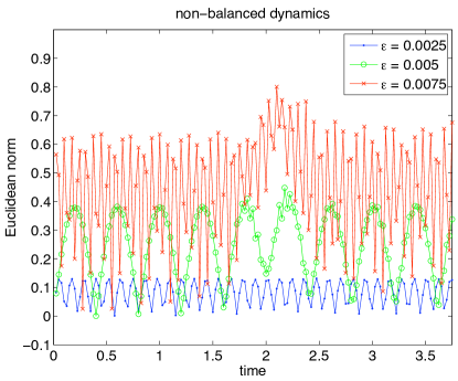
Figure 1: Norm of (27) over all grid points for several values of $\varepsilon$ as a function of integration time. It can be concluded that balance is maintained to high accuracy for sufficiently small values of $\varepsilon$ except for perturbations induced at initial time. The amplitude of the oscillations could be reduced further by more sophisticated initialization techniques (higher order balance conditions).

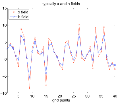
Figure 2: Typical balanced $\{x_{l}\}$ and $\{h_{l}\}$ fields for the slow-fast Lorenz model. It can be seen that the balanced $\{h_{l}\}$ is more regular than the $\{x_{l}\}$ field due to the balance relation (26).

The two models (14) and (17) are now coupled together by introducing an exchange energy term

$$E_{\rm coupling}=-\delta\sum_{l=1}^{40}h_{l}x_{l},$$ (19)

where $\delta>0$ characterizes the coupling strength. The equations of motion for the combined system are then defined as

$$\dot{x}_{l} = (1-\delta)\left(x_{l+1}-x_{l-2}\right)x_{l-1}+\delta\left(x_{l-1}h_{l+1}-x_{l-2}h_{l-1}\right)-x_{l}+8,$$ (20)

$$\varepsilon^{2}\ddot{h}_{l} = -h_{l}+\alpha^{2}\left[h_{l+1}-2h_{l}+h_{l-1}\right]+x_{l},$$ (21)

where we have scaled the advective contribution in (14) by a factor of $1-\delta$ to counterbalance the additional contribution from the coupling term. We note that the pure wave-advection system

$$\dot{x}_{l} = (1-\delta)\left(x_{l+1}-x_{l-2}\right)x_{l-1}+\delta\left(x_{l-1}h_{l+1}-x_{l-2}h_{l-1}\right),$$ (22)

$$\varepsilon^{2}\ddot{h}_{l} = -h_{l}+\alpha^{2}\left[h_{l+1}-2h_{l}+h_{l-1}\right]+x_{l}$$ (23)

conserves the total energy

$$H = (\delta-1)E_{\rm Lorenz}+\delta E_{\rm wave}+E_{\rm coupling}$$ (24)

$$= \frac{\delta}{2}\sum_{l=1}^{40}\left\{\frac{\delta-1}{\delta}x_{l}^{2}+\varepsilon^{2}\dot{h}_{l}^{2}+h_{l}^{2}+\alpha^{2}\left(h_{l+1}-h_{l}\right)^{2}-2x_{l}h_{l}\right\}$$ (25)

independent of the choice of $\delta\in[0,1]$. We also wish to point to the balance relation

$$x_{l}=h_{l}-\alpha^{2}\left[h_{l+1}-2h_{l}+h_{l-1}\right]$$ (26)

in the wave part (21). More specifically, if (26) is satisfied at initial time, the variables $\{h_{l}\}$ and $\{x_{l}\}$ will remain in approximate balance over a fixed time interval with the deviation from exact balance proportional to $\varepsilon$ (Wirosoetisno and Shepherd, 2000; Wirosoetisno, 2004; Cotter and Reich, 2006). We demonstrate conservation of balance for decreasing values of $\varepsilon$ in Fig. 1, where we display the Euclidean norm of

$${\Delta}_{l}=x_{l}-h_{l}+\alpha^{2}\left[h_{l+1}-2h_{l}+h_{l-1}\right],$$ (27)

$l=1,\ldots,40$, as a function of time. Hence, we may view (26) as defining an approximative slow manifold on which the dynamics of (20)-(21) essentially reduces to the dynamics of the standard Lorenz-96 model for sufficiently small $\varepsilon$. We use $\varepsilon=0.0025$ for our numerical experiments. On the other hand, any imbalance introduced through a data assimilation system will remain in the system since there is no damping term in (21). This is in contrast to other slow-fast extensions of the Lorenz-96 model, such as Lorenz (1996), which also introduce damping and forcing into the fast degrees of freedom. We will find in Section 5 that some ensemble Kalman filter implementations require the addition of an “artificial” damping term into (21) and we will use

$$\varepsilon^{2}\ddot{h}_{l}=-h_{l}+\alpha^{2}\left[h_{l+1}-2h_{l}+h_{l-1}\right]+x_{l}-\gamma\varepsilon^{2}\dot{h}_{l}$$ (28)

for those filters with an appropriately chosen parameter $\gamma>0$.

We mention that (20)-(21) may be viewed as an one-dimensional “wave-advection” extension of the Lorenz-96 model under a quasi-geostrophic scaling regime with $\varepsilon$ being proportional to the Rossby number and ${\rm Bu}=\alpha^{2}$ being the Burger number (Salmon, 1999). In a quasi-geostrophic regime, the Burger number should be of order one and we set $\alpha=1/2$ in our experiments. Since a typical time-scale of the Lorenz-96 model is about $0.025$ units, we derive at an equivalent Rossby number of $\mbox{Ro}\approx 0.1$ for $\varepsilon=0.0025$. Typical $\{h_{l}\}$ and $\{x_{l}\}$ fields are displayed in Fig. 2. It should, of course, be kept in mind that the Lorenz-96 model is not the discretization of a realistic fluid model.

The dynamics of our extended model depends on the coupling strength $\delta\in[0,1]$. Since the $\{h_{l}\}$ field is more regular than the $\{x_{l}\}$ field, stronger coupling leads to a more regular dynamics in terms of spatial correlation. We compute the grid-value mean $\overline{x}=\langle x_{l}\rangle$ and its variance $\sigma=\langle(x_{l}-\bar{x})^{2}\rangle^{1/2}$ along a long reference trajectory for $\delta=0.1$ ($\bar{x}=2.32$, $\sigma=3.68$), $\delta=0.5$ ($\bar{x}=1.80$, $\sigma=3.67$), and $\delta=1.0$ ($\bar{x}=1.48$, $\sigma=3.69$), respectively. The variance is nearly identical for all three parameter values while the mean decreases for larger values of $\delta$, which implies that the dynamics becomes less “non-linear” for larger values of $\delta$.

5 Numerical experiments

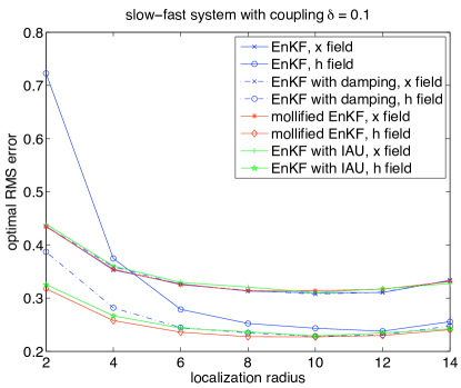
Figure 3: Best RMS error for slow-fast Lorenz-96 model with coupling strength $\delta=0.1$ using ensembles of size $m=10$ and $k=20$ observations of $\{x_{j}\}$ taken in intervals of $\Delta t_{\rm obs}=0.05$ over a total of 4000 assimilation cycles. We compare a standard ensemble Kalman filter (EnKF) implementation to the MEnK filter and a EnKF with IAU. We also implement a standard EnKF for the damped wave equation (28) with damping factor $\gamma=0.1$.

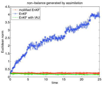
Figure 4: Unbalanced dynamics generated through the data assimilation steps in a standard ensemble Kalman filter (EnKF) implementation as compared to the relatively low and nearly constant unbalanced wave activities under the MEnK filter and the IAU EnKF implementation over 500 assimilation steps and for coupling constant $\delta=0.1$ and localization radius $r_{0}=2$.

We run the system for a coupling strengths of $\delta=0.1$ and $\delta=0.5$, respectively, using either a (standard) ensemble Kalman filter implementation based on (6) or an implementation of the mollified formulation (9). We also recall that the mollified formulation (9) uses the mollifier (10) with $\epsilon=\Delta_{\rm obs}/2$.

We observe $\{x_{l}\}$ at every second grid point in time-intervals of $\Delta t_{\rm obs}=0.05$ with measurement error variance ${\bf R}={\bf I}_{20}$. The time-step for the numerical time-stepping method (a second-order in time, time-symmetric splitting method (Leimkuhler and Reich, 2005)) is $\Delta t=\Delta t_{\rm obs}/20=0.0025$.

All filter implementations use localization (Houtekamer and Mitchell, 2001; Hamill et al., 2001) and ensemble inflation (Anderson and Anderson, 1999). Localization is performed by multiplying each element of the covariance matrix ${\bf P}$ by a distance dependent factor $\rho_{i,i^{\prime}}$. This factor is defined by the compactly supported localization function (4.10) from Gaspari and Cohn (1999), distance $r_{l,l^{\prime}}=\min\{|l-l^{\prime}|,40-|l-l^{\prime}|\}$, where $l$ and $l^{\prime}$ denote the indices of the associated observation/grid points $x_{l}$ and $x_{l^{\prime}}$, respectively, and a fixed localization radius $r_{0}$. See Bergemann and Reich (2010) for more implementation details. Inflation is applied after each time-step to the $\{x_{l}\}$ components of the ensemble members.

The initial ensemble is generated by adding small random perturbations to a reference $\{x_{l}\}$ field. The associated $\{h_{l}\}$ ensemble fields are computed from the balance relation (26). After a spin-up period of 200 assimilation cycles, we do a total of 4000 assimilation cycles in each simulation run and compute the RMS error between the analyzed predictions and the true reference solution from which the measurements were generated. RMS errors are computed over a wide range of inflation factors and only the optimal result for a given localization radius is reported.

We first compare the performance of a standard ensemble Kalman filter implementation with the proposed MEnK filter for a coupling strength $\delta=0.1$. It can be seen from Fig. 3 that the RMS error in the $\{h_{l}\}$ fields is much larger for the standard ensemble Kalman filter than for the mollified scheme. The difference is most pronounced for small localization radii. Indeed, it is found that the standard filter generates significant amounts of unbalanced waves. See Fig. 4, where we display the Euclidean norm of (27) over all ensemble members for the first 500 assimilation steps and localization radius $r_{0}=2$. Note that ${\Delta}_{l}=0$ at $t=0$ and that no damping is applied to the wave part (21). We also implement a standard ensemble Kalman filter for the damped wave equation (28) with $\gamma=0.1$ which leads to a significant reduction (but not complete elimination) in the RMS errors for the $\{h_{l}\}$ fields. Qualitatively the same results are obtained for the stronger coupling $\delta=0.5$, see Fig. 5.

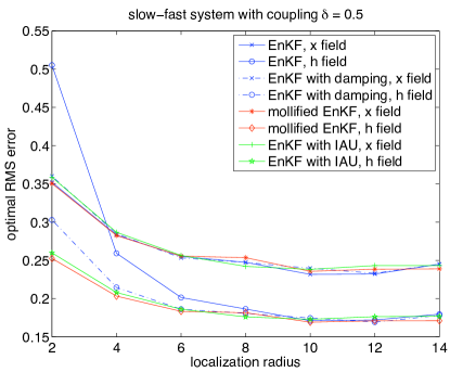
Figure 5: Same as Fig. 3 except that the coupling strength is set to $\delta=0.5$.

For comparison we implement an IAU along the lines of Bloom et al. (1996); Polavarapu et al. (2004) with the analysis increments provided by a standard ensemble Kalman filter. Instead of a constant forcing, we use the hat function (10) for computing the weights $g(t)$ in Bloom et al. (1996) to be consistent with the implementation of the MEnK filter. While it is found that the resulting IAU ensemble Kalman filter conserves balance well initially (see Fig. 4), the IAU filter eventually becomes highly inaccurate and/or unstable. We believe that this failure of IAU over longer analysis cycles (here 4000) is due to an instability of the algorithm in the fast wave part (21). The instability could be caused by the non-symmetric-in-time nature of the IAU process, i.e., by the fact that one first computes a forecast, then finds the analysis increments based on the forecast and available observations, and finally repeats the forecast with assimilation increments included. It should also be kept in mind that the IAU of Bloom et al. (1996)) is based on a standard 3D Var analysis for given background covariance matrix, which is significantly different from an IAU ensemble Kalman filter implementation. A stable implementation of an IAU is achieved by replacing (21) by the damped version (28) with $\gamma=1.0$. Smaller values of $\gamma$ lead to filter divergence. With damping included, the IAU filter behaves almost identical to the MEnK filter and the standard ensemble Kalman filter with damping in the wave part (28), see Figs. 3 and 5.

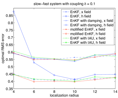
Figure 6: Same as Fig. 3 except that observations of $\{(x_{j}+h_{j})/2\}$ are taken in intervals of $\Delta t_{\rm obs}=0.05$ with measurement error variance ${\bf R}={\bf I}_{20}$ over a total of 4000 assimilation cycles.

We also tested the dependence on the type of measurements and found that observation of the mixed $\{(h_{l}+x_{l})/2\}$ field instead of $\{x_{l}\}$ leads to results which are in qualitative agreement with those displayed in Fig. 3 for all three methods, see Fig. 6.

In summary, we find that localization interferes with dynamic balance relations in standard ensemble Kalman filter implementations. This result has been well established by a number of previous studies on models of varying complexity. Here we have demonstrated for a relatively simply model system that strong localization can be used without the need of additional damping and/or re-initialization provided the assimilation increments are distributed evenly over a time-window instead of being assimilated instantaneously. It appears that the proposed MEnK filter works particularly reliably. It should be kept in mind that the MEnK filter leads to additional costs per model integration step. But these costs should be relatively small compared to those of the model dynamics itself.

6 Conclusion

In this paper, we have addressed a shortcoming of sequential data assimilation systems which arises from the discontinuous nature of the assimilation increments and the imperfect statistics under ensemble based filtering techniques. In line with the previously considered IAU and nudging techniques, we have proposed spreading the analysis through a mollified Dirac delta function. Mollification has been used before to avoid numerical instabilities in multi-rate time-stepping methods for the integration of highly oscillatory differential equations (see, for example, García-Archilla et al. (1998); Izaguirre et al. (1999)). We have demonstrated for a simple slow-fast extension of the Lorenz-96 model that the proposed MEnK filter indeed eliminates high-frequency responses in the dynamic model. The MEnK filter can be viewed as a nudging technique with the nudging coefficients determined consistently from ensemble predictions. We note in this context that a combined ensemble Kalman filter and nudging technique was found beneficial by Ballabrera-Poy et al. (2009) for the original slow-fast Lorenz-96 model (Lorenz, 1996). The MEnK filter (perhaps also combined with the filtering-nudging approach of Ballabrera-Poy et al. (2009)) may provide an alternative to currently used combinations of ensemble Kalman filters and subsequent re-initialization. For the current model study it is found that artificial damping of the unbalanced high-frequency waves stabilizes the performance of a standard ensemble Kalman filter and leads to results similar to those observed for the MEnK filter. We also found, in line with previous studies of Houtekamer and Mitchell (2005); Oke et al. (2007); Kepert (2009), that stronger localization leads to a more pronounced generation of unbalanced waves under a standard ensemble Kalman filter.

Speaking on a more abstract level, the MEnK filter also provides a step towards a more integrated view on dynamics and data assimilation. The MEnK filter is closer to the basic idea of filtering in that regard than the current practice of batched assimilation in intervals of 6 to 9 hours, which is more in line with four dimensional variational data assimilation (which is a smoothing technique). The close relation between our mollified ensemble Kalman filter, continuous time Kalman filtering and nudging should also allow for an alternative approach to the assimilation of non-synoptic measurements (Evensen, 2006).

An IAU ensemble Kalman filter has also been implemented. It is observed that the filter eventually becomes unstable and/or inaccurate unless a damping factor of $\gamma=1.0$ is applied to the fast wave part of the modified Lorenz-96 model. We did not attempt to optimize the performance of the IAU assimilation approach. It is feasible that optimally chosen weights (see Polavarapu et al. (2004) for a detailed discussion) could lead to a stable and accurate performance similar to the proposed MEnK filter. It should be noted that the MEnK filter requires less model integration steps than the IAU ensemble Kalman filter. The same statement applies to the recent work of Lei and Stauffer (2009). Indeed, the work of Lei and Stauffer (2009) is of particular interest since it demonstrates the benefit of distributed assimilation in the context of the more realistic shallow-water equations. We would also like to emphasize that IAU ensemble Kalman filtering, the hybrid approach of Lei and Stauffer (2009) and our MEnKF filter have in common that they point towards a more “continuous” assimilation of data. Such techniques might in the future complement the current operational practice of batched assimilation in intervals of, for example, 6 hours at the Canadian Meteorological Centre Houtekamer and Mitchell (2005).

We finally mention that an alternative approach to reducing the generation of unbalanced dynamics is to make covariance localization respect balance. This is the approach advocated, for example, by Kepert (2009).

Acknowledgment. We would like to thank Eugenia Kalnay for pointing us to the work on incremental analysis updates, Jeff Anderson for discussions on various aspects of ensemble Kalman filter formulations, and Bob Skeel for clarifying comments on mollification.

Appendix

We have stated in Bergemann and Reich [2010] without explicit proof that an ensemble Kalman filter analysis step at observation time $t_{j}$ is equivalent to

$${\bf x}_{i}(t_{j}^{+})={\bf x}_{i}(t_{j}^{-})-\int_{0}^{1}{\bf P}\nabla_{{\bf x}_{i}}{\cal V}_{j}({\bf X})\,{\rm d}s,$$ (29)

where ${\bf x}_{i}(t_{j}^{-})$ denotes the forecast values and ${\bf x}_{i}(t_{j}^{+})$ is the analyzed state of the $i$th ensemble member. The reader was instead referred to Simon [2006].

Before we demonstrate how (29) gives rise to (6), we provide a derivation of (29) for the simplified situation of $n=1$, $k=1$, i.e. the covariance matrices ${\bf P}$ and ${\bf R}$ are scalar quantities and the observation operator ${\bf H}$ is equal to one. Under these assumptions the standard Kalman analysis step gives rise to

$$P_{a}=\frac{P_{f}R}{P_{f}+R}$$ (30)

and

$$\overline{x}_{a}=\frac{\overline{x}_{f}R+yP_{f}}{P_{f}+R}$$ (31)

for a given observation value $y$.

We now demonstrate that this update is equivalent to twice the application of a Kalman analysis step with $R$ replaced by $2R$. Specifically, we obtain

$$P_{a}^{\prime}=\frac{2P_{m}R}{P_{m}+2R},\qquad P_{m}=\frac{2P_{f}R}{P_{f}+2R}$$ (32)

for the resulting covariance matrix $P_{a}^{\prime}$ with intermediate value $P_{m}$. The analyzed mean $\overline{x}_{a}^{\prime}$ is provided by

$$\overline{x}_{a}^{\prime}=\frac{2\overline{x}_{m}R+yP_{m}}{P_{m}+2R},\qquad\overline{x}_{m}=\frac{2\overline{x}_{f}R+yP_{f}}{P_{f}+2R}.$$ (33)

We need to demonstrate that $P_{a}=P_{a}^{\prime}$ and $\overline{x}_{a}=\overline{x}_{a}^{\prime}$. We start with the covariance matrix and obtain

$$P_{a}^{\prime}=\frac{\frac{4P_{f}R}{P_{f}+2R}R}{\frac{2P_{f}R}{P_{f}+2R}+2R}=\frac{4P_{f}R^{2}}{4P_{f}R+4R^{2}}=\frac{P_{f}R}{P_{f}+R}=P_{a}.$$ (34)

A similar calculation for $\overline{x}_{a}^{\prime}$ yields

$$\overline{x}_{a}^{\prime}=\frac{2\frac{2\overline{x}_{f}R+yP_{f}}{P_{f}+2R}R+y\frac{2P_{f}R}{P_{f}+2R}}{2R+\frac{2P_{f}R}{P_{f}+2R}}=\frac{4\overline{x}_{f}R^{2}+4yP_{f}R}{4R^{2}+4RP_{f}}=\frac{\overline{x}_{f}R+yP_{f}}{P_{f}+R}=\overline{x}_{a}.$$ (35)

Hence, by induction, we can replace the standard Kalman analysis step by $K>2$ iterative applications of a Kalman analysis with $R$ replaced by $KR$. We set $P_{0}=P_{f}$, $\overline{x}_{0}=\overline{x}_{f}$ and perform

$$P_{k+1}=\frac{KP_{k}R}{P_{k}+KR},\qquad\overline{x}_{k+1}=\frac{K\overline{x}_{k}R+yP_{k}}{P_{k}+KR}$$ (36)

for $k=0,\ldots,K-1$. We finally set $P_{a}=P_{K}$ and $\overline{x}_{a}=\overline{x}_{K}$. Next we introduce a step-size $\Delta s=1/K$ and assume $K\gg 1$. Then

$$\overline{x}_{k+1}=\frac{\overline{x}_{k}R+\Delta syP_{k}}{R+\Delta sP_{k}}=\overline{x}_{k}-\Delta sP_{k}R^{-1}\left(\overline{x}_{k}-y\right)+{\cal O}(\Delta s^{2})$$ (37)

as well as

$$P_{k+1}=\frac{P_{k}R}{R+\Delta sP_{k}}=P_{k}-\Delta sP_{k}R^{-1}P_{k}+{\cal O}(\Delta s^{2}).$$ (38)

Taking the limit $\Delta s\to 0$, we obtain the two differential equations

$$\frac{{\rm d}P}{{\rm d}s}=-PR^{-1}P,\qquad\frac{{\rm d}\overline{x}}{{\rm d}s}=-PR^{-1}\left(\overline{x}-y\right)$$ (39)

for the covariance and mean, respectively. The equation for $P$ can be rewritten in terms of its square root $Y$ (i.e. $P=Y^{2})$ as

$$\frac{{\rm d}Y}{{\rm d}s}=-\frac{1}{2}PR^{-1}Y.$$ (40)

We now consider an ensemble consisting of two members $x_{1}$ and $x_{2}$. Then $\overline{x}=(x_{1}+x_{2})/2$ and

$$P=\frac{1}{2}(x_{1}-x_{2})^{2},\qquad Y=\frac{1}{\sqrt{2}}(x_{1}-x_{2}).$$ (41)

Hence

$$\frac{\rm d}{{\rm d}s}(x_{1}+x_{2})=-PR^{-1}(x_{1}+x_{2}-2y),\qquad\frac{\rm d}{{\rm d}s}(x_{1}-x_{2})=-\frac{1}{2}PR^{-1}(x_{1}-x_{2}),$$ (42)

which gives rise to

$$\frac{{\rm d}x_{i}}{{\rm d}s}=-\frac{1}{2}PR^{-1}\left(x_{i}+\overline{x}-2y\right)$$ (43)

for $i=1,2$. Upon integrating these differential equations from $s=0$ with initial conditions $x_{i}(0)=x_{i}(t_{j}^{-})$, $i=1,2$, to $s=1$ and setting $x_{i}(t_{j}^{+})=x_{i}(1)$ we have derived a particular instance of the general continuous Kalman formulation (29).

The general, non-scalar case can be derived from a multiple application of Bayes’ theorem as follows. We denote the Gaussian prior probability distribution function by $\pi_{f}({\bf x})$ and the analyzed Gaussian probability density function by $\pi_{a}({\bf x})$. Then

$$\pi_{a}({\bf x})\propto\pi_{f}({\bf x})\times\exp(-S_{j}({\bf x}))$$ (44)

with $S_{j}({\bf x})$ defined by (8). Bayes’ formula (44) can be reformulated to

$$\pi_{a}({\bf x})\propto\pi_{f}({\bf x})\times\prod_{k=1}^{K}\exp\left(-\frac{1}{K}S_{j}({\bf x}\right),$$ (45)

which gives rise to incremental updates

$$\pi_{k+1}({\bf x})\propto\pi_{k}({\bf x})\times\exp\left(-\frac{1}{K}S_{j}({\bf x}\right)$$ (46)

for $k=0,\ldots,K-1$ with $\pi_{0}=\pi_{f}$. The incremental update in the probability density functions $\pi_{k}$ gives rise to a corresponding incremental Kalman update step, which leads to the desired continuous formulations in the limit $K\to\infty$.

Having shown that an ensemble Kalman filter analysis step is equivalent to (29), we next demonstrate that (6) is the appropriate mathematical formulation for the complete data assimilation scheme. To do so we replace the Dirac delta function $\delta(t-t_{j})$ in (6) by a function that takes the constant value $1/\epsilon$ on the interval $[t_{j}-\epsilon/2,t_{j}+\epsilon/2]$ and zero elsewhere. This function approaches the Dirac delta function as $\epsilon\to 0$. Then we obtain from (6)

$${\bf x}_{i}(t_{j}-\epsilon/2+\delta)={\bf x}_{i}(t_{j}-\epsilon/2)+\int_{0}^{\delta}\left[f({\bf x}_{i})-\frac{1}{\epsilon}{\bf P}\nabla_{{\bf x}_{i}}{\cal V}_{j}({\bf X})\right]{\rm d}\tau$$ (47)

for $\delta\in[0,\epsilon]$, where we have assumed for simplicity that the ODE (1) is autonomous. We now rescale integration time to $s=\tau/\epsilon$, which leads to

$${\bf x}_{i}(t_{j}-\epsilon/2+\epsilon\Delta)={\bf x}_{i}(t_{j}-\epsilon/2)+\int_{0}^{\Delta}\left[\epsilon f({\bf x}_{i})-{\bf P}\nabla_{{\bf x}_{i}}{\cal V}_{j}({\bf X})\right]{\rm d}s,$$ (48)

with $\Delta\in[0,1]$. We arrive at (29) in the limit $\epsilon\to 0$ and $\Delta=1$.

References

- Anderson and Anderson [1999] J.L. Anderson and S.L. Anderson. A Monte Carlo implementation of the nonlinear filtering problem to produce ensemble assimilations and forecasts. Mon. Wea. Rev., 127:2741–2758, 1999.
- Ballabrera-Poy et al. [2009] J. Ballabrera-Poy, E. Kalnay, and S.-C. Yang. Data assimilation in a system with two scales–combinding two initialization techniques. Tellus, 61A:539–549, 2009.
- Bergemann and Reich [2010] K. Bergemann and S. Reich. A localization technique for ensemble Kalman filters. Q. J. R. Meteorological Soc., 136:701–707, 2010.
- Bloom et al. [1996] S.C. Bloom, L.L. Takacs, A.M. Da Silva, and D. Ledvina. Data assimilation using incremental analysis updates. Q. J. R. Meteorological Soc., 124:1256–1271, 1996.
- Burgers et al. [1998] G. Burgers, P.J. van Leeuwen, and G. Evensen. On the analysis scheme in the ensemble Kalman filter. Mon. Wea. Rev., 126:1719–1724, 1998.
- Cotter and Reich [2006] C.J. Cotter and S. Reich. Semi-geostrophic particle motion and exponentially accurate normal forms. SIAM Multiscale Modelling, 5:476–496, 2006.
- Evensen [2006] G. Evensen. Data assimilation. The ensemble Kalman filter. Springer-Verlag, New York, 2006.
- Friedrichs [1944] K.O. Friedrichs. The identity of weak and strong extensions of differential operators. Trans. Am. Math. Soc., 55:132–151, 1944.
- García-Archilla et al. [1998] B. García-Archilla, J.M. Sanz-Serna, and R.D. Skeel. The mollified impulse method for oscillatory differential equations. SIAM J. Sci. Comput., 20:930–963, 1998.
- Gaspari and Cohn [1999] G. Gaspari and S.E. Cohn. Construction of correlation functions in two and three dimensions. Q. J. Royal Meteorological Soc., 125:723–757, 1999.
- Hamill et al. [2001] Th.M. Hamill, J.S. Whitaker, and Ch. Snyder. Distance-dependent filtering of background covariance estimates in an ensemble Kalman filter. Mon. Wea. Rev., 129:2776–2790, 2001.
- Hoke and Anthes [1976] J. Hoke and R. Anthes. The initialization of numerical models by a dynamic relaxation technique. Mon. Weath. Rev., 104:1551–1556, 1976.
- Houtekamer and Mitchell [2001] P.L. Houtekamer and H.L. Mitchell. A sequential ensemble Kalman filter for atmospheric data assimilation. Mon. Wea. Rev., 129:123–136, 2001.
- Houtekamer and Mitchell [2005] P.L. Houtekamer and H.L. Mitchell. Ensemble Kalman filtering. Q. J. Royal Meteorological Soc., 131:3269–3289, 2005.
- Izaguirre et al. [1999] J.A. Izaguirre, S. Reich, and R.D. Skeel. Longer time steps for molecular dynamics. J. Chem. Phys., 110:9853–9864, 1999.
- Kepert [2009] J.D. Kepert. Covariance localisation and balance in an ensemble Kalman Filter. Q. J. Royal Meteorological Soc., 135:1157–1176, 2009.
- Lei and Stauffer [2009] L. Lei and D.R. Stauffer. A hybrid ensemble Kalman filter approach to data assimilation in a two-dimensional shallow-water model. In 23rd Conference on Weather Analysis and Forecasting/19th Conference on Numerical Weather Prediction, AMS Conference proceedings, page 9A.4, Omaha, NE, 2009. American Meteorological Society.
- Leimkuhler and Reich [2005] B. Leimkuhler and S. Reich. Simulating Hamiltonian Dynamics. Cambridge University Press, Cambridge, 2005.
- Lorenz [1996] E.N. Lorenz. Predictibility: A problem partly solved. In Proc. Seminar on Predictibility, volume 1, pages 1–18, ECMWF, Reading, Berkshire, UK, 1996.
- Lorenz and Emanuel [1998] E.N. Lorenz and K.E. Emanuel. Optimal sites for suplementary weather observations: Simulations with a small model. J. Atmos. Sci., 55:399–414, 1998.
- Macpherson [1991] B. Macpherson. Dynamic initialization by repeated insertion of data. Q. J. R. Meteorological Society, 117:965–991, 1991.
- Neef et al. [2006] L.J. Neef, S.M. Polavarapu, and T.G. Shepherd. Four-dimensional data assimilation and balanced dynamics. J. Atmos. Sci., 63:1840–1858, 2006.
- Oke et al. [2007] P.R. Oke, P. Sakov, and S.P. Corney. Impact of localization in the EnKF and EnOI: Experiments with a small model. Ocean Dynamics, 57:32–45, 2007.
- Polavarapu et al. [2004] S. Polavarapu, S.H. Ren, A.M. Clayton, D. Sankey, and Y. Rochon. On the relationship between incremental analysis updating and incremental digital filtering. Mon. Wea. Rev., 132:2495–2502, 2004.
- Salmon [1999] R. Salmon. Lectures on Geophysical Fluid Dynamics. Oxford University Press, Oxford, 1999.
- Simon [2006] D.J. Simon. Optimal state estimation. John Wiley & Sons, Inc., New York, 2006.
- Tippett et al. [2003] M.K. Tippett, J.L. Anderson, G.H. Bishop, T.M. Hamill, and J.S. Whitaker. Ensemble square root filters. Mon. Wea. Rev., 131:1485–1490, 2003.
- Wirosoetisno [2004] D. Wirosoetisno. Exponentially accurate balance dynamics. Adv. Diff. Eq., 9:177–196, 2004.
- Wirosoetisno and Shepherd [2000] D. Wirosoetisno and T.G. Shepherd. Averaging, slaving and balance dynamics in a simple atmospheric model. Physica D, 141:37–53, 2000.