Channel Fragmentation in Dynamic Spectrum Access Systems - a Theoretical Study

Abstract.

Dynamic Spectrum Access systems exploit temporarily available spectrum (‘white spaces’) and can spread transmissions over a number of non-contiguous sub-channels. Such methods are highly beneficial in terms of spectrum utilization. However, excessive fragmentation degrades performance and hence off-sets the benefits. Thus, there is a need to study these processes so as to determine how to ensure acceptable levels of fragmentation. Hence, we present experimental and analytical results derived from a mathematical model. We model a system operating at capacity serving requests for bandwidth by assigning a collection of gaps (sub-channels) with no limitations on the fragment size. Our main theoretical result shows that even if fragments can be arbitrarily small, the system does not degrade with time. Namely, the average total number of fragments remains bounded. Within the very difficult class of dynamic fragmentation models (including models of storage fragmentation), this result appears to be the first of its kind. Extensive experimental results describe behavior, at times unexpected, of fragmentation under different algorithms. Our model also applies to dynamic linked-list storage allocation, and provides a novel analysis in that domain. We prove that, interestingly, the 50% rule of the classical (non-fragmented) allocation model carries over to our model. Overall, the paper provides insights into the potential behavior of practical fragmentation algorithms.

1. Introduction

This paper focuses on dynamic resource allocation algorithms in Dynamic Spectrum Access Networks (also known as Cognitive Radio Networks). A Cognitive Radio is a concept that was first defined by Mitola [27, 28] as a radio that can adapt its transmitter parameters to the environment in which it operates. Technically, it is based on the concept of Software Defined Radio [4] that can alter parameters such as frequency band, transmission power, and modulation scheme through changes in software. According to the Federal Communications Commission (FCC), a large portion of the assigned spectrum is used only sporadically [11]. Because of their adaptability and capability to utilize the wireless spectrum opportunistically, algorithms for Dynamic Spectrum Access are key enablers to efficient use of the spectrum. Hence, the potential of Cognitive Radio Networks has been recently identified by various policy [12, 13], research [7, 8], and standardization [19, 20, 10] organizations.

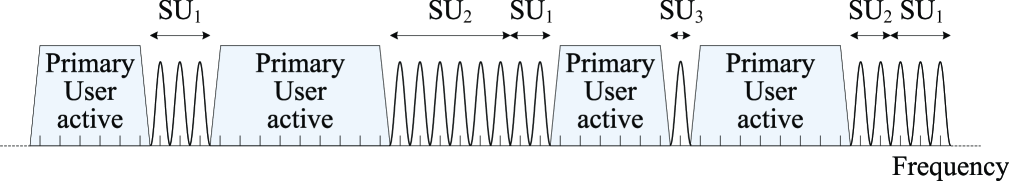
Fig. 1. Non-contiguous OFDM with Primary and Secondary Users (SUs), where the Secondary Users use non-contiguous channels that do not overlap with the Primary Users’ channels.

Under the basic model of Cognitive Radio Networks [2], Secondary Users (SUs) can use white spaces (also known as spectrum holes) that are not used by the Primary Users but must avoid interfering with active Primary Users (e.g., Figure 1). For example, the Primary and Secondary Users can be viewed as TV broadcasters and cellular operators using available TV bands [19]. Under this model, one assumes that when a transmission of a Primary User takes place, it occupies a predefined band. An SU may identify spectrum holes (not used by Primary or other Secondary Users) and can allocate its bandwidth among a number of subchannels, occupying a number of holes (not necessarily contiguous). This can be realized, for example, by employing a variant of Orthogonal Frequency-Division Multiplexing (OFDM) that is capable of deactivating sub-carriers which have the potential to cause interference to other users [16, 25, 29, 32, 31, 30] (such a non-contiguous OFDM scheme is shown in Figure 1).

The use of non-contiguous bandwidth blocks results in non-trivial behavior even for very simple scenarios. As an example, due to the dynamic use of the available spectrum holes and the arrivals and departures of SU bandwidth requests, SUs may need to transmit in a set of smaller and smaller holes. This will lead to a highly fragmented spectrum whose maintenance may require complex algorithmic solutions. Although the practical (physical layer) aspects of OFDM-based Dynamic Spectrum Access have been extensively studied recently, the use of fragmented (i.e., non-contiguous) spectrum introduces several new problems [21, 33, 31] that significantly differ from classical Medium Access Control (MAC) and fragmentation problems.

In this paper, we study the most basic theoretical model in which the spectrum is shared by SUs only. Those users have to transmit and receive data, and accordingly need some bandwidth for given amounts of time. Hence, bandwidth requests of SUs are characterized by a desired total bandwidth and the duration of a time interval over which it is needed. The data transmission can take place over a non-contiguous channel (i.e., a number of subchannels). Once a transmission terminates, some fragments (subchannels) are vacated, and therefore, gaps (spectrum holes/white spaces) develop randomly in both size and position.

When allocating a channel to a new SU request, it is being fragmented (in the frequency domain) into available gaps until the full requested bandwidth is provided. This process repeats itself, until the next request fails to fit into the available fragments. Figure 2 demonstrates the process of a transmission termination followed by the fragmentation of waiting bandwidth requests (more details about this example can be found in Section 2). We note that from a practical point of view, such a system can be viewed as a simplistic version of an OFDM-based access-point/base-station/spectrum-broker that tracks the available spectrum holes and allocates non-contiguous bandwidth blocks to SUs.

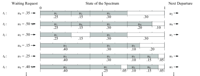
Fig. 2. An example of the admission and departure processes and the resulting spectrum fragmentation.

The main goal of the paper is to investigate the phenomena of fragmentation induced by spectrum allocation algorithms. For this purpose, we will ignore the particularities of techniques such as OFDM and make a couple of assumptions (for a complete system description, see Section 2): (i) the system operates at capacity and there is always a waiting bandwidth request; and (ii) the fragment size is not bounded from below. Making the first assumption allows us to study the effect of fragmentation in the worst case. Clearly, if there are idle periods, when there are no waiting requests, only departures occur and the fragmentation level of the system decreases during these periods. Similarly, the latter assumption allows us to study the system performance when artificial lower bounds on the fragment size are not imposed. This differs from OFDM-based systems in which a subcarrier has a given minimal bandwidth.

Main Results

At first glance, it seems that given assumption (ii) above, as time passes, the fragments used by bandwidth requests might well become progressively narrower and that the number of fragments grows without bound. Clearly, such an operation model cannot be supported by a realistic system (e.g., an OFDM-based system). However, our analytical and experimental results show that this is not the case.

In particular, under our model, a portion of the spectrum (represented by the interval $[0,1]$) is available for allocation to requests whose sizes are uniform on $(0,\alpha]$ ($0<\alpha\leq 1$). Once allocated, requests are satisfied (leave the system) after an exponential time. A stochastic model of channel fragmentation is investigated which includes the asymptotic behavior of the number $G(t)$ of gaps, $F(t)$ of fragments, and $R(t)$ of requests being served (also referred to as allocated channels). A Markovian description of this system is clearly more complicated than the vector $(G(t),F(t),R(t))$, since for each of the $R(t)$ channels, the location and size of each of its fragments should be included in such a description.

Let $(t_{n})$ be the sequence of request departure times. Our main result shows that the total number of gaps and fragments at these epochs has bounded exponential moments,

$$\sup_{n\geq 1}\mathbb{E}\left(e^{\eta(F(t_{n})+G(t_{n}))}\right)<+\infty,$$

for some $\eta>0$. It follows that the sum $F(t_{n})+G(t_{n})$ is strongly concentrated near the origin, indicating that, with high probability, low fragmentation of the spectrum holds under high traffic intensity. In our analysis, several basic ingredients are used: relations between the number of fragments and gaps in the spectrum; a drift relation of Lyapunov type for the total number of gaps, fragments, and requests (Proposition 1); a general inequality for Markov chains (Theorem 4); and a stability result of [22].

In addition to the analytical results, and in order to gain insight into the performance of the system, we present the results of an extensive simulation study. We show that although for a given maximum request size ($\alpha$), the number of fragments has a finite expected value, there is a linear relationship between 1/$\alpha$ and the expected number of fragments into which a request is divided. This indicates that when the requests are very small, they are also fragmented into a relatively large number of fragments. From a practical point of view, this implies that imposing a lower bound on the fragment size is important in order to reduce the complexity resulting from maintaining a channel heavily fragmented.

We show that different bandwidth allocation algorithms have significantly different performance in terms of the fragmentation occurring in the system. In particular, an algorithm (referred to as LFS) that allocates gaps in decreasing order of their sizes reduces the fragmentation by almost an order of magnitude compared to other algorithms. Interestingly, we also show that the number of fragments is distributed according to a Normal law with a relatively low mean value. Finally, we observe an unexpected reappearance of the 50% rule [23], according to which, on average the number of gaps (unoccupied fragments) is half the number of requests being served (this rule differs from the original 50% rule by Knuth [23] which is briefly discussed below).

Related Work

The areas of Dynamic Spectrum Access and Cognitive Radio Networks have been extensively studied (for a comprehensive review of previous work see [2, 1, 24, 26]). In particular, problems stemming from fragmented spectrum have been considered in [21, 33, 31]. In addition, several previous works focused on the technical aspects of channel fragmentation [15, 16, 29, 18, 32, 25, 30]. To the best of our knowledge, despite these recent efforts, the fragmentation problem considered in this paper has not been studied before.

Yet, the spectrum allocation problems described here can be characterized in the context of classical dynamic storage allocation problems of computers, see Knuth [23]. In that context, the term “spectrum” refers to the storage unit, “bandwidth” refers to storage, and “channel” refers to a region in storage containing a file. In the original storage model, fragmentation refers only to the gaps of unoccupied storage interspersed with intervals of occupied storage: files are not fragmented. The 50% rule was derived for this model and asserted that the number of gaps was approximately half the number of files when exact fits of files into gaps were rare. Our notion of fragmentation applies also to the files themselves, so our discovery that the 50% rule continued to apply was a surprising one at first. Note that, in terms of the storage application, our model corresponds well to linked-list allocation of files – channels allocated to requests are sets of linked, disjoint segments of storage allocated to specific file fragments. Our results provide a novel analysis for such systems, and have implications for the garbage-collection/defragmentation process in linked-list systems.

We note that studies of dynamic storage allocation have been around for some 40 years, and widely recognized as posing very challenging problems to both combinatorial and stochastic modeling and analysis. In particular, results of the type found in this paper, rigorous within stochastic models, seem to be quite new.

For a system without fragmentation, the early results of Kipnis and Robert [22] concern a stochastic analysis of the number of requests being served in the system. Fragmentation is not an issue in their case since request allocations can be moved when needed in order to put available space all together in one block. A major result in [22] applying to our model asserts the existence and uniqueness of an invariant measure for the number of requests. Explicit formulas for our system are hard to come by, but those in [22] for the maximal departure rate in special cases have provided useful checks on our experiments.

Organization of the Paper

The remainder of this paper is organized as follows. Section 2 describes the system, allocation algorithm, and the mathematical variables describing fragmentation. Section 3 presents simulation results that bring out the behavior of the system and the effects of fragmentation. Section 4 introduces some relations between the variables describing the fragmentation and a 50% limit law for the relation between the number of active channels and the number of gaps in the spectrum at departure times. Section 5 contains our main mathematical result, Theorem 2, which shows that the average value of the total number of fragments and gaps is bounded. Furthermore, in some cases, the existence of an equilibrium distribution is established in Theorem 3. Section 6 discusses algorithmic issues, such as changes in performance resulting from alternative algorithms for sequencing through the list of gaps when constructing a channel for a newly admitted request. Section 7 presents experiments suggesting that Normal approximations for the total number of fragments and gaps hold. Section 8 discusses the results and future research directions.

2. The Model

System Model

As mentioned above, we consider requests for bandwidth queued up waiting to be served, each of them identified with the amount of bandwidth required and a time telling how long it wants a channel with that total bandwidth. Channels are allocated to bandwidth requests on a FCFS (first-come-first-served) basis, subject to available bandwidth; the channels must remain fixed while active; they depart after varying delays, so gaps alternating with sequences of sub-channels (channel fragments) develop over time.

For convenience, we normalize the spectrum to the interval $[0,1]$, so all bandwidth requests are numbers in $[0,1]$. There is a queue of waiting requests that never empties. Assuming that the spectrum initially has no channels in use, the allocation process begins by allocating consecutive channels i.e., consecutive subintervals of [0,1], to requests whose sizes are $u_{1},u_{2},\ldots$ until a request whose size $u_{i},~{}i>1,$ is reached which exceeds available bandwidth, i.e.,

$$u_{1}+\cdots+u_{i-1}\leq 1<u_{1}+\cdots+u_{i}$$

All $i-1$ of the channels now begin their independent delays. Subsequent state transitions take place at departure epochs when the delays of currently allocated channels expire. At such epochs, all fragments of the departing channel are released. Suppose all requests up to $u_{j}$ have been allocated channels and a request $u_{i},~{}i\leq j$, departs, releasing its allocated channel. Then $u_{j+1},u_{j+2},\ldots$ are allocated their requested bandwidths until, once again, a request is encountered that asks for more bandwidth than is available. All channels then begin or continue their delays until the next departure. A standard rule for setting up a channel is to scan the spectrum, from one end to the other, with gaps of available bandwidth allocated to fragments of the new requested bandwidth until enough has been allocated to satisfy the entire request. The last gap used in satisfying a request is normally only partially used; the partial allocation in the last gap is left-justified in that gap. We refer to this scanning rule as Linear Scan.

An example is shown in Figure 2. Allocations for the first 8 user requests whose sizes are $u_{1},\cdots,u_{8}$ are shown, assuming that, at time 0, the spectrum is not in use. The requests with sizes $u_{1},$ $u_{2}$, and $u_{3}$ are the first to be allocated channels; $u_{4}$ must wait for a departure, since the first 4 request sizes sum to more than 1. The variables $t_{i}$ give the sequence of departure times of allocated requests. We see that the first occurrence of fragmentation takes place at the departure of $u_{2}$ and the subsequent admission of $u_{4}$; an initial fragment of $u_{4}$ is placed in the gap left by $u_{2}$ and a final fragment is placed after $u_{3}$. Note also that, even after $u_{2}$ and $u_{4}$ have departed, there is still not enough bandwidth for $u_{5}$. After the additional departure of $u_{1}$, both $u_{5}$ and $u_{6}$, but not $u_{7}$, can be allocated bandwidth.

In Section 6, we shall also evaluate two alternatives to the Linear Scan rule: a Circular Scan, by which each linear scan starts where the previous one left off, and a Largest-First Scan intended to further reduce fragmentation. Although these algorithms make different scans of the gap sequence, they are all alike in their treatment of the last gap occupied: the last fragment is left justified in the last gap. This is a key assumption, and it is very likely to hold in practice.

The allocation process described in this section contrasts with the classical model of dynamic storage allocation, in which each bandwidth request must be accommodated by a single, sufficiently large gap of available spectrum. However, the process does correspond closely to the linked-list model of dynamic storage allocation, in which an available-space list is maintained and files can be fragmented in accordance with this list. This paper also yields a novel stochastic analysis of such systems. Note that the assumption that there is always another request in queue models a system operating at capacity, where the departure rate, which is equal to the admission rate, is often called maximum throughput.

Notation, State Space, and Probability Model

We denote by $U$ the size of the request waiting to be allocated bandwidth, and by $U_{i}$ for $i\geq 1$ the size of the $i$th request behind it. Except in the proof of Theorem 3 in Section 5, we omit the dependency in time of these variables for the sake of notation. As mentioned in Section 2, we denote by $R(t)$ the number of channels (requests that are allocated bandwidth) at time $t$. $F(t)$ and $G(t)$ denote the number of fragments and gaps at time $t$. A Markovian description of this system is clearly more complicated than the vector $(G(t),F(t),R(t))$. Hence, we now define the state space of the fragmentation process. At a given state, we denote by $r$ the number of channels (requests to which bandwidth has been allocated) and by $s_{i}$ ($1\leq i\leq r$) the amount of bandwidth allocated to these requests. A state of the spectrum $[0,1]$ carries the information given by a sequence in which gaps alternate with sets of contiguous fragments:

Definition 1.

A state $x$ in the state space ${\mathcal{S}}$ of the fragmentation process is denoted by

$$x=(L_{1},\ldots,L_{r};u)$$

where $u$ is the size of (amount of bandwidth required by) the request waiting at the head of the queue and $L_{i},$ is the list of open subintervals of $[0,1]$ occupied by the fragments of the $i$-th channel. For $x$ to be admissible, the open intervals in $\cup_{i}L_{i}$ must be mutually disjoint, and, since the size of $u$ exceeds the bandwidth available, $u>1-\sum_{i}s_{i}$ has to hold.

Note that for a specific state, the size of the requests in the queue are denoted by $u$ and $u_{j},j\geq 1$ and the size of the channels (requests that are already allocated bandwidth) are denoted by $s_{i},1\leq i\leq r$.

Let $(X(t))$ be the process living in the state space $\mathcal{S}$. In the probability model used in this paper, the bandwidth requests ($U_{i}$) are independent random variables which are uniformly distributed on $(0,\alpha],0<\alpha\leq 1$, and request residence times are i.i.d. mean-$1$ exponentials. Under this probability model, $(X(t))$ is a Markov process on $\mathcal{S}$.

3. Experimental Results

In this section we describe an experimental study of the model described above. This serves two related roles. First, it brings out characteristics of the fragmentation process that need to be borne in mind in implementations, particularly where these characteristics show conditions (e.g., parameter settings) that must be avoided, if a system with fragmentation is to operate efficiently. The second role is that of experimental mathematics, in which results indicate where behavior might well be formalized and rigorously proved as a contribution to mathematical foundations. In the latter role, this section leads up to the next two sections, which formalize the stability of the fragmentation process.

The experiments were conducted with a discrete-event simulator written in C. In general, the tool is capable of simulating stochastic request arrival/departure processes. For this paper, however, the arrival process was effectively inoperative, since the interest here is behavior while the system is operating at capacity (i.e., at maximum throughput). Admissions are made whenever the waiting request fits into available spectrum, and once made the waiting request is immediately replaced by another with independent samples from the required-bandwidth and residence-time distributions. The admission process continues in this way, effectively simulating a queue that never empties, until no further admissions can be made and one or more departures need to occur. The excellent accuracy of the tool was established in tests against exact queueing results, and exact results from [22]. The verification details are omitted and can be found in Appendix A.

Recall that bandwidth requests are uniformly distributed on $(0,\alpha],0<\alpha\leq 1$. Hence, the principal parameter of the experimental model will be $\alpha$. The simulations of stationary behavior were most demanding, of course, for small $\alpha$. For every $\alpha$ value, $0.01\leq\alpha\leq 1$, $20$ million departure events were simulated starting in an empty state, with data collected for the last $10$ million events. For $0.001\leq\alpha\leq 0.01$, $100$ million departure events were processed and data collection was performed during the last $50$ million events.

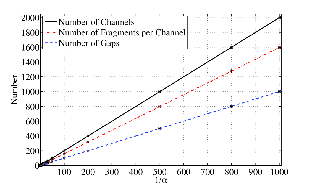
Fig. 3. Average numbers of channels, of gaps, and of fragments per channel.

The results for the average number of channels, the average number of gaps, and the average number of fragments per channel are shown in Figure 3. The curves are nearly linear in $1/\alpha$ (the errors in the linear fits are within the thickness of the printed lines). In particular, the asymptotic average number of channels in the spectrum is $2/\alpha$. When requests are large relative to the spectrum (i.e., for $\alpha>1/3$), the behavior is not given by functions quite so simple. As such cases are of less practical interest, we omit the relevant data due to space constraints.

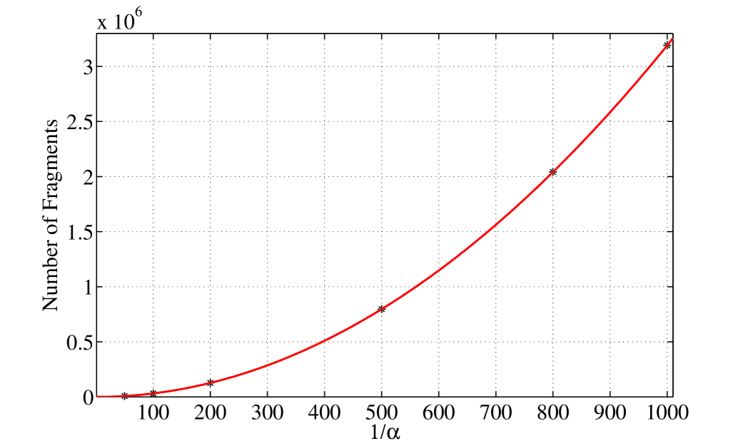
Fig. 4. Average total number of fragments vs. $1/\alpha$: a quadratic fit.

The asymptotic linear growth of the average number of channels as a function of channel size is obvious, but the linearity of the other two measures is not so obvious. A closer look shows that the average number of gaps is almost exactly one half the average number of channels for even relatively small $1/\alpha$. This is an unexpected version of Knuth’s 50% rule for dynamic storage allocation. We return to this behavior in the next section, where we prove a 50% limit law. The linear growth of the average number of fragments per channel may also be unexpected at first glance: the fragmentation of channels increases as the average channel size decreases. This linear growth implies the quadratic growth of the average total number of fragments plotted in Figure 4 (the accuracy of the fit is as before: the error is within the thickness of the printed lines).

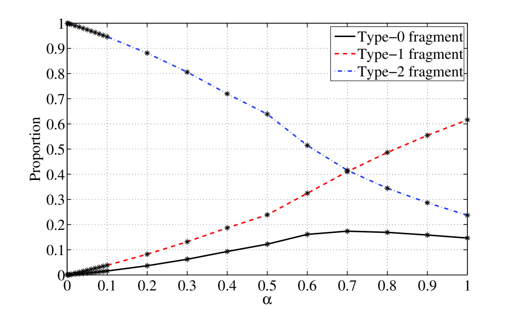
Fig. 5. Percentage of type-$i$ fragments.

The analysis in the later sections will focus largely on tracking fragment types defined as follows: a fragment is of type-$i$, if it is adjacent to $0,1,~{}{\rm or}~{}2$ fragments. It can be seen in Figure 5 that for small $\alpha$, more than 90% of the fragments are type-$2$ fragments. In addition, clearly, the number of type-$0$ and type-$1$ fragments is a function of the number of gaps. These observations and the results illustrated in Figures 3 and 4 indicate that, even for relatively small $1/\alpha$, the average total number of type-$0$ and type-$1$ fragments grows linearly in $1/\alpha$, but the average number of type-$2$ fragments grows quadratically.

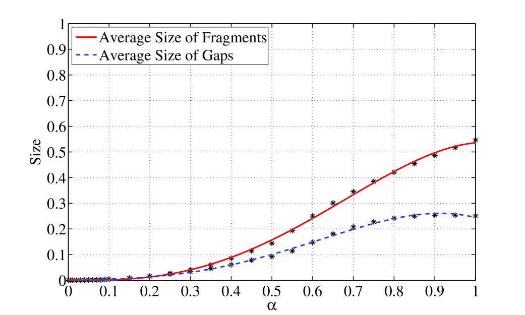
(a) $0\leq\alpha\leq 1$

(b) $0\leq\alpha\leq 0.1$

Fig. 6. Average sizes of fragments and gaps.

Figure 6 compares the average gap and fragment sizes. As might be expected, for relatively small $\alpha$, they are close to each other. The relation holds even for moderately large $\alpha$, although for $\alpha$ rather close to 1, the difference amounts to about a factor of 2. With this property and the 50% rule suggested by Figure 3, the linear growth in the number of fragments per channel (shown in Figure 3) is easily explained for moderately small $\alpha$ in the following way.

As mentioned above, for moderately small $\alpha$, the number of channels is approximately $2/\alpha$ (i.e., the spectrum size divided by the average request size). Due to the 50% rule, the number of gaps is roughly $1/\alpha$. At any time, the total size of the gaps is at most $\alpha$, since there is a request waiting for departures whose requested bandwidth exceeds that total size of gaps. Therefore, at most $\alpha$ available bandwidth is spread among $1/\alpha$ gaps, giving an average gap size on the order of $\alpha^{2}$. The average fragment size is at most (and indeed very close to) the average gap size. The fragments must occupy at least $1-\alpha$ of the spectrum (since, as mentioned above, at most a fraction $\alpha$ of the spectrum is devoted to gaps). Thus, the number of fragments must be on the order of $1/\alpha^{2}$, and so the average number of fragments per channel must be on the order of (in particular, linear in) $1/\alpha$. As $\alpha\rightarrow 0$, the asymptotics of these estimates become more precise.

4. Numbers of Fragments and Gaps

As mentioned in Section 2, under our probability model, $(X(t))$ (the process living in the state space $\mathcal{S}$) is a Markov process on $\mathcal{S}$. In this section, we obtain analytical results regarding the number of fragments and gaps under this process. We begin by formally defining the fragment types which were discussed in Section 3.

Definition 2.

For $i=$ 0,1, or 2, a fragment is said to be of type $i$ if it touches exactly $i$ other fragments. $N_{i}(t)$ denotes the number of type $i$ fragments at time $t$, so that $F(t)=N_{0}(t)+N_{1}(t)+N_{2}(t)$ is the total number of fragments.

Let $\sigma(t)$ denotes the sum of the number of fragments and gaps,

(1) $$\sigma(t)=F(t)+G(t).$$

The number $G(t)$ of gaps and the numbers of fragment types are related as follows.

Lemma 1.

With probability $1$,

(2) $$G(t)=N_{0}(t)+\frac{1}{2}N_{1}(t)+I(t)$$

For any $t\geq 0$, where $I(t)=1$, if there is a gap starting at the origin, and 0 otherwise.

Proof.

Each gap, except for boundary gaps starting at 0 or ending at 1, separates two fragments. Two gaps surround a type-0 fragment not touching the origin, only one touches a type-1 fragment not touching the origin, and none touch a type-2 fragment, so the gaps strictly inside $(0,1)$ are double-counted in $2N_{0}(t)+N_{1}(t)$. Gaps at the boundaries are counted only once in this expression, so if there are gaps touching each boundary, 2 must be added to $2N_{0}(t)+N_{1}(t)$ to produce a double count of all gaps. Then $N_{0}(t)+N_{1}(t)/2+1$ counts the gaps as called for by the lemma.

With probability $1$, a gap always touches the boundary at $1$, so the only case left to consider is the absence of a gap touching the origin. In this case, there is a type-0 or type-1 fragment touching the origin, and so a nonexistent gap has been counted in $2N_{0}(t)+N_{1}(t)$. This over-count cancels the under-count of the gap touching 1, and so no correction term is needed, i.e., $N_{0}(t)+N_{1}(t)/2$ counts all gaps as stated in the lemma. ∎

Definition 3.

Let $(t_{k})$ denote the sequence of departure times, let $D_{i}(t_{k})$ denote the number of type $i$ fragments in the channel leaving at time $t_{k}$, and let $A(t_{k})$ denote the number of requests admitted to the spectrum at time $t_{k}$. Finally, define the drift in the total number of fragments and gaps:

(3) $$\Delta\sigma(t_{k})\stackrel{{\scriptstyle\text{def}}}{{=}}\sigma(t_{k})-\sigma(t_{k-1}).$$

The following lemma is the basis of the stability analysis of $\sigma(t)$ in Section 5, and the 50% rule proved later in this section.

Lemma 2.

With probability $1$, the departure at $t_{k}$ creates the following change in the total number of fragments and gaps:

(4) $$\Delta\sigma(t_{k})=A(t_{k})-2D_{0}(t_{k})-D_{1}(t_{k})+J(t_{k}),~{}~{}k\geq 1$$

with $t_{0}=0$, and $J(t_{k})=1$, if a fragment starting at the origin is in the departing channel, and 0 otherwise.

Proof.

With probability 1, each new channel allocation covers completely every gap it is allocated, except for the last one, which is only partially covered. Thus, with probability 1, each new channel allocation changes gaps to fragments, except for the last gap which is changed to a fragment plus a gap; this adds one to $\sigma(t_{k-1})$ for each admission, which accounts for the total of $A(t_{k})$ in (4).

Two fragments of the same channel can not be contiguous, so it is correct to add up the changes created by departing fragments, with each being treated separately. Suppose first that there is no fragment $(0,b)$ against the origin. Then for every type-0 fragment in the departing channel, two gaps and a fragment are replaced by a single gap for a net decrease of two, and for every departing type-1 fragment, a gap and a fragment are replaced by a single gap for a net reduction of one. This gives the reduction of $2D_{0}(t_{k})+D_{1}(t_{k})$ appearing in (4). If there is a fragment $(0,b)$, it must be of type 0 or 1; if it is of type 0, then its departure gives a decrease of one; if it is of type 1, its departure has no effect. Each of these contributions is one less than it would be were the fragment not touching the origin. There can only be one such fragment, so the correction shown in $J(t_{k})$ for a fragment $(0,b)$ follows. ∎

We will denote by $G^{-}(t_{k})$ the total number of gaps just after the $k$-th departure, but before new admissions, if any, are made. Note that if we remove $A(t_{k})$ from the right-hand side of (4) and add back the total number of departing fragments at $t_{k}$, i.e., $D_{0}(t_{k})+D_{1}(t_{k})+D_{2}(t_{k}),$ we get the number of gaps available to admissions at the $k$-th departure:

(5) $$G^{-}(t_{k})=G(t_{k-1})-D_{0}(t_{k})+D_{2}(t_{k})+J(t_{k})$$

with $J(t_{k})=1$, if there is a departing fragment $(0,b)$, and $0$ otherwise.

Knuth’s widely known 50% rule appears in a very different context than the model here, so it is difficult to anticipate the apparent fact that it also holds for our fragmentation model. However, one can argue a similar result assuming only that the fragmentation process has a stationary distribution. The result is given below as an expected value of a ratio, rather than a ratio of expected values.

Theorem 1.

Assume that the fragmentation process at departure epochs $t_{k}$ has the stationary distribution $\pi_{\alpha}$, then as $\alpha\rightarrow 0,$

$$\mathbb{E}_{\pi_{\alpha}}\left({G(t_{k})\over R(t_{k})}\right)\sim\frac{1}{2}$$

Proof.

In the stationary regime, one has, by Lemma 2,

$$\mathbb{E}_{\pi_{\alpha}}[\sigma(t_{k})-\sigma(t_{k-1})] =$$

$$\mathbb{E}_{\pi_{\alpha}}[A(t_{k})-2D_{0}(t_{k})-D_{1}(t_{k})+J(t_{k})] =0,$$

and to balance departure and admission rates, we must have $\mathbb{E}_{\pi_{\alpha}}A(t_{k})=1$. Thus, we can write

(6) $$\mathbb{E}_{\pi_{\alpha}}[2D_{0}(t_{k})+D_{1}(t_{k})-J(t_{k})]=1.$$

Now for a state $x$ at time $t_{k}$ having $r$ channels and $N_{i}(t_{k})$ type-$i$ ($i=0,1,2$) fragments, we have from Lemma 1

$$\mathbb{E}_{x}[2D_{0}(t_{k})+D_{1}(t_{k})-J(t_{k})] =(2N_{0}(t_{k})+N_{1}(t_{k}))/r-\mathbb{E}_{x}[J(t_{k})]$$

$$=2[G(t_{k})-I(t_{k})]/r-\mathbb{E}_{x}[J(t_{k})]=2G(t_{k})/r+O\left(1/r\right)$$

Thus, dropping the $O(1/r)$ term that tends to 0 with $\alpha$ uniformly in $x$, the expectation in (6) proves the theorem. ∎

5. Stability Results

This section establishes that the average total number of fragments and gaps remains bounded and that, for certain distributions of request sizes, ergodicity holds. The analysis leads to the two following results. Recall that $(t_{n})$ is the sequence of departure times ($t_{0}=0$) and $\sigma(t)=F(t)+G(t)$, defined in (1), is the total number of fragments and gaps.

Theorem 2.

There exists some $\eta>0$ such that, for any initial state $x\in\mathcal{S}$,

(7) $$\sup_{n\geq 1}\mathbb{E}_{x}\left(e^{\eta\sigma(t_{n})}\right)<+\infty.$$

Clearly, this implies that for any initial state $x\in\mathcal{S}$, the sequence $(\mathbb{E}_{x}(\sigma(t_{n})),n\geq 0)$ is bounded. With an additional assumption on the distribution of the request size, a stronger stability result can be proved.

Theorem 3.

When $\alpha>1/2$, the process $(X(t))$ is positive Harris recurrent; in particular, it has a unique stationary distribution.

A criterion for finite exponential moments using a Lyapunov function is established next. Then, we provide some estimates of the drift of the number of fragments between departures which will show us how to construct a Lyapunov function. After constructing this function, we will be in position to prove the boundedness of exponential moments.

A Criterion for Finite Exponential Moments

Before stating the main result, some results on Markov chains are needed. In the sequel, $\leq_{st}$ refers to stochastic ordering, i.e., $V\leq_{st}Z$ means that $\mathbb{E}(f(V))\leq\mathbb{E}(f(Z))$ for any increasing function $f$. For reasons that will become clear in Lemma 5, the following lemma focuses on admissions at $4$ consecutive departure times. Recall that $(U_{i},i\geq 1)$ are the sizes of the requests waiting to be allocated bandwidth (after the first one $U$), which are assumed to i.i.d.

Lemma 3.

The random variable $A(t_{1})+\cdots+A(t_{4})$ is stochastically dominated by a random variable $Z$ such that $\mathbb{E}(e^{\lambda Z})<+\infty$ for some $\lambda>0$.

Proof.

It is clear that $A(t_{1})\leq Z+1$ where

$$Z=1+\inf\{n\geq 1:U_{1}+\cdots+U_{n}\geq 1\}.$$

The Markov inequality shows that for any $z\geq 0$,

$$\mathbb{P}(Z\geq z+1)=\mathbb{P}(U_{1}+\cdots+U_{z}\leq 1)\leq e\left(\mathbb{E}\left(e^{-U_{1}}\right)\right)^{z}$$

and so $\mathbb{E}(e^{\eta Z})$ is finite for $\eta>0$ small enough. From this observation, it is not difficult to extend the result to $A(t_{1})+\cdots+A(t_{4})$ instead of just $A(t_{1})$. ∎

This lemma shows in particular that

$$\xi\stackrel{{\scriptstyle\text{def}}}{{=}}\sup_{i\geq 1}\sup_{x\in\mathcal{S}}\mathbb{E}_{x}(A(t_{i}))<+\infty.$$

is well-defined; this constant will be used repeatedly throughout the rest of the analysis. The proof of the following lemma is standard, and therefore, omitted.

Lemma 4.

Let $Z\geq 0$ be a positive, real-valued random variable such that $\mathbb{E}(e^{\lambda Z})<+\infty$ for some $\lambda>0$, and define $c=\lambda^{-2}\mathbb{E}(e^{\lambda Z}-1-\lambda Z).$ Then for any $0\leq\varepsilon\leq\lambda$ and any real-valued random variable $V$ such that $V\leq_{\text{st}}Z$, we have $\mathbb{E}\left(e^{\varepsilon V}\right)\leq 1+\varepsilon\mathbb{E}(V)+\varepsilon^{2}c.$

The following result is closely related to result of Hajek [17]. The proof can be found in Appendix B.

Theorem 4.

Let $(Y_{k})$ be a discrete-time, continuous state-space Markov chain such that for some function $f\geq 0$, there exist $K,\gamma>0$ such that for any initial state $y$ with $f(y)>K$, $\mathbb{E}_{y}(f(Y_{1})-f(Y_{0}))\leq-\gamma.$ Assume that there exists a random variable $Z$ such that for any initial state $y$, $Z$ dominates stochastically the random variable $f(Y_{1})-f(Y_{0})$ under $\mathbb{P}_{y}$. Assume finally that $\mathbb{E}(e^{\lambda Z})<+\infty$ for some $\lambda>0$. Then there exist $\eta>0$ and $0\leq C<+\infty$ such that for any initial state $y$,

$$\sup_{n\geq 1}\mathbb{E}_{y}\left(e^{\eta f(Y_{n})}\right)\leq e^{\eta f(y)}+C.$$

Theorem 4 will be applied to the Markov chain $(X(t_{4n}))$ with a function $f$ of the form $\sigma_{\kappa}=\sigma+\kappa r$ for some $\kappa>0$ suitably chosen. $(X(t_{4n}))$ is not the most natural choice at first glance, but it appears to be needed because of the complexity of the state space.

It is clear that $\sigma(t_{1})-\sigma(t_{0})\leq A(t_{1})+1$, so that

$$\sigma_{\kappa}(t_{4})-\sigma_{\kappa}(t_{0})\leq(\kappa+1)(A(t_{1})+\cdots+A(t_{4}))+4$$

and therefore, by Lemma 3, $\sigma_{\kappa}(t_{4})-\sigma_{\kappa}(t_{0})$ is stochastically dominated by some random variable $Z$ with an exponential moment. Therefore, one has to establish a negative drift relation for $\sigma_{\kappa}(t_{4})-\sigma_{\kappa}(t_{0})$. This is the purpose of the following two subsections.

Evolution of the Number of Fragments

Recall that $x\in\mathcal{S}$, the initial state of the system, has $r$ active channels, and define the total available gap size $h=1-(s_{1}{+}\cdots{+}s_{r}).$ Time $0$ referring to the initial state $x$ will usually be omitted; e.g., $\sigma(0),F(0),G(0),\ldots$ will be simplified to $\sigma,F,G,\ldots$. Recall that $\Delta\sigma(t_{n})$ is defined in (3) as $\sigma(t_{n})-\sigma(t_{n-1}).$

Lemma 5.

Fix $0<\varepsilon<1$ and $0<\eta<1/2$, and let $x\in\mathcal{S}$ be an initial state such that $\sigma=G+F\geq 2K+1$ for some fixed $K\geq 0$.

Then $F=N_{0}+N_{1}+N_{2}\geq K$, and

1. If $r=1$, then $\mathbb{E}_{x}(\Delta\sigma(t_{1}))\leq\xi-K$.

1. If $r>1$ and $N_{0}+N_{1}\geq\varepsilon K$, then

   $$\mathbb{E}_{x}(\Delta\sigma(t_{1}))\leq\xi+1-\frac{\varepsilon K}{r}.$$

Assume in the remaining cases that $r>1$, define $K^{\prime}=K\big{(}(1-\varepsilon)/r-\varepsilon\big{)}^{+}$, and let $i^{*}\in\{1,\ldots,r\}$ index a channel $L_{i^{*}}$ in $x$ with the most type-$2$ fragments.

1. If $N_{0}+N_{1}\leq\varepsilon K$ and $u>h+s_{i^{*}}$, then

   (8) $$\mathbb{E}_{x}(\Delta\sigma(t_{2}))\leq\xi+2-\frac{K^{\prime}}{r(r-1)}.$$

2. If $N_{0}+N_{1}\leq\varepsilon K$, $u<h+s_{i^{*}}$ and $h+s_{i^{*}}<\eta\alpha$, then

   (9) $$\mathbb{E}_{x}(\Delta\sigma(t_{3}))\leq\xi+2-\frac{(1-\eta)K^{\prime}}{r^{2}(r-1)}.$$

3. If $N_{0}+N_{1}\leq\varepsilon K$, $u<h+s_{i^{*}}$ and $\eta\alpha<h+s_{i^{*}}$, then there exists a $\gamma(\eta)>0$ such that

   (10) $$\mathbb{E}_{x}(\Delta\sigma(t_{4}))\leq\xi+2-\frac{\gamma(\eta)K^{\prime}}{r^{5}}.$$

It follows that there exists a $\overline{\xi}>0$ and a function $\psi(r)>0$ such that for any $x$ with $\sigma\geq 2K+1$,

(11) $$\mathbb{E}_{x}(\sigma(t_{4})-\sigma)\leq\overline{\xi}-K\psi(r).$$

Proof.

As is readily verified, $G\leq F+1$, so $2K+1\leq\sigma=F+G\leq 2F+1$, and hence $F\geq K$ as claimed. In what follows, we use repeatedly the two following simple facts:

(12) $$\mathbb{E}_{x}\left(D_{0}(t_{1})+D_{1}(t_{1})\right)=(N_{0}+N_{1})/r,$$

and by Lemma 1,

(13) $$G\geq K\Rightarrow N_{0}+N_{1}\geq K-1.$$

— First case: $r=1$. Then, right after the only channel initially present leaves, there is no channel allocated bandwidth, and therefore, $\sigma(t_{1})=A(t_{1})$. Note that $r=1$ is only possible when $\alpha>1/2$, and in this case the possibility for a channel to be alone is crucial in the proof of the Harris recurrence stated in Theorem 3.

— Second case: $r>1$, $N_{0}+N_{1}\geq\varepsilon K$. Then the inequality follows from (4):

$$\mathbb{E}_{x}(\Delta\sigma(t_{1}))\leq\xi+1-\mathbb{E}_{x}(D_{0}(t_{1})+D_{1}(t_{1}))=\xi+1-\frac{N_{0}+N_{1}}{r}\leq\xi+1-\frac{\varepsilon K}{r}.$$

In the 3 remaining cases, let $N^{*}_{j}$ denote the number of type-$j$ fragments in any channel $i^{*}$ which has the most type-$2$ fragments. If $N_{0}+N_{1}\leq\varepsilon K$, then since $F\geq K$, necessarily $N_{2}\geq(1-\varepsilon)K$ and $N^{*}_{2}\geq(1-\varepsilon)K/r.$ Define the event $D^{*}=\{\text{channel }L_{i^{*}}\text{ leaves at }t_{1}\}$ and recall that $G^{-}$ denotes the number of gaps right after $L_{i^{*}}$ leaves but before new admissions, if any, are made. It follows from (5) that $G^{-}\geq K^{\prime}$ in the event $D^{*}$, since

$$G^{-}=G-N^{*}_{0}+N^{*}_{1}+J(t_{1})\geq\left(-\varepsilon K+(1-\varepsilon)K/r\right)^{+}=K^{\prime}.$$

The remaining analysis tacitly assumes that $r>1$, that $N_{0}+N_{1}\leq\varepsilon K$ and that the channel $L_{i^{*}}$ leaves at $t_{1}$.

— Third case: $u>h+s_{i^{*}}$. Then $A(t_{1})=0$, since when $L_{i^{*}}$ leaves it does not provide enough additional bandwidth for $U$. In particular, $R(t_{1})=r-1$ and $G(t_{1})=G^{-}\geq K^{\prime}$, and so

$$\mathbb{E}_{x}(\Delta\sigma(t_{2}))\leq\xi+1-\mathbb{E}_{x}(D_{0}(t_{2})+D_{1}(t_{2});D^{*}).$$

The strong Markov property makes it possible to lower-bound this last term.

$$\mathbb{E}_{x}(D_{0}(t_{2})+D_{1}(t_{2});D^{*})=\mathbb{E}_{x}(\mathbb{E}_{X(t_{1})}(D_{0}(t_{1})+D_{1}(t_{1}));D^{*})\\ =\mathbb{E}_{x}\left(\frac{(N_{1}+N_{2})(t_{1})}{R(t_{1})};D^{*}\right)\geq\frac{K^{\prime}-1}{r-1}\mathbb{P}_{x}(D^{*})=\frac{K^{\prime}-1}{r(r-1)}$$

and therefore, $\mathbb{E}_{x}(\Delta\sigma(t_{2}))\leq\xi+2-K^{\prime}/(r(r-1))$.

— Fourth case: $u<h+s_{i^{*}}<\eta\alpha$. In this case $U$ is admitted at $t_{1}$. Thus it makes sense to define the event

$$E_{4}=D^{*}\,\cap\,\{U\text{ leaves at }t_{2}\text{ and }U_{1}>\eta\alpha\}.$$

Then as before

$$\mathbb{E}_{x}(\Delta\sigma(t_{3}))\leq\xi+1-\mathbb{E}_{x}(D_{0}(t_{3})+D_{1}(t_{3});E_{4}).$$

In the event $E_{4}$, $U$ is admitted at $t_{1}$ and leaves at $t_{2}$, while $U_{1}$ stays blocked at $t_{1}$ and $t_{2}$, so that $G(t_{2})=G^{-}\geq K^{\prime}$ and $R(t_{2})=r-1$. Hence as in the second case,

$$\mathbb{E}_{x}(D_{0}(t_{3})+D_{1}(t_{3});E_{4})\geq\frac{K^{\prime}-1}{r-1}\mathbb{P}_{x}(E_{4})\geq\frac{(1-\eta)K^{\prime}}{r^{2}(r-1)}-1$$

since $\mathbb{P}_{x}(E_{4})=(1-\eta)/r^{2}$. Thus (9) holds.

— Fifth case: $u<h+s_{i^{*}}$ and $\eta\alpha<h+s_{i^{*}}$. Again, $U$ is admitted at $t_{1}$. Letting $U_{i}$ denote the sizes of the requests behind $U$, define the event

$$B=\{U_{i}<\eta\alpha,\ i=1,\ldots,\tau\text{ and }U_{\tau+1}>2\eta\alpha\}$$

with $\tau=\inf\{n\geq 0:U_{1}+\cdots+U_{n}>h+s_{i^{*}}-\eta\alpha\}$ and $E_{5}^{\prime}=D^{*}\,\cap\,B\,\cap\,\{U\text{ leaves at }t_{2}\}.$ It is readily verified that $1\leq\tau<+\infty$ almost surely. Moreover, one has in $E_{5}^{\prime}$

$$0<h^{*}\stackrel{{\scriptstyle\text{def}}}{{=}}h+s_{i^{*}}-(U_{1}+\cdots+U_{\tau})<\eta\alpha<U_{\tau+1}.$$

This means that at $t_{2}$, exactly $\tau$ new requests $U_{1},\ldots,U_{\tau}$ have been admitted, and $U_{\tau+1}$ is blocked. Moreover, for any $i\in\{1,\ldots,\tau\}$, one has $h^{*}+U_{i}<2\eta\alpha<U_{\tau+1},$ so that if one of the $\tau$ channels allocated to the $(U_{i})$ leaves, $U_{\tau+1}$ remains blocked.

When $L_{i^{*}}$ left, there were $G^{-}\geq K^{\prime}$ gaps; in the remainder of the analysis, we call an initial gap a gap present right after $L_{i^{*}}$ left. After $L_{i^{*}}$ left, $U$ and $A(t_{1})-1$ new requests were admitted, and then $U$ left and $A(t_{2})$ new requests were admitted at $t_{2}$. Thus, at $t_{2}$, each initial gap is in either of two states: either it is completely filled, or it is still a gap, i.e., it has not been filled completely. Let $k$ be the number of initial gaps completely filled at $t_{2}$, and let $k^{\prime}=G^{-}-k$: then $k+k^{\prime}=G^{-}\geq K^{\prime}.$ In each initial gap completely covered at $t_{2}$, there is at least one type-$2$ fragment of one of the $\tau$ new channels. Therefore, $N_{1,2}+N_{2,2}+\cdots+N_{\tau,2}\geq k$ with $N_{i,2}$ the number of type-$2$ fragments of the channel corresponding to $U$. In particular there is a channel $L_{j^{*}},~{}j^{*}\in\{1,\ldots,\tau\}$ with at least the average $k/\tau$ of type-$2$ fragments: $N_{j^{*},2}\geq k/\tau$. Define finally the event $E_{5}=E_{5}^{\prime}\,\cap\,\{L_{j^{*}}\text{ leaves at }t_{3}\}.$ Since $h^{*}+U_{j^{*}}<U_{\tau+1}$, then $U_{\tau+1}$ remains blocked at $t_{3}$ when $E_{5}$ occurs, and therefore (note that when $j^{*}$ leaves, some gaps may merge, but not two initial gaps),

$$G(t_{3})\geq N_{j^{*},2}+k^{\prime}\geq k/\tau+k^{\prime}\geq(k+k^{\prime})/\tau\geq K^{\prime}/\tau.$$

Now we proceed as before, to obtain

$$\mathbb{E}_{x}(\Delta\sigma(t_{4}))\leq\xi+1-\mathbb{E}_{x}(D_{0}(t_{4})+D_{1}(t_{4});E_{5})$$

and, using the Markov property at time $t_{3}$,

$$\mathbb{E}_{x}(D_{0}(t_{4})+D_{1}(t_{4});E_{5})=\mathbb{E}_{x}(\mathbb{E}_{X(t_{3})}(D_{0}(t_{1})+D_{1}(t_{1}));E_{5})\\ =\mathbb{E}_{x}\left(\frac{(N_{0}+N_{2})(t_{3})}{R(t_{3})};E_{5}\right)\geq\mathbb{E}_{x}\left(\frac{(K^{\prime}/\tau-1)^{+}}{r+\tau-2};E_{5}\right)$$

since $R(t_{3})=r+\tau-2$ in $E_{5}$. The same kind of reasoning as before then leads to

$$\mathbb{E}_{x}\left(\frac{(K^{\prime}/\tau-1)^{+}}{r+\tau-2};E_{5}\right)\geq\frac{K^{\prime}}{r^{5}}f(\eta,h+s_{i^{*}}-\alpha\eta)-1$$

with the function $f(\eta,\cdot)$ defined for $y>0$ by

$$f(\eta,y)=\mathbb{E}\left((1+\tau(y))^{-5};B(\eta,y)\right)$$

with $\tau(y)=\inf\{n\geq 1:U_{1}+\cdots+U_{n}\geq y\}$ and

$$B(\eta,y)=\{U_{i}<\eta\alpha,i=1,\ldots,\tau(y)\text{ and }U_{\tau(y)+1}>2\eta\alpha\}.$$

It is not difficult to show that $\gamma(\eta)=\inf_{0<y<1}f(\eta,y)>0$ which then gives the result.

It remains to prove (11). One only needs to assemble the various bounds, taking into account that $\mathbb{E}_{x}(\Delta\sigma(t_{i}))\leq\xi+1$ for any $x\in\mathcal{S}$ and $i\geq 0$, to arrive at 4 separate bounds on $\mathbb{E}_{x}(\sigma(t_{4})-\sigma)$. For example, using the former bound for the first two terms and the last term of $\mathbb{E}_{x}(\sigma(t_{4})-\sigma)=\sum_{1\leq i\leq 4}\mathbb{E}_{x}\Delta\sigma(t_{i})$ and then the bound in (9) for the third term, we get that one of the 4 bounds, which applies when $x$ satisfies the inequalities of the fourth case, is

$$\mathbb{E}_{x}(\sigma(t_{4})-\sigma)\leq 4\xi+5-\frac{(1-\eta)K^{\prime}}{r^{5}}$$

Computing the minimum over these bounds with $\eta=1/4$ and $\varepsilon=1/r^{2}$, one obtains (11) after setting $\overline{\xi}=4\xi+5$ and

$$\psi(r)=\frac{\varphi(r)}{r^{6}}\times((1-\eta)\wedge\gamma)$$

with $\varphi(r)=1-2r^{-2}$. This concludes the proof. ∎

We turn now to the case where $r$ is large. In this case, the negative drift comes from the fact that, except perhaps at $t_{1}$, with high probability there is no admission at a departure, since the channel that leaves is small with high probability. However, we see in (4) that this is not enough for $\sigma$ to decay, for one would need at least one type-$0$ or type-$1$ fragment to leave as well, and it can be the case that most fragments are of type-$2$. The second term of the Lyapunov function allows us to get around this problem. Since the variation $\Delta R(t_{k})$ in the number of channels at a departure is exactly equal to $A(t_{k})-1$, one readily gets that

$$\sigma_{\kappa}(t_{4})-\sigma_{\kappa}=(\sigma(t_{4})-\sigma)+\kappa(A(t_{1})+\cdots+A(t_{4})-4).$$

In particular, if $x\in\mathcal{S}$ is such that $\sigma\geq 2K+1$ and $r\leq K_{r}$, then (from now on, we assume without loss of generality that the function $\psi$ given by (11) in Lemma 5 is decreasing)

$$\mathbb{E}_{x}(\sigma_{\kappa}(t_{4})-\sigma_{\kappa})\leq\overline{\xi}-K\psi(K_{r})+4\kappa(\xi-1)$$

whereas if $r\geq K_{r}$,

$$\mathbb{E}_{x}(\sigma_{\kappa}(t_{4})-\sigma_{\kappa})\leq 4(\xi+1)+\kappa\mathbb{E}_{x}(r(t_{4})-r)$$

and so we see that we only need to control $\mathbb{E}_{x}(r(t_{4})-r)$ for $r$ large.

Lemma 6.

There exist $K_{r},\gamma_{r}>0$ such that if $x\in\mathcal{S}$ is such that $r\geq K_{r}$, then $\mathbb{E}_{x}(r(t_{4})-r)\leq-\gamma_{r}.$

Proof.

Since the technical difficulty of the proof of this inequality is similar to that of the above proof, we need only give a sketch of it. From $s_{1}+\cdots s_{r}=1-h\leq 1$ one gets $\#\{i:s_{i}\geq\gamma\}\leq 1/\gamma$, and therefore, $\mathbb{P}_{x}(s_{i_{1}}\geq 1/\sqrt{r})\leq 1/\sqrt{r}$ with $L_{i_{1}}$, $i_{1}\in\{1,\ldots,r\},$ the channel that leaves at $t_{1}$. Thus, when $r$ is large, with high probability a small channel leaves.

If $h-u$ is away from $\alpha$, then the event $\{u_{1}>h-u+s_{i_{1}}+\cdots+s_{i_{4}}\}$ (with $i_{k}$ defined similarly) has high probability, and in this event $A(t_{1})+\cdots+A(t_{4})\leq 1$. If in contrast $h-u$ is large, then with high probability $U_{1}$ is admitted and with high probability $h-u-U_{1}$ is away from $\alpha$; hence we can do the same again, and get that, with high probability, $A(t_{1})+\cdots+A(t_{4})\leq 2$. The lemma is proved. ∎

Construction of a Lyapunov Function

For $\kappa>0$, one defines, for an initial state $x\in\mathcal{S}$ of the system, $\sigma_{\kappa}\stackrel{{\scriptstyle\text{def}}}{{=}}\sigma+\kappa\,r,$ where $r$ is the number of channels allocated in $x$ and $\sigma=F+G$ is the sum of the number of fragments and gaps in $x$.

Proposition 1.

(Lyapunov function inequality) There exist $\kappa$ and $K>0$ such that if $x\in\mathcal{S}$ is such that $\sigma_{\kappa}\geq K$, then $\mathbb{E}_{x}(\sigma_{\kappa}(t_{4})-\sigma_{\kappa})\leq-1.$

Proof.

Let $K_{r}$ and $\gamma_{r}$ be as in Lemma 6, and take $\kappa$ and $K$ as follows:

$$\kappa=\frac{4\xi+5}{\gamma_{r}}\ \text{ and }\ K=\frac{8\xi+2\overline{\xi}+2}{\psi(K_{r})}+\kappa K_{r}+1.$$

Assume that $\sigma_{\kappa}\geq K$. If $r\geq K_{r}$, then

$$\mathbb{E}_{x}(\sigma_{\kappa}(t_{4})-\sigma_{\kappa})\leq 4(\xi+1)-\kappa\gamma_{r}=-1.$$

Otherwise, $r\leq K_{r}$, and since $\sigma_{\kappa}\geq K$, this necessarily gives $\sigma\geq K-\kappa K_{r}=2\hat{K}+1$ with $\hat{K}=(K-\kappa K_{r}-1)/2$. Thus,

$$\mathbb{E}_{x}(\sigma_{\kappa}(t_{4})-\sigma_{\kappa})\leq\overline{\xi}-\hat{K}\psi(K_{r})+4\xi=-1$$

and the proposition follows. ∎

Proof of Theorem 2

Theorem 4 and Lemma 3 applied to the Markov chain $(X(t_{4n})$, $n\geq 0),$ and the function $\sigma_{\kappa}$ show that for some $\eta>0$ and some constant $0\leq C<+\infty$,

$$\sup_{n\geq 0}\mathbb{E}_{x}\left(e^{\eta\sigma_{\kappa}(t_{4n})}\right)\leq e^{\eta\sigma_{\kappa}}+C.$$

Then the Markov property gives for any $i\geq 0$

$$\sup_{n\geq 0}\mathbb{E}_{x}\left(e^{\eta\sigma_{\kappa}(t_{4n+i})}\right)\leq\mathbb{E}_{x}\left(e^{\eta\sigma_{\kappa}(t_{i})}\right)+C<+\infty$$

from which (7) follows readily.

Proof of Theorem 3

In the following discussion, no conceptual argument is missing, only some formalism needed to handle the continuous state space $\mathcal{S}$. These details are routine and left to the interested reader. In the analysis below, requests are said to be big if their size exceeds $1/2$.

We argue that $(X(t))$ visits infinitely often a state in which there are no fragmented channels, and such that all size distributions remain the same at all visits. This is enough to show Harris recurrence; see for instance Asmussen [3]. For this purpose, it is convenient to pick a simple regeneration set $E\subset\mathcal{S}$ in which (i) the spectrum is being used by a big request, alone and with an unfragmented channel of the form $(0,b)$, and (ii) the request $U$ waiting at the head of the queue is also big. Each of these has the conditional request-size distribution given that its size is larger than $1/2$, i.e., the uniform distribution on $(1/2,\alpha)$, see [22].

To verify that $E$ is visited infinitely often, consider the process $(R(t),U(t))$ with $R(t)$ the number of requests allocated a channel at time $t$ and $U(t)$ the size of the request at the head of the queue; the process $(R(t),U(t))$ is simply the process $(X(t))$ when the data on fragmentation is ignored. This process is positive Harris recurrent, as shown in Kipnis and Robert [22]. In particular it visits infinitely often states with $R(t)=1$ and $U(t)>1/2$; one can add $U_{1}(t)>1/2$ as well (i.e., the first request in line behind the head of the queue request is also big), since this happens with a geometric probability. Then when the only channel leaves, the process $(X(t))$ enters $E$, since there is exactly one channel, it is big, it is necessarily unfragmented and of the form $(0,b)$, and a big request is waiting at the head of the queue. Moreover, this argument shows that the time between visits to $E$ is integrable, which in turn establishes positive Harris recurrence. This completes the proof.

6. Algorithms

Although the focus so far has been on measures of fragmentation as a function of $\alpha$, algorithmic issues are also of obvious interest. For example, more uniform patterns of gaps might be an advantage. The Linear Scan (LS), discussed in the previous sections, tends to push the gaps towards the end of the spectrum, particularly when the spectrum is viewed at random times in steady state. Interestingly, our experiments have shown that, for all $\alpha<1/3$, the starting position of the first gap in the spectrum remains very close to $0.64$.

To uniformize gap locations, an alternative gap scan resembles the Circular Scan (CS) sequences of dynamic storage allocation [23]. In our case, CS uses a circular gap list, in which the successor to the last gap in [0,1] is the first gap in [0,1]. The scan is still linear, but the starting gap of the scan moves as follows: if the last fragment of a channel is placed in gap $g$, then the residual gap of $g$ is the first gap scanned in constructing the next channel. Clearly, although CS will tend to uniformize gap sizes as a function of position, boundary effects will persist so long as the spectrum itself is not circular, i.e., gaps and fragments are not allowed to overlap the end of the spectrum, a restriction that would likely be dictated in practice.

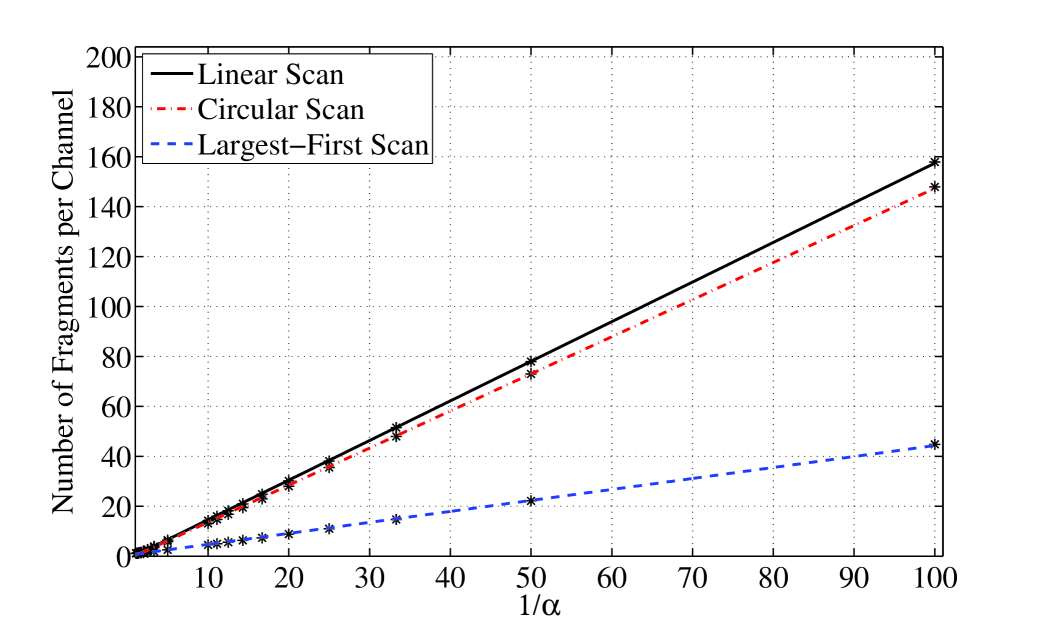
Fig. 7. Average number of fragments per channel.

The average number of fragments per channel is a direct measure of gap-search times, and one that we use here. For values of $\alpha$ expected to be of interest in applications, the effects of CS on gap-search times are only within a few percent relative to LS, as can be seen in Figure 7. The figure also shows the average number of fragments per channel for the Largest-First Scan (LFS) algorithm. This algorithm is designed to speed up the process of finding a set of gaps sufficient to create a new channel. It selects available gaps in a decreasing order of their sizes and allocates them to a request, thereby greedily minimizing the number of gaps needed to fulfill a request. The extra mechanism needed for such a search will of course tend to reduce overall performance gains. The results in Figure 7 for LFS show a surprisingly large improvement in the average number of fragments per channel – as can be seen, a reduction by a factor more than 3 is achieved by LFS for even moderately small $\alpha$.

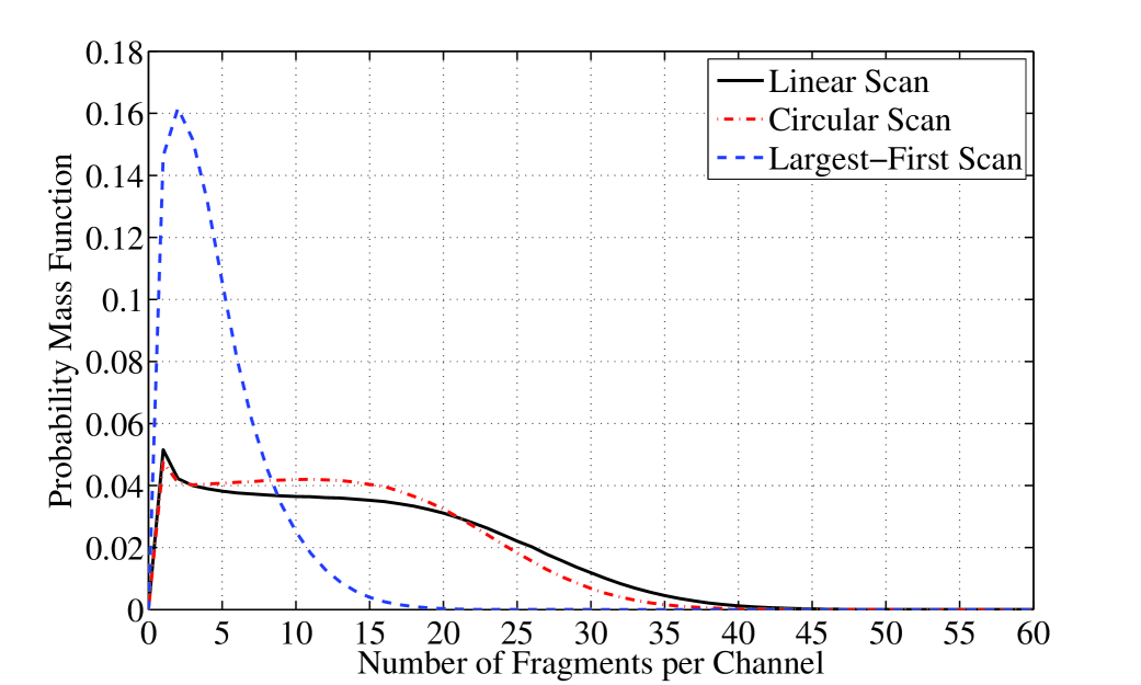
Fig. 8. Distribution of the number of fragments per channel for $\alpha=0.1$.

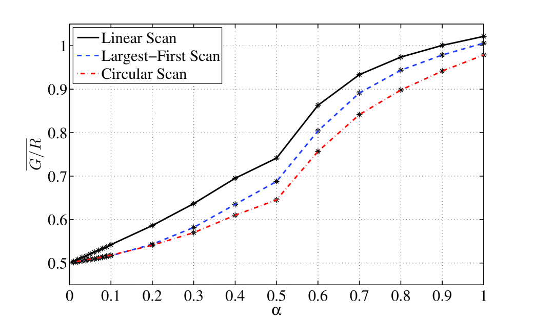
Fig. 9. $\overline{G/R}\rightarrow 1/2$ as $\alpha\rightarrow 0$ under LS, LFS, and CS.

The Probability Mass Functions (pmf’s) of the number of fragments per channel are shown in Figure 8. Notice that while all probabilities are small under LS and CS, the largest applies to the case of no fragmentation at all. The much more peaked distribution for LFS has both much smaller mean and variance: The standard deviation under CS and LS is approximately $1.5$ to $2.0$ times that under LFS. The same limiting behavior called for by the 50% law holds for CS and LFS, which was to be expected, as the arguments supporting the 50% law did not depend on the sequence in which gaps were scanned. But an interesting result of our experiments with CS is that the 50% approximation to expectation of the ratios is within a couple of percent even when the maximum request size is as much as 0.2 the spectrum size. This is easily seen in Figure 9. The convergence rate of LFS to 50% is intermediate between LS and CS.

7. Normal Approximations

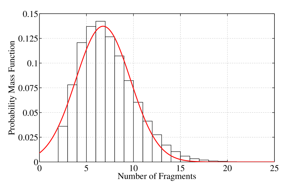
(a) $\alpha=0.5$

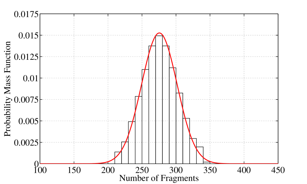
(b) $\alpha=0.1$

Fig. 10. Distributions of the total number of fragments and corresponding Normal fits.

After the usual scaling (i.e., first centering then normalizing by the standard deviation), the scaled version of the number of channels, $R$, tends in probability to the standard Normal, ${\mathcal{N}}(0,1),$ as $M\rightarrow\infty$, where $M=\lfloor 1/\alpha\rfloor$ (it is convenient to express the asymptotics in this section in terms of $M$). This result follows easily from the corresponding heavy-traffic limits in [5, 6], and the ergodicity of $(R(t))$.

Interestingly, it was discovered in the experiments that a normal limit law also appears to hold for the total number $F$ of fragments as $M\rightarrow\infty$ (see for example Figure 10). This is not surprising, since $F$ is the sum over all requests in system of the numbers $F_{i},~{}1\leq i\leq R,$ of fragments allocated to requests. The requests have a mutual dependence, but one whose effect can be expected to weaken for large $M$. As illustrated in Figure 7, the mean of $F_{i}$ is proportional to $M$. Our experiment indicate that the standard deviation of $F_{i}$ is also approximately proportional to $M$. Hence, if $\stackrel{{\scriptstyle p}}{{\rightarrow}}$ denotes convergence in probability as $M\rightarrow\infty$, then

(14) $${F-\beta M^{2}\over\theta M^{3/2}}\stackrel{{\scriptstyle p}}{{\rightarrow}}{\mathcal{N}}(0,1)$$

with $\beta\approx 1.5$ and $\theta\approx 0.9$ formalizes the normal-limit law suggested by our experiments.

Note the two departures from the standard Central Limit Theorem set-up. First, consistent with the linear fragmentation observation, individual request fragmentation scales linearly in $M$, so that the total number of fragments scales as $M^{2}$. Restating the limit law in terms of the sums of random variables ($F_{i}/M$) clearly eliminates this discrepancy. Second, the number of channels ($R$) is random and satisfies the normal limit law discussed above. Thus, the plausibility of (14) requires an appeal to Central Limit Theorems for random sums (e.g., see [14], p. 258, for an appropriate version). Finally, Figure 10 gives some idea of the convergence of the fits to the normal density; as can be seen, fits for $\alpha\leq 0.1$ are indeed close to the simulation data.

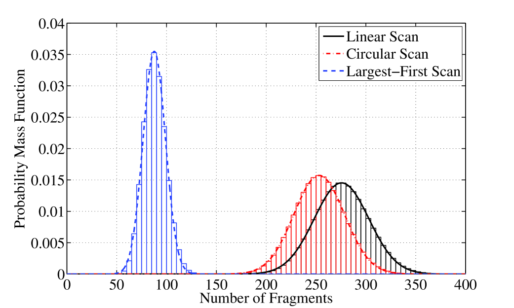
Fig. 11. Distributions of the total number of fragments for $\alpha=0.1$ and the corresponding Normal fits.

We note that the normal approximations shown for the total number of fragments under LS were also found to hold under CS and LFS. This is illustrated in Figure  11.

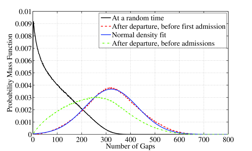
Fig. 12. Distributions of the number of gaps at different epochs for $\alpha=0.01$.

The distributions of the number of gaps at different epochs are shown in Figure 12. The distribution at a random time shows a decreasing pmf. What appeared to be yet another normal approximation was discovered when looking at the first-admission pmf in Figure 12; this is the distribution as seen by the first admission immediately after a departure at just those epochs when there is at least one admission. The third curve is the pmf of the number, $G^{-},$ of gaps as seen right after departures, but before determining whether or not the head of the queue fits in the total available bandwidth. The fit to the Normal density is also illustrated in the figure. The proof of a similar limit law for Renyi’s space-filling problem can be found in [9], but extension of known techniques once again faces the difficult challenges posed by our more difficult fragmentation problem.

8. Conclusions

The results of this paper prepare the ground for further research on several fronts. Before listing a number of the more important ones, we review what we have learned. Our experiments brought out first an unexpected reappearance of a 50% rule relating the expected numbers of gaps and channels in the limit of small request sizes relative to the spectrum size. In our case, we were able to prove the limit law. The next result described a linear relationship between the maximum request size, $\alpha$, and the expected number of fragments into which a request was divided at the time of allocation. Interestingly, the smaller $\alpha$ was taken, the greater was the resulting fragmentation of requests.

Our stability results established the beginning of a mathematical foundation of fragmentation processes. Particularly, we showed that for $\alpha>1/2$, the fragmentation process is Harris recurrent. For general $\alpha$, we proved (with considerable effort) that the total number of fragments is bounded in expected value. We examined alternative algorithms for sequencing through the available gaps and showed that using the LFS algorithm leads to significantly less fragmentation than using the LS or CS algorithms. Finally, we exhibited experimentally a limiting, small-$\alpha$ behavior in which, with appropriate scaling, distributions tend to Normal.

A broad direction for further research extends the parameters of our mathematical model. For instance, while Uniform distributions are generally the assumption of choice in fragmentation models, it would be interesting to see what new effects are created by other distributions of request size, e.g., by varying $a$ in the generalized uniform distributions on $[0,\alpha]$, with densities $x^{a}/\alpha^{a+1}.$ The exponential residence-time assumption is likely to yield simplifications to analysis, but changes in behavior resulting from other distributions are worth investigating. Moreover, instead of a system operating at capacity, in which there is always a request waiting, one could adopt an underlying, fully stochastic model of demand, e.g., a Poisson arrival process, as found in [22].

More realistic, but in all likelihood significantly more difficult models, would relax the independence assumptions. A prime example appropriate for Dynamic Spectrum Access applications would be allowing residence times to depend on fragmentation, the greater the fragmentation of a request, the longer its residence time.

The results regarding the performance of the different algorithms imply that the algorithms’ design should also be considered carefully. Some examples of algorithms that come to mind will aim to better fit the fragments into the available gaps. A more challenging objective would be to develop algorithms that take into account spectrum sensing capabilities during the gap allocation process.

Finally, another broad and very important avenue of research that introduces more realistic models discretizes request sizes and the bandwidth allocation process (as is being done while allocating OFDM subcarriers). As in other models of fragmentation, the continuous limit represented in this paper may conceal important effects, or, conversely, it may introduce effects not present in discrete models. We are actively pursuing this avenue of research.

9. Acknowledgments

We would like to thank Charles Bordenave for helpful discussions in relation with Theorem 4. This work was partially supported by NSF grant CNS-0916263 and CIAN NSF ERC under grant EEC-0812072.

Appendix A Tool validation

In the first test of the simulation tool, we allowed arrivals, discretized the spectrum size, and fixed the requested bandwidth, in such a way that the system reduced to a conventional $M/M/k$ queue. We then matched simulation results with those obtained from classical formulas. In all cases checked, the error compared to the exact results was negligible.

Keeping with our continuous model operating at capacity with random bandwidth requests, one finds that there are very few explicit results for measures of interest, even for the process $R(t)$ for the number of channels in the system. Those that do exist can be found in [22] along with the elegant formula below, which unfortunately requires calculations that are rarely tractable.

Theorem 5 (Kipnis and Robert [22]).

Let $S_{n}$ denote the sum of $n$ i.i.d. request sizes. Then, the maximum throughput (expected number of requests in the system) is

$${\mathbb{E}}(R)={\frac{1}{\sum_{n=1}^{+\infty}(1/n)\mathbb{P}(S_{n}\leq 1<S_{n+1})}}={\frac{1}{\sum_{n=2}^{+\infty}(1/n(n-1))\mathbb{P}(S_{n}>1)}}$$

A system with requests that are uniformly distributed on $[0,1]$ is one case that admits of a simple formula. Here, the density of $S_{n}$ on $[0,1]$ is $z^{n-1}/(n-1)!$, and so an easy calculation gives

$${\mathbb{E}}(R)=\frac{1}{e-2}=1.392\ldots$$

Transform methods are used in [22] to evaluate ${\mathbb{E}}(R)$ for other values of $\alpha$. In particular, computations are based on the (numerical) inversion of a Fourier-Laplace transform. To evaluate the accuracy of our simulator, we checked our experimental results against the computations for the values of $\alpha$ shown in Table 1. As can be seen, the numerics agree well with simulations.

Table 1. Averages $\overline{R}$, computed from our experiments, vs. the corresponding values ${\mathbb{E}}(R)$, obtained from the numerical computations in [22], for various values of $\alpha$. Except for the case $\alpha=1$, the latter results were given to two decimal digits only.

$\alpha$	${\mathbb{E}}(R)$	$\overline{R}$		$\alpha$	${\mathbb{E}}(R)$	$\overline{R}$
0.05	39.51	39.325		0.55	2.9	2.892
0.1	19.4	19.317		0.6	2.54	2.541
0.15	12.69	12.653		0.65	2.26	2.261
0.2	9.34	9.306		0.7	2.04	2.039
0.25	7.32	7.303		0.75	1.87	1.868
0.3	5.98	5.961		0.8	1.73	1.731
0.35	5.01	5.003		0.85	1.62	1.621
0.4	4.28	4.275		0.9	1.53	1.531
0.45	3.71	3.709		0.95	1.45	1.456
0.5	3.29	3.281		1	1.392	1.392

Appendix B Proof of Theorem 4

For any $0<\varepsilon\leq\lambda$,

(15) $$\mathbb{E}_{y}\left(e^{\varepsilon f(Y_{n+1})}\right)=\mathbb{E}_{y}\left(\mathbb{E}_{Y_{n}}\left(e^{\varepsilon(f(Y_{1})-f(Y_{0}))}\right)e^{\varepsilon f(Y_{n})}\mathbbm{1}_{\{f(Y_{n})\leq K\}}\right)\\ +\mathbb{E}_{y}\left(\mathbb{E}_{Y_{n}}\left(e^{\varepsilon(f(Y_{1})-f(Y_{0}))}\right)e^{\varepsilon f(Y_{n})}\mathbbm{1}_{\{f(Y_{n})>K\}}\right).$$

Since by assumption, $f(Y_{1})-f(Y_{0})$ under $\mathbb{P}_{y}$ is stochastically dominated by $Z$ for every $y$, one gets

$$\mathbb{E}_{Y_{n}}\left(e^{\varepsilon(f(Y_{1})-f(Y_{0}))}\right)\leq\mathbb{E}\left(e^{\varepsilon Z}\right)=\mathbb{E}\left(e^{\lambda Z}\right)\stackrel{{\scriptstyle\text{def.}}}{{=}}D$$

and therefore

(16) $$\mathbb{E}_{y}\left(\mathbb{E}_{Y_{n}}\left(e^{\varepsilon(f(Y_{1})-f(Y_{0}))}\right)e^{\varepsilon f(Y_{n})}\mathbbm{1}_{\{f(Y_{n})\leq K\}}\right)\leq De^{\varepsilon K}.$$

For the second term, we apply Lemma 4 to the random variable $f(Y_{1})-f(Y_{0})$ under $\mathbb{P}_{Y_{n}}$:

$$\mathbb{E}_{Y_{n}}\left(e^{\varepsilon(f(Y_{1})-f(Y_{0}))}\right)\leq 1+\varepsilon\mathbb{E}_{Y_{n}}(f(Y_{1})-f(Y_{0}))+c\varepsilon^{2}.$$

Thus, on the event $\{f(Y_{n})>K\}$, one gets

(17) $$\mathbb{E}_{Y_{n}}\left(e^{\varepsilon(f(Y_{1})-f(Y_{0}))}\right)\leq 1-\gamma\varepsilon+c\varepsilon^{2}\stackrel{{\scriptstyle\text{def}}}{{=}}\rho_{\varepsilon}$$

and finally

(18) $$\mathbb{E}_{y}\left(\mathbb{E}_{Y_{n}}\left(e^{\varepsilon(f(Y_{1})-f(Y_{0}))}\right)e^{\varepsilon f(Y_{n})}\mathbbm{1}_{\{f(Y_{n})>K\}}\right)\leq\rho_{\varepsilon}\mathbb{E}_{y}\left(e^{\varepsilon f(Y_{n})}\right).$$

Gathering the two bounds (16) and (18) in (15) finally gives

$$\mathbb{E}_{y}\left(e^{\varepsilon f(Y_{n+1})}\right)\leq\rho_{\varepsilon}\mathbb{E}_{y}\left(e^{\varepsilon f(Y_{n})}\right)+De^{\varepsilon K}$$

which leads by induction to

$$\mathbb{E}_{y}\left(e^{\varepsilon f(Y_{n})}\right)\leq\rho_{\varepsilon}^{n}e^{\varepsilon f(y)}+\frac{1-\rho_{\varepsilon}^{n+1}}{1-\rho_{\varepsilon}}De^{\varepsilon K}.$$

Let $\eta=\big{(}\varepsilon/(2\gamma)\big{)}\wedge\lambda$. From the definition of $\rho_{\varepsilon}$ in  (17), one can easily check that $0<\rho_{\eta}<1$. Therefore, choosing $\varepsilon=\eta$ gives the result.

References

- [1] I. F. Akyildiz, W.-Y. Lee, and K. R. Chowdhury. CRAHNs: Cognitive radio ad hoc networks. Ad Hoc Networks, 7(5):810–836, 2009.
- [2] I. F. Akyildiz, W.-Y. Lee, M. C. Vuran, and S. Mohanty. NeXt generation/dynamic spectrum access/cognitive radio wireless networks: A survey. Comput. Netw., 50(13):2127–2159, Sep. 2006.
- [3] S. Asmussen. Applied Probability and Queues. Springer, New York, NY, USA, 2nd edition, 1987.
- [4] V. G. Bose, A. B. Shah, and M. Ismert. Software radios for wireless networking. In Proc. IEEE INFOCOM’98, Apr. 1998.
- [5] E. G. Coffman, Jr., A. A. Puhalskii, and M. I. Reiman. Storage limited queues in heavy traffic. Probab. Eng. and Info. Sci., 5(4):499–522, 1991.
- [6] E. G. Coffman, Jr. and M. I. Reiman. Diffusion approximations for storage processes in computer systems. In Proc. ACM SIGMETRICS’83, 1983.
- [7] DARPA XG WG, BBN Technologies. The XG architectural framework version 1.0. 2003.
- [8] DARPA XG WG, BBN Technologies. The XG vision RFC version 2.0. 2003.
- [9] A. Dvoretsky and H. Robbins. On the ‘parking’ problem. Publ. Math. Inst. Hung. Acad. Sci., 9:209–226, 1964.
- [10] European Telecommunications Standards Institute. ETSI Reconfigurable Radio. Documentation available at http://www.etsi.org/WebSite/technologies/RRS.aspx.
- [11] FCC. 03-222, Notice of Proposed Rulemaking, Oct. 2003.
- [12] FCC. 05-57, Report and Order, ET Docket No. 03-108, Facilitating Opportunities for Flexible, Efficient, and Reliable Spectrum Use Employing Cognitive Radio Technologies, Mar. 2005.
- [13] FCC. 08-260, Second Report and Order, ET Docket No. 04-186, Unlicensed Operation in the TV Broadcast Bands, Nov. 2008.
- [14] W. Feller. An Introduction to Probability Theory and Its Applications, Volume II. John Wiley & Sons, New York, NY, USA, 2nd edition, 1966.
- [15] S. Geirhofer, L. Tong, and B. Sadler. Interference-aware OFDMA resource allocation: A predictive approach. In Proc. IEEE MILCOM’08, Nov. 2008.
- [16] A. Ghasemi and E. Sousa. Spectrum sensing in cognitive radio networks: Requirements, challenges and design trade-offs. IEEE Commun., 46(4):32–39, Apr. 2008.
- [17] B. Hajek. Hitting-time and occupation-time bounds implied by drift analysis with applications. Adv. Appl. Probab., 14(3):502–525, 1982.
- [18] W. Hou, L. Yang, L. Zhang, X. Shan, and H. Zheng. Understanding cross-band interference in unsynchronized spectrum access. In Proc. ACM CoRoNet’09, 2009.
- [19] IEEE 802.22, Working Group on Wireless Regional Area Networks (“WRANs”). Documentation available at http://ieee802.org/22/.
- [20] IEEE Standards Coordinating Committee 41 (Dynamic Spectrum Access Networks). Documentation available at http://www.scc41.org/.
- [21] J. Jia, Q. Zhang, and X. Shen. HC-MAC: A hardware-constrained cognitive MAC for efficient spectrum management. IEEE J. Sel. Areas Commun., 26(1):106–117, Jan. 2008.
- [22] C. Kipnis and P. Robert. A dynamic storage process. Stochastic processes and their applications, 34(1):155–169, 1990.
- [23] D. E. Knuth. The Art of Computer Programming, Vol. 1 - Fundamental Algorithms. Addison Wesley Longman Publishing Co., Redwood City, CA, USA, 3rd edition, 1997.
- [24] W. Krenik, A. M. Wyglinski, and L. E. Doyle (eds.). Cognitive radios for dynamic speactrm access. Special Issue, IEEE Commun., 45(5):64–65, May 2007.
- [25] H. Mahmoud, T. Yucek, and H. Arslan. OFDM for cognitive radio: Merits and challenges. IEEE Wireless Commun., 16(2):6–15, Apr. 2009.
- [26] P. Mahonen and M. Zorzi (eds.). Cognitive wireless networks. Special Issue, IEEE Wireless Commun., 14(4):4–5, Aug. 2007.
- [27] J. Mitola III. Cognitive radio for flexible mobile multimedia communications. In Proc. IEEE MoMuC’99, Nov. 1999.
- [28] J. Mitola III. Cognitive Radio: An Integrated Agent Architecture for Software Defined Radio. PhD thesis, Doctor of Technology, Royal Inst. Technol. (KTH), Stockholm, Sweden, 2000.
- [29] J. D. Poston and W. D. Horne. Discontiguous OFDM considerations for dynamic spectrum access in idle TV channels. In Proc. IEEE DySPAN’05, Nov. 2005.
- [30] R. Rajbanshi, A. M. Wyglinski, and G. J. Minden. OFDM-based cognitive radios for dynamic spectrum access networks. In V. K. Bhargava and E. Hossain, editors, Cognitive Wireless Communication Networks, pages 165–188. Springer-Verlag, 2007.
- [31] A. Shukla, B. Willamson, J. Burns, E. Burbidge, A. Taylor, and D. Robinson. A study for the provision of aggregation of frequency to provide wider bandwidth services. Technical report, QinetiQ, Aug. 2006.
- [32] T. A. Weiss and F. K. Jondral. Spectrum pooling: An innovative strategy for the enhancement of spectrum efficiency. IEEE Commun., 42(3):S8–14, Mar. 2004.
- [33] Y. Yuan, P. Bahl, R. Chandra, T. Moscibroda, and Y. Wu. Allocating dynamic time-spectrum blocks in cognitive radio networks. In Proc. ACM MobiHoc’07, 2007.