Abstract

In this paper we study the relation between long cycles and Bose-Einstein condensation in the Infinite-Range Bose-Hubbard Model. We obtain an expression for the cycle density involving the partition function for a Bose-Hubbard Hamiltonian with a single-site correction. Inspired by the Approximating Hamiltonian method we conjecture a simplified expression for the short cycle density as a ratio of single-site partition functions. In the absence of condensation we prove that this simplification is exact and use it to show that in this case the long-cycle density vanishes. In the presence of condensation we can justify this simplification when a gauge-symmetry breaking term is introduced in the Hamiltonian. Assuming our conjecture is correct, we compare numerically the long-cycle density with the condensate and find that though they coexist, in general they are not equal.

Keywords: Bose-Einstein Condensation, Cycles, Infinite-Range Bose-Hubbard Model
PACS: 03.75.Hh, 67.25.de, 67.85.Bc.

1 Introduction

Motivated by the path-integral formulation, in 1953 Feynman [1] studied the relation between the statistical distribution of particles on permutation cycles and the occurrence of Bose-Einstein condensation (BEC). He conjectured that the presence of long cycles is intrinsically connected to BEC. Penrose and Onsager developed these arguments and observed that BEC should occur when the fraction of the total number of particles belonging to long cycles is strictly positive [2]. These concepts, which are now generally accepted, were made mathematically precise by Sütő [3] who also proved the equivalence between the Bose-condensate density and the density of the number of particles on long cycles in the case of the free and mean-field Bose gas (see also Ueltschi [4]). Subsequently it was shown that this relation holds for the perturbed mean-field model of a Bose gas [5]. In our previous paper the validity of this hypothesis was tested in another model of a Bose gas, the Infinite-Range-Hopping Bose-Hubbard Model with Hard Cores [6]. There it was shown that while the existence of non-zero long cycle density and BEC coincide, these densities were not necessarily equal.

This paper is the sequel to [6], where now the hard-core interaction is replaced with a finite on-site repulsion to discourage but not forbid multiple particle occupation of individual sites. The thermodynamics of this model have been studied by Bru and Dorlas [7]. They show that the phase diagram for this model is much more complicated than in the hard-core case as for low enough temperatures there are several critical values of chemical potential which correspond to intervals of BEC (see Fig 2). As in [6], we use standard properties of the decomposition of permutations into cycles, to convert the grand-canonical sum into a sum on cycle lengths. This makes it possible to decompose the total density $\rho=\rho_{\rm short}+\rho_{\rm long}$ into the density of particles belonging to cycles of finite length ($\rho_{\rm short}$) and to infinitely long cycles ($\rho_{\rm long}$) in the thermodynamic limit. We consider the relationship between Bose-condensation and long cycles in this model.

The model is considered in the grand-canonical ensemble. In terms of the random walk representation, the particles hop from one site to another with probability depending on the occupation number of the destination site – the more particles on the site, the less likely another particle will hop there. Following [6] we write the cycle density for the number of particles on a cycle of length $q$ in terms of a partition function of $q$ distinguishable particles interacting with the Boson system. Again as in [6] we exploit the fact that the hopping between the $q$ distinguishable particles can be neglected, to obtain an expression for the cycle density in terms of the ratio of the partition function for a Bose-Hubbard Hamiltonian with a single-site correction and it without. Inspired by the Approximating Hamiltonian method [8] we conjecture a simplified expression for the short cycle density $\rho_{\rm short}$ as a ratio of single-site partition functions. We prove that this simplification is exact in the absence of condensation and implies a zero long-cycle density in this case. Unfortunately we are not able to prove this simplifying conjecture when BEC occurs, however we can go some way towards justifying it by introducing a gauge-symmetry breaking term in the Hamiltonians. Assuming our conjecture is correct, we perform some simple numerical techniques to compare the long-cycle density with the condensate. We find (as in [6]) that though they coexist, in general they are not equal.

Before describing the layout of this paper, it is worth noting that BEC may be classified into three types (see [9] and [10]): type I/II when a finite/infinite number of one-particle quantum states are macroscopically occupied (resp.), and type III when no states are macroscopically occupied. The relation between the size of long cycles and these condensate types for the free Bose gas is considered in [11].

The paper is structured as follows. In Section 2 we first describe the model and recall its thermodynamic properties as stated by Bru and Dorlas [7]. In Section 3, by applying the general framework for cycle statistics described in [5] (following [12]), we form an expression for the density of cycles of length $q$ by isolating $q$ distinguishable particles from the boson field and show that we can neglect the hopping of these $q$ particles in the thermodynamic limit. Section 4 deals with the above conjecture, proving its correctness in the absence of condensation and proving an equivalent result with the addition of a gauge-symmetry breaking term to the Hamiltonian which is correct in the absence and presence of BEC. Section 5 proves that in the absence of BEC the long cycle density is zero.

2 The Model and Results

The Bose-Hubbard Hamiltonian is given by

$$H^{\mathrm{BH}}_{\hbox{\tiny{$V$}}}=J\!\!\!\!\!\!\sum_{x,y\in\Lambda_{\hbox{\tiny{$V$}}}\,:|x-y|=1}(a^{\ast}_{x}-a^{\ast}_{y})(a^{\phantom{*}}_{x}-a^{\phantom{*}}_{y})+\lambda\sum_{x\in\Lambda_{{\hbox{\tiny{$V$}}}}}n_{x}(n_{x}-1)$$ (2.1)

where $\Lambda_{\hbox{\tiny{$V$}}}$ is a lattice of $V$ sites, $a^{\ast}_{x}$ and $a^{\phantom{*}}_{x}$ are the Bose creation and annihilation operators satisfying the usual commutation relations $[a^{\ast}_{x},a^{\phantom{*}}_{y}]=\delta_{x,y}$ and $n_{x}=a^{\ast}_{x}a^{\phantom{\ast}}_{x}$. The first term with $J>0$ is the kinetic energy operator and the second term with $\lambda>0$ describes a repulsive interaction, as it discourages the presence of more than one particle at each site. This model was originally introduced by Fisher et al. [13].

The infinite-range hopping model is given by the Hamiltonian

$$H_{\hbox{\tiny{$V$}}}=\frac{1}{2V}\!\!\!\sum_{x,y\in\Lambda_{\hbox{\tiny{$V$}}}}(a^{\ast}_{x}-a^{\ast}_{y})(a^{\phantom{*}}_{x}-a^{\phantom{*}}_{y})+\lambda\sum_{x\in\Lambda_{\hbox{\tiny{$V$}}}}n_{x}(n_{x}-1).$$ (2.2)

This is in fact a mean-field version of (2.1) but in terms of the kinetic energy rather than the interaction. In particular, as with all mean-field models, the lattice structure is irrelevant and there is no dependence on dimensionality, so we can take $\Lambda_{\hbox{\tiny{$V$}}}=\{1,2,3,\ldots,V\}$. The non-zero temperature properties of this model have been studied by Bru and Dorlas [7] and by Adams and Dorlas [14]. Also Dorlas, Pastur and Zagrebnov [15] considered the model in the presence of an additional random potential.

Bru and Dorlas applied the “Approximating Hamiltonian” method (see [8, 16]) to the Infinite-Range-Hopping Bose-Hubbard Model. In this method one performs the following substitution for the Laplacian term of the Hamiltonian:

$$\frac{1}{V}\sum_{x,y=1}^{V}a^{\ast}_{x}a^{\phantom{*}}_{y}\rightarrow\sum_{x=1}^{V}(\bar{r}a^{\phantom{*}}_{x}+ra^{\ast}_{x})-V|r|^{2}$$

(some $r\in\mathbb{C}$) to obtain the approximating Hamiltonian:

$$H^{\textrm{APP}}_{\hbox{\tiny{$V$}}}(r)=\sum_{x=1}^{V}n_{x}-\sum_{x=1}^{V}(\bar{r}a^{\phantom{*}}_{x}+ra^{\ast}_{x})+V|r|^{2}+\lambda\sum_{x=1}^{V}n_{x}(n_{x}-1).$$ (2.3)

Introduce a gauge breaking source $\nu\in\mathbb{C}$ in both Hamiltonians (2.2) and (2.3), by setting $H_{\hbox{\tiny{$V$}}}(\nu)\vcentcolon=H_{\hbox{\tiny{$V$}}}-\sum_{x=1}^{V}(\bar{\nu}a^{\phantom{*}}_{x}+\nu a^{\ast}_{x})$ and $H^{\textrm{APP}}_{\hbox{\tiny{$V$}}}(r,\nu)\vcentcolon=H^{\text{APP}}_{\hbox{\tiny{$V$}}}(r)-\sum_{x=1}^{V}(\bar{\nu}a^{\phantom{*}}_{x}+\nu a^{\ast}_{x})$. Then for all $\mu$ and $\nu$, one finds that the pressures for these Hamiltonians are equivalent in the thermodynamic limit, i.e. for large $V$ one obtains the estimate

$$0\leq p_{\hbox{\tiny{$V$}}}[H_{\hbox{\tiny{$V$}}}(\nu)]-\sup_{r\in\mathbb{C}}p_{\hbox{\tiny{$V$}}}[H^{\textrm{APP}}_{\hbox{\tiny{$V$}}}(r,\nu)]\leq O(V^{-1/2})$$

where for a Hamiltonian $H$, $p_{\hbox{\tiny{$V$}}}[H]\vcentcolon=p_{\hbox{\tiny{$V$}}}[H](\beta,\mu)$ denotes the corresponding grand-canonical pressure. Henceforth the $\beta$ and $\mu$ dependencies are assumed unless explicitly given.

With this technique, Bru and Dorlas managed to obtain the limiting pressure and showed that in some regimes Bose-Einstein condensation occurs. They proved the following result:

Theorem 2.1

The pressure in the thermodynamic limit for the Infinite-Range-Hopping Bose-Hubbard Model, $p(\beta,\mu)\vcentcolon=\lim_{V\to\infty}p_{\hbox{\tiny{$V$}}}[H_{\hbox{\tiny{$V$}}}]$, is given by

$$p(\beta,\mu)=\sup_{r\geq 0}\bigg{\{}-r^{2}+\frac{1}{\beta}\ln\text{\rm{trace}}\,_{\mathcal{F}_{+}(\mathbb{C})}\mathrm{e}^{-\beta h(r)}\bigg{\}}$$ (2.4)

where

$$h(r)\vcentcolon=(1-\mu)n+\lambda n(n-1)-r(a+a^{\ast})$$

is a single site Hamiltonian with creation and annihilation operators $a^{\ast}$ and $a$, and with number operator $n=a^{\ast}a$. Note that it is sufficient to take the supremum over the set of non-negative real numbers.

The Euler-Lagrange equation for the variational principle is

$$2r=\big{\langle}a+a^{\ast}\big{\rangle}_{h(r)}\vcentcolon=\frac{\text{\rm{trace}}\,_{\mathcal{F}(\mathbb{C})}(a+a^{\ast})\mathrm{e}^{-\beta h(r)}}{\text{\rm{trace}}\,_{\mathcal{F}(\mathbb{C})}\mathrm{e}^{-\beta h(r)}}.$$ (2.5)

Moreover the density of the condensate is exactly given by

$${\rho^{\mu}_{{\rm c\phantom{l}}}}\vcentcolon=\lim_{V\to\infty}\frac{1}{V^{2}}\sum_{x,y=1}^{V}\big{\langle}a^{\ast}_{x}a^{\phantom{*}}_{y}\big{\rangle}_{H_{\hbox{\tiny{$V$}}}}=r_{\mu}^{2}.$$

where $r_{\mu}$ is the largest solution of $(\ref{euler-lagrange})$.

Equation (2.5) can have at most two solutions. Clearly $r=0$ is always a solution. When $\beta$ is large enough, for certain values of $\mu$ a second non-zero solution may appear (see Fig 1). So $r_{\mu}\vcentcolon=0$ unless a second solution $r>0$ exists, in which case $r_{\mu}\vcentcolon=r$.

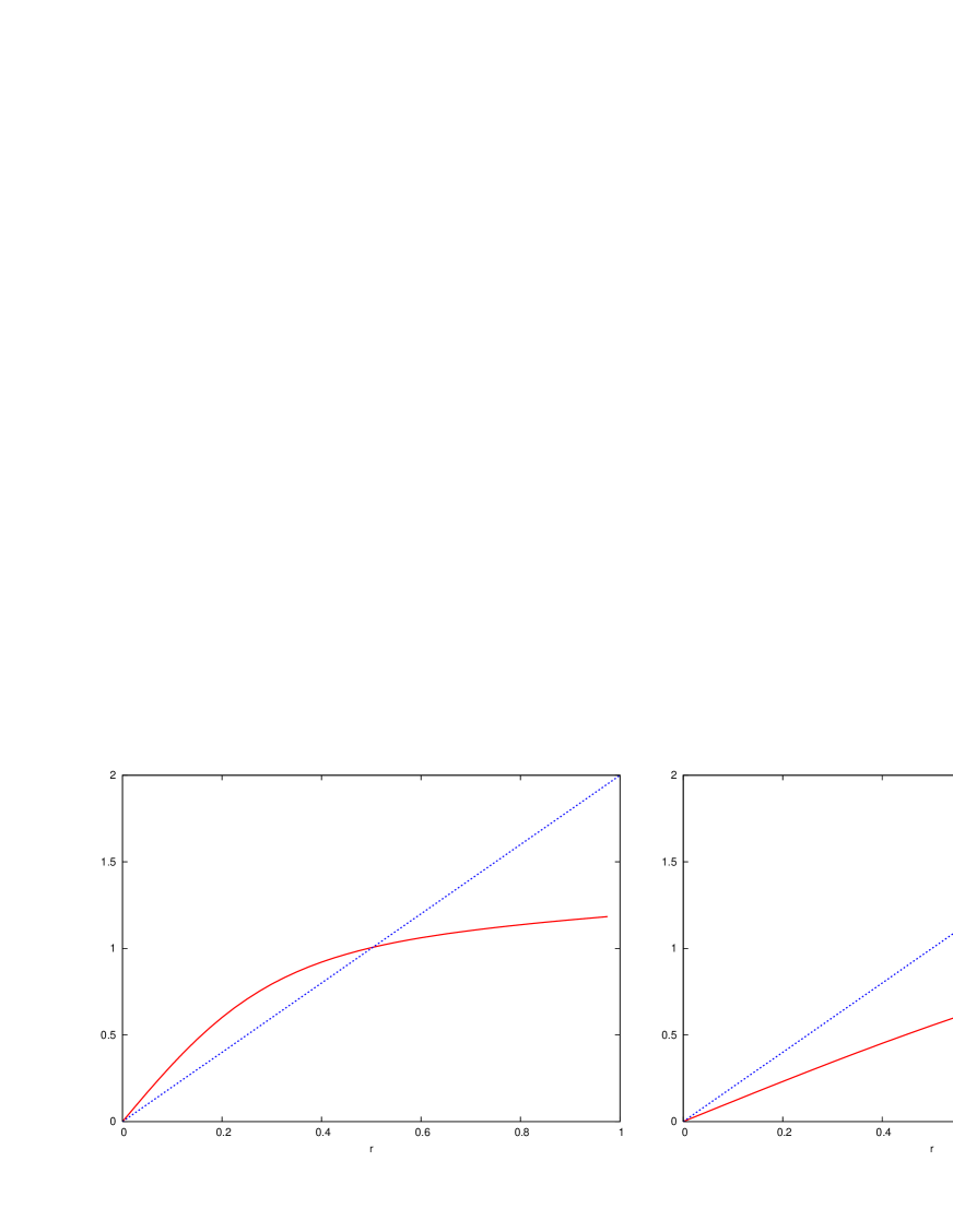
Figure 1: Comparison of $2r$ with $\langle a+a^{\ast}\rangle_{h(r)}$ with $\beta=4$, $\lambda=5$ for the cases $\mu=1.5$ (condensation) and $\mu=5$ (no condensation).

The properties of this model were then obtained numerically by finding this maximal solution of the Euler-Lagrange equation and then evaluating the pressure using (2.4). As may be seen from Fig 2, for sufficiently large $\beta$, there may exist several critical values of $\mu$ which correspond to intervals of $r_{\mu}=0$ and $r_{\mu}>0$.

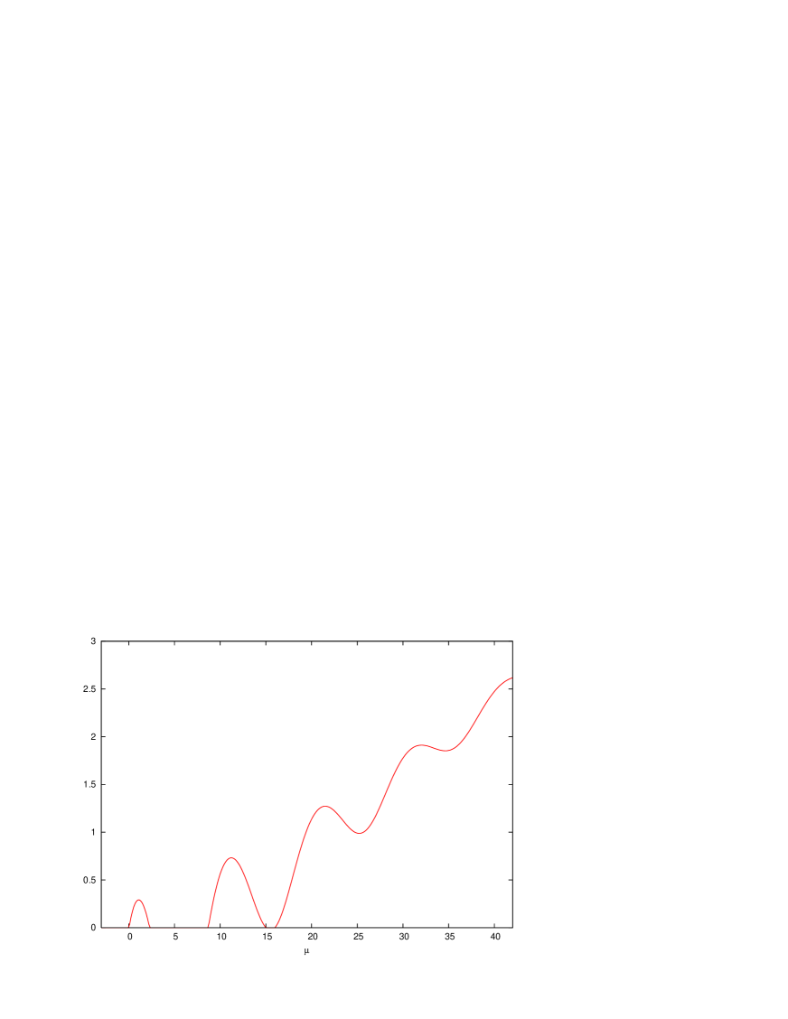
Figure 2: Plot of the condensate density $r_{\mu}^{2}(={\rho^{\mu}_{{\rm c\phantom{l}}}})$ versus $\mu$, for $\beta=4$, $\lambda=5$.

In addition Bru and Dorlas showed that Theorem 2.1 holds in the presence of the gauge-symmetry breaking term. In that case, the corresponding Euler-Lagrange equation has a unique non-zero solution $r_{\mu}(\nu)$.

In this paper we shall analyse the cycle statistics of this model. $H_{\hbox{\tiny{$V$}}}$ is a grand-canonical Hamiltonian given by (2.2) acting upon the bosonic Fock space $\mathcal{F}_{+}({\mathcal{H}_{\hbox{\tiny{$V$}}}})$. Let $H_{\hbox{\tiny{$V$}}}^{(n)}$ be the restriction of $H_{\hbox{\tiny{$V$}}}$ to the $n$ particle space ${\mathcal{H}_{{\hbox{\tiny{$V$}}}}^{(n)}}$, and its corresponding symmetrised subspace ${\mathcal{H}_{{\hbox{\tiny{$V$}}},+}^{(n)}}$. Then the grand-canonical partition function for this model may be written as

$$\Xi_{\hbox{\tiny{$V$}}}^{\mu} =\text{\rm{trace}}\,_{\mathcal{F}_{+}({\mathcal{H}_{\hbox{\tiny{$V$}}}})}\left[\mathrm{e}^{-\beta(H_{\hbox{\tiny{$V$}}}-\mu N_{\hbox{\tiny{$V$}}})}\right]=\sum_{n=0}^{\infty}\text{\rm{trace}}\,_{{\mathcal{H}_{{\hbox{\tiny{$V$}}},+}^{(n)}}}\left[\mathrm{e}^{-\beta(H_{\hbox{\tiny{$V$}}}^{(n)}-\mu n)}\right]$$

$$=\sum_{n=0}^{\infty}\frac{1}{n!}\sum_{\pi\in S_{n}}\text{\rm{trace}}\,_{{\mathcal{H}_{{\hbox{\tiny{$V$}}}}^{(n)}}}\left[U_{\pi}\mathrm{e}^{-\beta(H_{\hbox{\tiny{$V$}}}^{(n)}-\mu n)}\right].$$

where $S_{n}$ is the set of all permutations of $n$ items, and $U_{\pi}$ the unitary representation of a permutation $\pi\in S_{n}$.

There is a natural probability measure (see [5]) on the set of all permutations $\bigcup_{n=0}^{\infty}S_{n}$ (taking $S_{0}=\{1\}$) defined as

$$\mathbb{P}^{\mu}_{\hbox{\tiny{$V$}}}(\pi)=\frac{1}{\Xi_{\hbox{\tiny{$V$}}}^{\mu}}\sum_{n=0}^{\infty}\frac{1}{n!}\text{\rm{trace}}\,_{{\mathcal{H}_{{\hbox{\tiny{$V$}}}}^{(n)}}}\left[U_{\pi}e^{-\beta(H_{\hbox{\tiny{$V$}}}^{(n)}-\mu n)}\right]\mathcal{I}_{S_{n}}(\pi)$$

where $\mathcal{I}$ is the indicator function, ensuring $\pi\in S_{n}$ for some $n$.

From the random walk formulation (see for example [17]) one can see that the kernel of $\mathrm{e}^{-\beta H_{\hbox{\tiny{$V$}}}^{(n)}}$ is positive and therefore the righthand side of this expression is positive.

Each permutation $\pi\in S_{n}$ can be decomposed uniquely into a number of cyclic permutations of lengths $q_{1},q_{2},\dots,q_{j}$ with $j\leq n$ and $q_{1}+q_{2}+\dots+q_{j}=n$. For $q\in\{1,2,\ldots,n\}$, let $N_{q}(\pi)$ be the random variable corresponding to the number of cycles of length $q$ in $\pi$. Then the expectation of the number of $q$-cycles in the grand canonical ensemble is

$$\mathbb{E}^{\mu}_{\hbox{\tiny{$V$}}}(N_{q})=\sum_{j=0}^{\infty}j\mathbb{P}^{\mu}_{\hbox{\tiny{$V$}}}(N_{q}\!=\!j)$$

and the average density of particles in $q$-cycles is

$$c^{\mu}_{\hbox{\tiny{$V$}}}(q)=\frac{q\;\mathbb{E}^{\mu}_{\hbox{\tiny{$V$}}}(N_{q})}{V}.$$

This brings us then to the following definition.

Definition 1

The expected density of particles on cycles of finite length is given by

$${\rho^{\mu}_{{\rm short}}}=\lim_{Q\to\infty}\;\lim_{V\to\infty}\;\sum_{q=1}^{Q}c_{\hbox{\tiny{$V$}}}^{\mu}(q)$$ (2.6)

and the expected density of particles on cycles of infinite length is given by

$${\rho^{\mu}_{{\rm long}}}=\lim_{Q\to\infty}\;\lim_{V\to\infty}\;\sum_{q=Q+1}^{\infty}c_{\hbox{\tiny{$V$}}}^{\mu}(q).$$ (2.7)

Clearly ${\rho^{\mu}_{{\phantom{l}}}}={\rho^{\mu}_{{\rm short}}}+{\rho^{\mu}_{{\rm long}}}$.

For brevity, denote $c^{\mu}_{\phantom{l}}(q)=\lim_{V\to\infty}c^{\mu}_{\hbox{\tiny{$V$}}}(q)$. It is clearly easier to deal with ${\rho^{\mu}_{{\rm short}}}$ since we can take the thermodynamic limit inside the sum over $q$ to get

$${\rho^{\mu}_{{\rm short}}}=\sum_{q=1}^{\infty}\;c^{\mu}_{\phantom{l}}(q).$$

For the free Bose gas, the mean-field and the perturbed mean-field Bose gas, it has been shown that ${\rho^{\mu}_{{\rm long}}}={\rho^{\mu}_{{\rm c\phantom{l}}}}$, the condensate density. However in the case of the Hard-Core Infinite-Range-Hopping Bose-Hubbard model (see [6]), a different conclusion was obtained: that ${\rho^{\mu}_{{\rm long}}}>0$ if and only if ${\rho^{\mu}_{{\rm c\phantom{l}}}}>0$, but that in the presence of condensation these quantities were not necessarily equal. We wish to argue that this is also the case for the chosen model.

We now state our results.

Theorem 2.2

The density of cycles of finite length in the IRH Bose-Hubbard model may be expressed as

$${\rho^{\mu}_{{\rm short}}}=\sum_{q=1}^{\infty}\mathrm{e}^{-\beta(q-\mu)q}\lim_{V\to\infty}\frac{\text{\rm{trace}}\,_{\mathcal{F}_{+}({\mathcal{H}_{\hbox{\tiny{$V$}}}})}\exp\big{\{}-\beta(2\lambda qn_{1}+H_{\hbox{\tiny{$V$}}}-\mu N_{\hbox{\tiny{$V$}}})\big{\}}}{\text{\rm{trace}}\,_{\mathcal{F}_{+}({\mathcal{H}_{\hbox{\tiny{$V$}}}})}\exp\big{\{}-\beta(H_{\hbox{\tiny{$V$}}}-\mu N_{\hbox{\tiny{$V$}}})\big{\}}}.$$

where $n_{1}$ is an operator which counts the number of bosons on the site labelled $1$.

If one were to substitute $H_{\hbox{\tiny{$V$}}}$ for the approximating Hamiltonian $H^{\text{APP}}_{\hbox{\tiny{$V$}}}(r_{\mu})$ (where again $r_{\mu}$ is the maximal solution of the Euler-Lagrange equation (2.5)) into the right hand side of this expression, one would obtain:

$${\rho^{\mu}_{{\rm short}}}=\sum_{q=1}^{\infty}\frac{\text{\rm{trace}}\,_{\mathcal{F}_{+}(\mathbb{C})}\mathrm{e}^{-\beta h_{q}(r_{\mu})}}{\text{\rm{trace}}\,_{\mathcal{F}_{+}(\mathbb{C})}\mathrm{e}^{-\beta h_{0}(r_{\mu})}}.$$ (2.8)

where

$$h_{q}(r)\vcentcolon=(1-\mu)(n+q)+\lambda(n+q)(n+q-1)-r(a+a^{\ast})$$

is another single-site Hamiltonian (note that $h_{0}(r)=h(r)$). This leads to the conjecture that (2.8) gives the correct expression for ${\rho^{\mu}_{{\rm short}}}$.

Moreover the fact that a state corresponding to $H_{\hbox{\tiny{$V$}}}$ in the thermodynamic limit may be shown to be a convex combination of one-site product states of the form

$$\omega(A)=\frac{\text{\rm{trace}}\,_{\mathcal{F}_{+}(\mathbb{C})}\mathrm{e}^{-\beta h_{q}(r_{\mu})}A}{\text{\rm{trace}}\,_{\mathcal{F}_{+}(\mathbb{C})}\mathrm{e}^{-\beta h_{0}(r_{\mu})}}$$

supports this conjecture. We prove the conjecture for those values of $\mu$ such that $r_{\mu}=0$, but unfortunately are unable to do so when $r_{\mu}>0$. However we can prove a slightly weaker result with the addition of a gauge-symmetry breaking term.

Let $c_{\hbox{\tiny{$V$}}}^{\mu}(q,\nu)$ be the density of particles on cycles of length $q$ for the gauge-symmetry broken Hamiltonian $H_{\hbox{\tiny{$V$}}}(\nu)$.

Theorem 2.3

For $\mu$ such that $r_{\mu}=0$, we have

$$c^{\mu}_{\phantom{l}}(q)=\frac{\text{\rm{trace}}\,_{\mathcal{F}_{+}(\mathbb{C})}\mathrm{e}^{-\beta h_{q}(0)}}{\text{\rm{trace}}\,_{\mathcal{F}_{+}(\mathbb{C})}\mathrm{e}^{-\beta h_{0}(0)}}.$$

More generally for any $\mu\in\mathbb{R}$, for a fixed $\nu>0$ there exists a sequence $\nu_{\hbox{\tiny{$V$}}}\to\nu$ as $V\to\infty$, independent of $q$ such that

$$\lim_{V\to\infty}c_{\hbox{\tiny{$V$}}}^{\mu}(q,\nu_{\hbox{\tiny{$V$}}})=\frac{\text{\rm{trace}}\,_{\mathcal{F}_{+}(\mathbb{C})}\mathrm{e}^{-\beta[h_{q}(r_{\mu}(\nu))-\nu(a+a^{\ast})]}}{\text{\rm{trace}}\,_{\mathcal{F}_{+}(\mathbb{C})}\mathrm{e}^{-\beta[h_{0}(r_{\mu}(\nu))-\nu(a+a^{\ast})]}}.$$ (2.9)

Note that this theorem implies (2.8) for $r_{\mu}=0$. This allows us to show that in the absence of condensation all particles are on short cycles.

Theorem 2.4

In the absence of condensation, i.e. for those $\mu$ such that $r_{\mu}=0$, the density of particles on short cycles equals the total density of the system, that is:

$${\rho^{\mu}_{{\rm short}}}={\rho^{\mu}_{{\phantom{l}}}}\quad\Rightarrow\quad{\rho^{\mu}_{{\rm long}}}=0.$$

Moreover considering equation (2.9), if the thermodynamic limit and the limit removing the gauge-breaking source are interchangeable then (2.8) follows for any $r_{\mu}$.

Assuming the conjecture is correct, we apply some simple numerical techniques to (2.8) in order to compare long cycles with the Bose-Einstein condensate. As may be seen from Figures 3 and 4 the calculations certainly agree with Theorem (2.4), i.e. that the absence of condensation implies the lack of long cycles and visa versa. However more importantly they also indicate that while the presence of condensation coincides with the existence of long cycles, their respective densities are not necessarily equal. In fact, one can see that the long cycle density may be greater than or less than the condensate density for differing parameters.

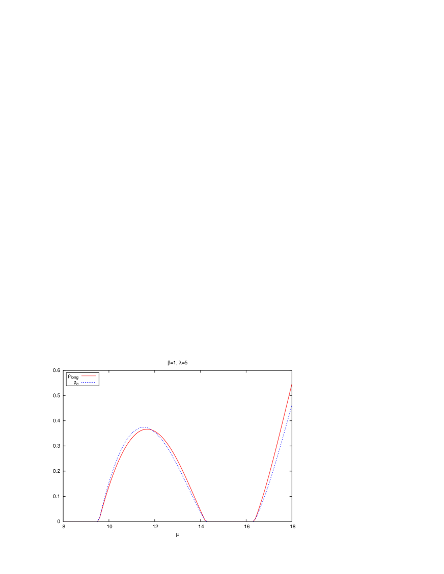
Figure 3: Comparison of ${\rho^{\mu}_{{\rm long}}}$ with ${\rho^{\mu}_{{\rm c\phantom{l}}}}$

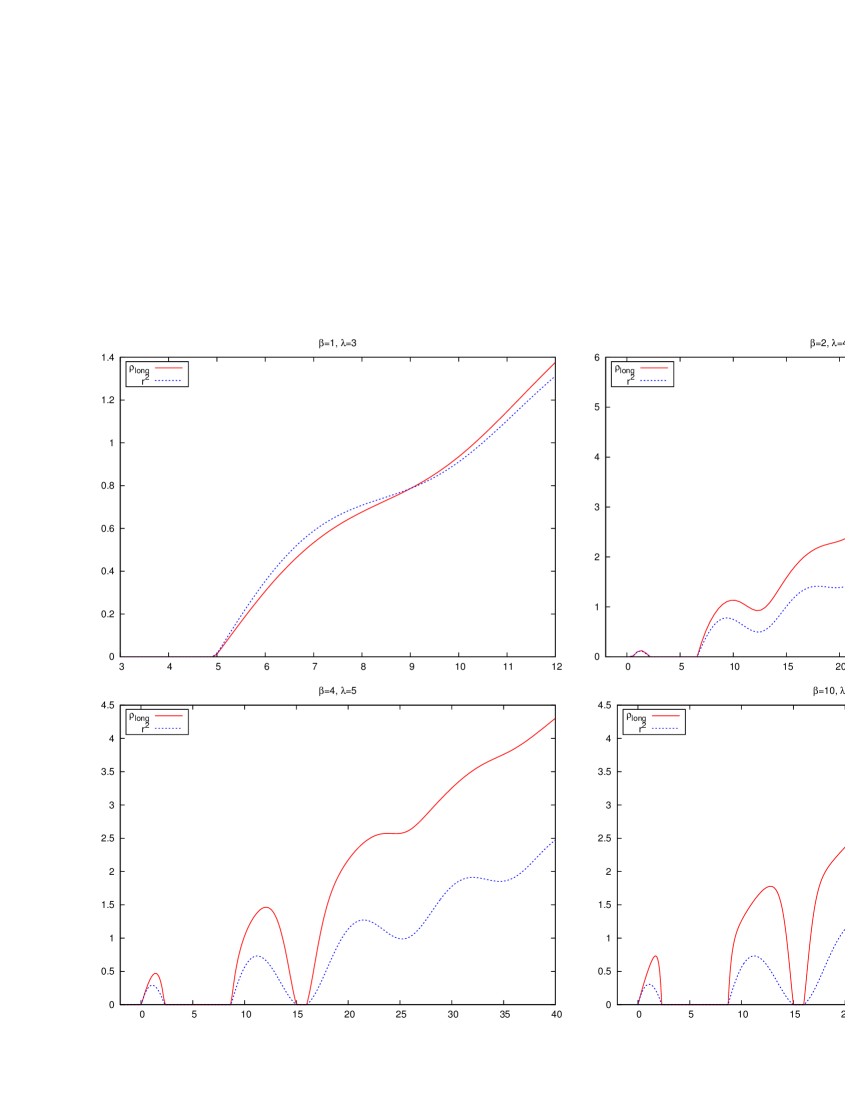
Figure 4: Comparison of ${\rho^{\mu}_{{\rm long}}}$ with ${\rho^{\mu}_{{\rm c\phantom{l}}}}$ for various values of $\beta$ and $\lambda$.

3 Proof of Theorem 2.2

Before proceeding to the study the cycle statistics for this model we need to define the $n$-particle Hamiltonian in more detail. The Hilbert space for a single particle on a lattice of $V$ sites is ${\mathcal{H}_{\hbox{\tiny{$V$}}}}\vcentcolon=\mathbb{C}^{\hbox{\tiny{$V$}}}$ and on it we define the operator

$$h_{\hbox{\tiny{$V$}}}=I-P_{\hbox{\tiny{$V$}}}$$

where $P_{\hbox{\tiny{$V$}}}$ is the orthogonal projection onto the unit vector

$$\mathbf{g}_{\hbox{\tiny{$V$}}}=\frac{1}{\sqrt{V}}\sum_{x=1}^{V}\mathbf{e}_{x}=\frac{1}{\sqrt{V}}(1,1,\dots,1)\in{\mathcal{H}_{\hbox{\tiny{$V$}}}},$$

with $\{\mathbf{e}_{x}\}_{x=1}^{V}$ the usual orthonormal basis for ${\mathcal{H}_{\hbox{\tiny{$V$}}}}$. $h_{\hbox{\tiny{$V$}}}$ is the orthogonal projection onto the subspace orthogonal to $\mathbf{g}_{\hbox{\tiny{$V$}}}$. For an operator $A$ on ${\mathcal{H}_{\hbox{\tiny{$V$}}}}$, we define $A^{(n)}$ on ${\mathcal{H}_{{\hbox{\tiny{$V$}}}}^{(n)}}\vcentcolon=\underbrace{{\mathcal{H}_{\hbox{\tiny{$V$}}}}\otimes{\mathcal{H}_{\hbox{\tiny{$V$}}}}\otimes\dots\otimes{\mathcal{H}_{\hbox{\tiny{$V$}}}}}_{n\text{ times}}$, by

$$A^{(n)}=A\otimes I\otimes\ldots\otimes I+I\otimes A\otimes\ldots\otimes I+\ldots+I\otimes I\otimes\ldots\otimes A.$$

Let $\mathcal{F}({\mathcal{H}_{\hbox{\tiny{$V$}}}})=\bigoplus_{n=0}^{\infty}{\mathcal{H}_{{\hbox{\tiny{$V$}}}}^{(n)}}$ denote the unsymmetrised Fock space of ${\mathcal{H}_{\hbox{\tiny{$V$}}}}$ and define $d\Gamma(A)$ on $\mathcal{F}({\mathcal{H}_{\hbox{\tiny{$V$}}}})$ as

$$d\Gamma(A)=\sum_{n=0}^{\infty}A^{(n)}$$

where ${\mathcal{H}_{\hbox{\tiny{$V$}}}}^{(0)}\vcentcolon=\mathbb{C}$ and ${\mathcal{H}_{\hbox{\tiny{$V$}}}}^{(1)}\vcentcolon={\mathcal{H}_{\hbox{\tiny{$V$}}}}$. With this notation we can write the free Hamiltonian acting on $\mathcal{F}({\mathcal{H}_{\hbox{\tiny{$V$}}}})$ as:

$$H_{\hbox{\tiny{$V$}}}^{\text{free}}=d\Gamma(h_{\hbox{\tiny{$V$}}}).$$

This represents a collection of particles on a lattice of $V$ sites which hop freely from site to site with no inter-particle or external interactions. The hopping action is reflected by the $P_{\hbox{\tiny{$V$}}}$ operator.

For bosons we have to consider the symmetric subspace of $\mathcal{F}({\mathcal{H}_{\hbox{\tiny{$V$}}}})$. The symmetrisation projection $\sigma_{+}^{n}$ on ${\mathcal{H}_{{\hbox{\tiny{$V$}}}}^{(n)}}$ is defined by

$$\sigma_{+}^{n}=\frac{1}{n!}\sum_{\pi\in S_{n}}U_{\pi}$$ (3.10)

where $U_{\pi}:{\mathcal{H}_{{\hbox{\tiny{$V$}}}}^{(n)}}\mapsto{\mathcal{H}_{{\hbox{\tiny{$V$}}}}^{(n)}}$ is the unitary representation of the permutation group $S_{n}$ on ${\mathcal{H}_{{\hbox{\tiny{$V$}}}}^{(n)}}$ defined by

$$U_{\pi}(\phi_{1}\otimes\phi_{2}\otimes\cdots\otimes\phi_{n})=\phi_{\pi(1)}\otimes\phi_{\pi(2)}\otimes\cdots\otimes\phi_{\pi(n)},\;\;\phi_{j}\in{\mathcal{H}_{\hbox{\tiny{$V$}}}},\;j=1,\dots,n;\;\pi\in S_{n}.$$

The symmetric $n$-particle subspace is ${\mathcal{H}_{{\hbox{\tiny{$V$}}},+}^{(n)}}\vcentcolon=\sigma_{+}^{n}{\mathcal{H}_{{\hbox{\tiny{$V$}}}}^{(n)}}$, allowing us to define the symmetrised Fock space as $\mathcal{F}_{+}({\mathcal{H}_{\hbox{\tiny{$V$}}}})\vcentcolon=\bigoplus_{n=0}^{\infty}{\mathcal{H}_{{\hbox{\tiny{$V$}}},+}^{(n)}}$.

The operator which counts the number of particles at site $x$, $n_{x}$, is defined by $n_{x}=d\Gamma(P_{x})\vcentcolon=d\Gamma(|\mathbf{e}_{x}\rangle\langle\mathbf{e}_{x}|)$. Then the total number operator is $N_{\hbox{\tiny{$V$}}}=\sum_{x=1}^{\hbox{\tiny{$V$}}}n_{x}$.

Let us define the Hamiltonian $H_{\hbox{\tiny{$V$}}}$ on $\mathcal{F}({\mathcal{H}_{\hbox{\tiny{$V$}}}})$ by

$$H_{\hbox{\tiny{$V$}}}=d\Gamma(h_{\hbox{\tiny{$V$}}})+\lambda\sum_{x=1}^{\hbox{\tiny{$V$}}}n_{x}(n_{x}-1).$$ (3.11)

This Hamiltonian restricted to $\mathcal{F}_{+}({\mathcal{H}_{\hbox{\tiny{$V$}}}})$ is in fact the Bose-Hubbard Hamiltonian.

The proof of Theorem 2.2 is in three steps. First we obtain a convenient expression for $c_{\hbox{\tiny{$V$}}}^{\mu}(q)$, the density of particles on a cycle of length $q$ (Lemma 3.1). This involves the partition function of $q$ distinguishable particles interacting with the boson system through the Hamiltonian (3.11). Then we construct a modified cycle density, denoted $\widetilde{c}\,_{\hbox{\tiny{$V$}}}^{\mu}(q)$, which neglects the hopping of the $q$ distinguishable particles and show that these cycle densities are equivalent in the limit (Lemma 3.2). Finally we simplify $\widetilde{c}\,_{\hbox{\tiny{$V$}}}^{\mu}(q)$ (Lemma 3.3).

We shall denote the unitary representation of a $q$-cycle by $U_{q}:{\mathcal{H}_{{\hbox{\tiny{$V$}}}}^{(q)}}\to{\mathcal{H}_{{\hbox{\tiny{$V$}}}}^{(q)}}$, that is

$$U_{q}(\phi_{i_{1}}\otimes\dots\otimes\phi_{i_{q}})=\phi_{i_{2}}\otimes\dots\phi_{i_{q}}\otimes\phi_{i_{1}}.$$

Denote the identity operator on ${\mathcal{H}_{{\hbox{\tiny{$V$}}}}^{(q)}}$ by $I^{(q)}$, and upon $\mathcal{F}_{+}({\mathcal{H}_{\hbox{\tiny{$V$}}}})$ by $\mathbb{I}$ . When there is no ambiguity we shall simply write $U_{q}$ for $U_{q}\otimes\mathbb{I}:\mathcal{F}_{+}({\mathcal{H}_{\hbox{\tiny{$V$}}}})\to\mathcal{F}_{+}({\mathcal{H}_{\hbox{\tiny{$V$}}}})$. Note that $[U_{q},\sigma^{n}_{+}]=0$.

We state three lemmas without proof in the course of the argument of Theorem 2.2 and prove them shortly afterwards.

Lemma 3.1

The density of particles on cycles of length $q$ is

$$c_{\hbox{\tiny{$V$}}}^{\mu}(q)=\frac{1}{\Xi_{\hbox{\tiny{$V$}}}^{\mu}V}\text{\rm{trace}}\,_{\mathcal{H}_{q,{\hbox{\tiny{$V$}}}}}\left[U_{q}\mathrm{e}^{-\beta(H_{\hbox{\tiny{$V$}}}-\mu N_{\hbox{\tiny{$V$}}})}\right]$$

where $\Xi_{\hbox{\tiny{$V$}}}^{\mu}$ is the grand-canonical partition function for $H_{\hbox{\tiny{$V$}}}$ and $\mathcal{H}_{q,{\hbox{\tiny{$V$}}}}\vcentcolon={\mathcal{H}_{{\hbox{\tiny{$V$}}}}^{(q)}}\otimes\mathcal{F}_{+}({\mathcal{H}_{\hbox{\tiny{$V$}}}})$.

This lemma uses cycle statistics to split the symmetric Fock space $\mathcal{F}_{+}({\mathcal{H}_{\hbox{\tiny{$V$}}}})$ into the tensor product of two spaces, an unsymmetrised $q$-particle space ${\mathcal{H}_{{\hbox{\tiny{$V$}}}}^{(q)}}$ and a symmetrised Fock space $\mathcal{F}_{+}({\mathcal{H}_{\hbox{\tiny{$V$}}}})$. Write

$$A^{(q)} =A^{(q)}\otimes\mathbb{I}\qquad d\Gamma^{\prime}(A) =I^{(q)}\otimes d\Gamma(A)$$ and

for any operator $$A {\mathcal{H}_{\hbox{\tiny{$V$}}}} \mathcal{H}_{q,{\hbox{\tiny{$V$}}}}$$ on . In this fashion, the number operators applied to are defined as

$$N_{x} =P_{x}^{(q)}\otimes\mathbb{I}\qquad n_{x} =I^{(q)}\otimes d\Gamma(P_{x}).$$ and

Then we may define $H_{\hbox{\tiny{$V$}}}^{(q)}$ on $\mathcal{H}_{q,{\hbox{\tiny{$V$}}}}$ by

$$H_{\hbox{\tiny{$V$}}}^{(q)}=h_{\hbox{\tiny{$V$}}}^{(q)}+d\Gamma^{\prime}(h_{\hbox{\tiny{$V$}}})+\lambda\sum_{x=1}^{\hbox{\tiny{$V$}}}(n_{x}+N_{x})(n_{x}+N_{x}-1).$$

Define a modified Hamiltonian which neglects the hopping of the $q$ distinguishable particles as follows:

$$\widetilde{H}_{{\hbox{\tiny{$V$}}}}^{(q)}=I^{(q)}+d\Gamma^{\prime}(h_{\hbox{\tiny{$V$}}})+\lambda\sum_{x=1}^{\hbox{\tiny{$V$}}}(n_{x}+N_{x})(n_{x}+N_{x}-1)$$

so that $H_{\hbox{\tiny{$V$}}}^{(q)}=\widetilde{H}_{{\hbox{\tiny{$V$}}}}^{(q)}-P_{\hbox{\tiny{$V$}}}^{(q)}$, and define the corresponding cycle density (henceforth called the “modified cycle density”) by

$$\widetilde{c}\,_{\hbox{\tiny{$V$}}}^{\mu}(q)=\frac{1}{\Xi_{\hbox{\tiny{$V$}}}^{\mu}}\frac{1}{V}\text{\rm{trace}}\,_{\mathcal{H}_{q,{\hbox{\tiny{$V$}}}}}\bigg{[}U_{q}\mathrm{e}^{-\beta(\widetilde{H}_{{\hbox{\tiny{$V$}}}}^{(q)}-\mu N_{\hbox{\tiny{$V$}}})}\bigg{]}.$$

Then we have the estimate:

Lemma 3.2

$$\left|c_{\hbox{\tiny{$V$}}}^{\mu}(q)-\widetilde{c}\,_{\hbox{\tiny{$V$}}}^{\mu}(q)\right|\leq\frac{\mathrm{e}^{\beta q\mu}(1-\mathrm{e}^{-\beta q})}{V}.$$

This implies that in the thermodynamic limit, we are able to disregard the hopping of the $q$-unsymmetrised particles in the cycle density.

The modified cycle density can be re-expressed as:

Lemma 3.3

$$\widetilde{c}\,_{\hbox{\tiny{$V$}}}^{\mu}(q)=\mathrm{e}^{-\beta(q-\mu)q}\frac{\text{\rm{trace}}\,_{\mathcal{F}_{+}({\mathcal{H}_{\hbox{\tiny{$V$}}}})}\exp\big{\{}-\beta(2\lambda qn_{1}+H_{\hbox{\tiny{$V$}}}-\mu N_{\hbox{\tiny{$V$}}})\big{\}}}{\text{\rm{trace}}\,_{\mathcal{F}_{+}({\mathcal{H}_{\hbox{\tiny{$V$}}}})}\exp\big{\{}-\beta(H_{\hbox{\tiny{$V$}}}-\mu N_{\hbox{\tiny{$V$}}})\big{\}}}.$$

where $n_{1}$ is an operator which counts the number of bosons on the site labelled 1 of the lattice.

Combining the above information, we deduce that

$$c^{\mu}_{\phantom{l}}(q)=\mathrm{e}^{-\beta(q-\mu)q}\lim_{V\to\infty}\frac{\text{\rm{trace}}\,_{\mathcal{F}_{+}({\mathcal{H}_{\hbox{\tiny{$V$}}}})}\exp\big{\{}-\beta(2\lambda qn_{1}+H_{\hbox{\tiny{$V$}}}-\mu N_{\hbox{\tiny{$V$}}})\big{\}}}{\text{\rm{trace}}\,_{\mathcal{F}_{+}({\mathcal{H}_{\hbox{\tiny{$V$}}}})}\exp\big{\{}-\beta(H_{\hbox{\tiny{$V$}}}-\mu N_{\hbox{\tiny{$V$}}})\big{\}}}$$

and this completes the proof of the Theorem.

Now we shall prove the lemmas.

3.1 Proof of Lemma 3.1

The canonical expectation of the number of $q$-cycles may be found to be

$$\mathbb{E}^{n}_{\hbox{\tiny{$V$}}}(N_{q})=\frac{1}{Z_{\hbox{\tiny{$\beta$}}}(n,V)}\frac{1}{q}\text{\rm{trace}}\,_{{\mathcal{H}_{{\hbox{\tiny{$V$}}}}^{(q)}}\otimes{\mathcal{H}_{{\hbox{\tiny{$V$}}},+}^{(n-q)}}}\left[(U_{q}\otimes I^{(n-q)})\mathrm{e}^{-\beta H_{\hbox{\tiny{$V$}}}^{(n)}}\right]$$

by following the proof of Proposition $3.1$ of the preceding paper[6] and omitting all the hard-core projections.

Then going to the grand-canonical ensemble we obtain:

$$\mathbb{E}^{\mu}_{\hbox{\tiny{$V$}}}(N_{q}) =\sum_{n=q}^{\infty}\frac{e^{\beta\mu n}Z_{\hbox{\tiny{$\beta$}}}(n,V)\mathbb{E}^{n}_{\hbox{\tiny{$V$}}}(N_{q})}{\Xi_{\hbox{\tiny{$V$}}}^{\mu}}$$

$$=\sum_{n=q}^{\infty}\frac{1}{q\,\Xi_{\hbox{\tiny{$V$}}}^{\mu}}\text{\rm{trace}}\,_{{\mathcal{H}_{{\hbox{\tiny{$V$}}}}^{(q)}}\otimes{\mathcal{H}_{{\hbox{\tiny{$V$}}},+}^{(n-q)}}}\left[(U_{q}\otimes I^{(n-q)})\mathrm{e}^{-\beta(H_{\hbox{\tiny{$V$}}}^{(n)}-\mu n)}\right]$$

$$=\frac{1}{q\,\Xi_{\hbox{\tiny{$V$}}}^{\mu}}\text{\rm{trace}}\,_{{\mathcal{H}_{{\hbox{\tiny{$V$}}}}^{(q)}}\otimes\mathcal{F}_{+}({\mathcal{H}_{\hbox{\tiny{$V$}}}})}\left[(U_{q}\otimes\mathbb{I})\mathrm{e}^{-\beta(H_{\hbox{\tiny{$V$}}}-\mu N_{\hbox{\tiny{$V$}}})}\right].$$

Hence

$$c_{\hbox{\tiny{$V$}}}^{\mu}(q)=\frac{q\;\mathbb{E}^{\mu}_{\hbox{\tiny{$V$}}}(N_{q})}{V}=\frac{1}{\Xi_{\hbox{\tiny{$V$}}}^{\mu}V}\text{\rm{trace}}\,_{{\mathcal{H}_{{\hbox{\tiny{$V$}}}}^{(q)}}\otimes\mathcal{F}_{+}({\mathcal{H}_{\hbox{\tiny{$V$}}}})}\left[(U_{q}\otimes\mathbb{I})\mathrm{e}^{-\beta(H_{\hbox{\tiny{$V$}}}-\mu N_{\hbox{\tiny{$V$}}})}\right]$$

as desired. $\square$

3.2 Proof of Lemma 3.2

The following technique has been employed to prove a similar result in [6]. However in this case there are several important differences and therefore we give the proof in full.

To prove Lemma 3.2 we have to obtain an upper bound for

$$\left|\text{\rm{trace}}\,_{\mathcal{H}_{q,{\hbox{\tiny{$V$}}}}}\Big{[}U_{q}\mathrm{e}^{-\beta(H_{\hbox{\tiny{$V$}}}-\mu N_{\hbox{\tiny{$V$}}})}\Big{]}-\text{\rm{trace}}\,_{\mathcal{H}_{q,{\hbox{\tiny{$V$}}}}}\Big{[}U_{q}\mathrm{e}^{-\beta(\widetilde{H}_{\hbox{\tiny{$V$}}}^{(q)}-\mu N_{\hbox{\tiny{$V$}}})}\Big{]}\right|.$$

In order to do this we first shall introduce some notation. Let $\{\phi_{k}\}_{k=0}^{\infty}$ be an orthonormal basis for $\mathcal{F}_{+}({\mathcal{H}_{\hbox{\tiny{$V$}}}})$.

Let $\Lambda_{{\hbox{\tiny{$V$}}}}^{(q)}$ be the set of ordered $q$-tuples of (not necessarily distinct) indices of $\Lambda_{\hbox{\tiny{$V$}}}$ and for $\mathbf{i}=(i_{1},i_{2},\dots,i_{q})\in\Lambda_{{\hbox{\tiny{$V$}}}}^{(q)}$ let

$$|\mathbf{i}\rangle=|i_{1},i_{2},\dots,i_{q}\rangle=\mathbf{e}_{i_{1}}\otimes\mathbf{e}_{i_{2}}\otimes\dots\otimes\mathbf{e}_{i_{q}}.$$

Then $\{|\mathbf{i}\rangle\,|\,\mathbf{i}\in\Lambda_{{\hbox{\tiny{$V$}}}}^{(q)}\}$ is an orthonormal basis for ${\mathcal{H}_{{\hbox{\tiny{$V$}}}}^{(q)}}$.

A basis for $\mathcal{H}_{q,{\hbox{\tiny{$V$}}}}$ may therefore be formed by taking the tensor product of the bases of ${\mathcal{H}_{{\hbox{\tiny{$V$}}}}^{(q)}}$ and $\mathcal{F}_{+}({\mathcal{H}_{\hbox{\tiny{$V$}}}})$, so the set $\{|\mathbf{i}\rangle\otimes\phi_{k}\,|\,k=1,2,\dots;\mathbf{i}\in\Lambda_{{\hbox{\tiny{$V$}}}}^{(q)}\}$ is an orthonormal basis for $\mathcal{H}_{q,{\hbox{\tiny{$V$}}}}$. For brevity we shall write

$$|\mathbf{i};k\rangle=|\mathbf{i}\rangle\otimes\phi_{k}.$$ (3.12)

For simplicity, denote $P\vcentcolon=P_{\hbox{\tiny{$V$}}}^{(q)}$ and $H\vcentcolon=\widetilde{H}_{{\hbox{\tiny{$V$}}}}^{(q)}-\mu N_{\hbox{\tiny{$V$}}}$. We expand

$$\text{\rm{trace}}\,_{\mathcal{H}_{q,{\hbox{\tiny{$V$}}}}}\left[U_{q}\mathrm{e}^{-\beta(H_{\hbox{\tiny{$V$}}}-\mu N_{\hbox{\tiny{$V$}}})}\right]=\text{\rm{trace}}\,_{\mathcal{H}_{q,{\hbox{\tiny{$V$}}}}}\left[U_{q}\mathrm{e}^{-\beta(H-P)}\right]$$

in a Dyson series in powers of $P$. If $m\geq 1$, the $m^{\text{th}}$ term of this series is

$$X_{m}=\beta^{m}\int_{0}^{1}\hskip-8.5359ptds_{1}\int_{0}^{s_{1}}\hskip-11.38092ptds_{2}\dots\int_{0}^{s_{m-1}}\hskip-22.76228ptds_{m}\;\text{\rm{trace}}\,_{\mathcal{H}_{q,{\hbox{\tiny{$V$}}}}}\bigg{[}\mathrm{e}^{-\beta H(1-s_{1})}P\mathrm{e}^{-\beta H(s_{1}-s_{2})}P\cdots\\ \cdots P\mathrm{e}^{-\beta H(s_{m-1}-s_{m})}P\mathrm{e}^{-\beta Hs_{m}}U_{q}\bigg{]}.\qquad$$ (3.13)

Let $P_{r}=I\otimes\dots\otimes\underbrace{P_{\hbox{\tiny{$V$}}}}_{r^{\text{th}}\text{place}}\otimes\dots\otimes I$, so that $P=\sum_{r=1}^{q}P_{r}$. Then

$$X_{m}=\beta^{m}\sum_{r_{1}=1}^{q}\sum_{r_{2}=1}^{q}\dots\sum_{r_{m}=1}^{q}X_{m}(r_{1},r_{2},\dots,r_{m})$$

where

$$X_{m}(r_{1},r_{2},\dots,r_{m})=\int_{0}^{1}\hskip-8.5359ptds_{1}\int_{0}^{s_{1}}\hskip-11.38092ptds_{2}\dots\int_{0}^{s_{m-1}}\hskip-22.76228ptds_{m}\;\text{\rm{trace}}\,_{\mathcal{H}_{q,{\hbox{\tiny{$V$}}}}}\bigg{[}\mathrm{e}^{-\beta H(1-s_{1})}P_{r_{1}}\mathrm{e}^{-\beta H(s_{1}-s_{2})}P_{r_{2}}\cdots\\ \cdots P_{r_{m-1}}\mathrm{e}^{-\beta H(s_{m-1}-s_{m})}P_{r_{m}}\mathrm{e}^{-\beta Hs_{m}}U_{q}\bigg{]}.\qquad$$ (3.14)

In terms of (3.12), the basis of $\mathcal{H}_{q,{\hbox{\tiny{$V$}}}}$, we may write

$$X_{m}(r_{1},r_{2},\dots,r_{m})=\int_{0}^{1}\hskip-8.5359ptds_{1}\int_{0}^{s_{1}}\hskip-11.38092ptds_{2}\dots\int_{0}^{s_{m-1}}\hskip-22.76228ptds_{m}\;\;\sum_{k^{0},\dots\ ,k^{m}}\;\;\sum_{\mathbf{i}^{0}}\cdots\sum_{\mathbf{i}^{m}}\\ \qquad\qquad\langle\mathbf{i}^{0};k^{0}|\mathrm{e}^{-\beta H(1-s_{1})}P_{r_{1}}|\mathbf{i}^{1};k^{1}\rangle\langle\mathbf{i}^{1};k^{1}|\mathrm{e}^{-\beta H(s_{1}-s_{2})}P_{r_{2}}|\mathbf{i}^{2};k^{2}\rangle\cdots\\ \cdots\langle\mathbf{i}^{m-1};k^{m-1}|\mathrm{e}^{-\beta H(s_{m-1}-s_{m})}P_{r_{m}}|\mathbf{i}^{m};k^{m}\rangle\langle\mathbf{i}^{m};k^{m}|\mathrm{e}^{-\beta Hs_{m}}U_{q}|\mathbf{i}^{0};k^{0}\rangle$$ (3.15)

where it is understood that the $\mathbf{i}$ summations are over $\Lambda_{{\hbox{\tiny{$V$}}}}^{(q)}$, the set of ordered $q$-tuples (not necessarily distinct) of $\Lambda_{\hbox{\tiny{$V$}}}$, and the $k$ summations are over the bases for $\mathcal{F}_{+}({\mathcal{H}_{\hbox{\tiny{$V$}}}})$.

Notice that we may express

$$\mathrm{e}^{-\beta Hs}|\mathbf{i};k\rangle=\mathrm{e}^{-\beta q(1-\mu)s}\;|\mathbf{i};\mathrm{e}^{-\beta H^{\mathbf{i}}s}|k\rangle$$

where

$$H^{\mathbf{i}}=H_{\hbox{\tiny{$V$}}}-\mu N_{\hbox{\tiny{$V$}}}+\lambda\sum_{x=1}^{V}(N^{\mathbf{i}}_{x}(N^{\mathbf{i}}_{x}-1)+2N^{\mathbf{i}}_{x}n_{x})$$

and $N^{\mathbf{i}}_{x}=\sum_{j=1}^{q}\delta_{x,i_{j}}$ counts the number of particles at site $x$ which are in $q$-space. Also, for any fixed $r$:

$$P_{r}|\mathbf{i};k\rangle=\frac{1}{V}\sum_{j=1}^{V}|i_{1},\dots,\widehat{i_{r}},j,\dots,i_{q};k\rangle$$ (3.16)

where the hat symbol implies that the term is removed from the sequence.

It is convenient to define the operation $[r,x](\mathbf{i})$ which inserts the value of $x$ in the $r^{\text{th}}$ position of $\mathbf{i}$ instead of $i_{r}$. So for example taking the ordered triplet $\mathbf{i}=(5,4,1)$, then $[2,8](\mathbf{i})=(5,8,1)$. We shall denote the composition of these operators as $[r_{k},x_{k};\,\dots\,;r_{2},x_{2};r_{1},x_{1}]\vcentcolon=[r_{k},x_{k}]\circ\cdots\circ[r_{2},x_{2}]\circ[r_{1},x_{1}]$.

So (3.16) may be written as

$$P_{r}|\mathbf{i};k\rangle=\frac{1}{V}\sum_{j=1}^{V}|[r,j](\mathbf{i});k\rangle.$$

Using these facts, a single inner product term of (3.15) may be expressed as

$$\langle\mathbf{i};k|\mathrm{e}^{-\beta Hs}P_{r}|\mathbf{j};k^{\prime}\rangle =\mathrm{e}^{-\beta q(1-\mu)s}\;\langle k|\mathrm{e}^{-\beta H^{\mathbf{i}}s}|k^{\prime}\rangle\;\langle\mathbf{i}|P_{r}|\mathbf{j}\rangle$$

$$=\frac{\mathrm{e}^{-\beta q(1-\mu)s}}{V}\langle k|\mathrm{e}^{-\beta H^{\mathbf{i}}s}|k^{\prime}\rangle\sum_{m=1}^{V}\langle\mathbf{i}|j_{1},\dots\widehat{j_{r}},m,\dots,j_{q}\rangle$$

$$=\frac{\mathrm{e}^{-\beta q(1-\mu)s}}{V}\langle k|\mathrm{e}^{-\beta H^{\mathbf{i}}s}|k^{\prime}\rangle\sum_{m=1}^{V}\delta_{i_{1},j_{1}}\dots\widehat{\delta_{i_{r},j_{r}}}\delta_{i_{r},m}\dots\delta_{i_{q},j_{q}}$$

$$=\frac{\mathrm{e}^{-\beta q(1-\mu)s}}{V}\langle k|\mathrm{e}^{-\beta H^{\mathbf{i}}s}|k^{\prime}\rangle\;\delta_{i_{1},j_{1}}\dots\widehat{\delta_{i_{r},j_{r}}}\dots\delta_{i_{q},j_{q}}.$$

Now if we sum over $\mathbf{j}$

$$\sum_{\mathbf{j}}\langle\mathbf{i};k|\mathrm{e}^{-\beta Hs}P_{r}|\mathbf{j};k^{\prime}\rangle\langle\mathbf{j};k^{\prime}| =\frac{\mathrm{e}^{-\beta q(1-\mu)s}}{V}\langle k|\mathrm{e}^{-\beta H^{\mathbf{i}}s}|k^{\prime}\rangle\sum_{j_{r}=1}^{V}\langle i_{1},\dots,\widehat{i_{r}},j_{r},\dots,i_{q};k^{\prime}|$$

$$=\frac{\mathrm{e}^{-\beta q(1-\mu)s}}{V}\langle k|\mathrm{e}^{-\beta H^{\mathbf{i}}s}|k^{\prime}\rangle\sum_{j_{r}=1}^{V}\langle[r,j_{r}](\mathbf{i});k^{\prime}|.$$

Performing two summations for fixed $r_{1}$ and $r_{2}$ we get:

$$\sum_{\mathbf{i}^{1}}\sum_{\mathbf{i}^{2}}\langle\mathbf{i}^{0};k^{0}|\mathrm{e}^{-\beta Hs}P_{r_{1}}|\mathbf{i}^{1};k^{1}\rangle\;\langle\mathbf{i}^{1};k^{1}|\mathrm{e}^{-\beta Ht}P_{r_{2}}|\mathbf{i}^{2};k^{2}\rangle\;\langle\mathbf{i}^{2};k^{2}|$$

$$\quad=\frac{\mathrm{e}^{-\beta q(1-\mu)s}}{V}\sum_{i^{1}_{r_{1}}=1}^{V}\sum_{\mathbf{i}^{2}}\langle k^{0}|\mathrm{e}^{-\beta H^{\mathbf{i}^{0}}s}|k^{1}\rangle\;\langle[r_{1},i^{1}_{r_{1}}](\mathbf{i}^{0});k^{1}|\mathrm{e}^{-\beta Ht}P_{r_{2}}|\mathbf{i}^{2};k^{2}\rangle\;\langle\mathbf{i}^{2};k^{2}|$$

$$\quad=\frac{\mathrm{e}^{-\beta q(1-\mu)(s+t)}}{V^{2}}\sum_{i^{1}_{r_{1}}=1}^{V}\sum_{i^{2}_{r_{2}}=1}^{V}\langle k^{0}|\mathrm{e}^{-\beta H^{\mathbf{i}^{0}}s}|k^{1}\rangle\;\langle k^{1}|\mathrm{e}^{-\beta H^{[r_{1},i_{r_{1}}](\mathbf{i}^{0})}t}|k^{2}\rangle\;\langle[r_{2},i^{2}_{r_{2}};r_{1},i^{1}_{r_{1}}](\mathbf{i}^{0});k^{2}|.$$

Thus (3.14) looks like

$$X_{m} (r_{1},r_{2},\dots,r_{m})$$

$$= \frac{\mathrm{e}^{-\beta q(1-\mu)}}{V^{m}}\int_{0}^{1}\hskip-8.5359ptds_{1}\int_{0}^{s_{1}}\hskip-11.38092ptds_{2}\dots\int_{0}^{s_{m-1}}\hskip-22.76228ptds_{m}\;\;\sum_{k^{0}\dots k^{m}}\sum_{\mathbf{i}^{0}}\sum_{i^{1}_{r_{1}}=1}^{V}\sum_{i^{2}_{r_{2}}=1}^{V}\cdots\sum_{i^{m}_{r_{m}}=1}^{V}\langle k^{0}|\mathrm{e}^{-\beta(1-s_{1})H^{\mathbf{i}^{0}}}|k^{1}\rangle$$

$$\qquad\langle k^{1}|\mathrm{e}^{-\beta(s_{1}-s_{2})H^{[r_{1},i^{1}_{r_{1}}](\mathbf{i}^{0})}}|k^{2}\rangle\langle k^{2}|\mathrm{e}^{-\beta(s_{2}-s_{3})H^{[r_{2},i^{2}_{r_{2}};r_{1},i^{1}_{r_{1}}](\mathbf{i}^{0})}}|k^{3}\rangle\cdots$$

$$\qquad\cdots\langle k^{m}|\mathrm{e}^{-\beta s_{m}H^{[r_{m},i^{m}_{r_{m}};\,\dots\,;r_{2},i^{2}_{r_{2}};r_{1},i^{1}_{r_{1}}](\mathbf{i}^{0})}}|k^{0}\rangle\langle[r_{m},i^{m}_{r_{m}};\,\dots\,;r_{2},i^{2}_{r_{2}};r_{1},i^{1}_{r_{1}}](\mathbf{i}^{0})|U_{q}\mathbf{i}^{0}\rangle$$

$$= \frac{\mathrm{e}^{-\beta q(1-\mu)}}{V^{m}}\int_{0}^{1}\hskip-8.5359ptds_{1}\int_{0}^{s_{1}}\hskip-11.38092ptds_{2}\dots\int_{0}^{s_{m-1}}\hskip-22.76228ptds_{m}$$

$$\qquad\sum_{\mathbf{i}^{0}}\sum_{i^{1}_{r_{1}}=1}^{V}\sum_{i^{2}_{r_{2}}=1}^{V}\cdots\sum_{i^{m}_{r_{m}}=1}^{V}\langle[r_{m},i^{m}_{r_{m}};\,\dots\,;r_{2},i^{2}_{r_{2}};r_{1},i^{1}_{r_{1}}](\mathbf{i}^{0})|U_{q}\mathbf{i}^{0}\rangle$$

$$\qquad\text{\rm{trace}}\,_{\mathcal{F}_{+}({\mathcal{H}_{\hbox{\tiny{$V$}}}})}\Bigg{[}\mathrm{e}^{-\beta(1-s_{1})H^{\mathbf{i}^{0}}}\mathrm{e}^{-\beta(s_{1}-s_{2})H^{[r_{1},i^{1}_{r_{1}}](\mathbf{i}^{0})}}\cdots\cdots\mathrm{e}^{-\beta s_{m}H^{[r_{m},i^{m}_{r_{m}};\,\dots\,;r_{2},i^{2}_{r_{2}};r_{1},i^{1}_{r_{1}}](\mathbf{i}^{0})}}\Bigg{]}.$$

From the Hölder inequality (see for example Manjegani [18]), for non-negative trace class operators $A_{1},A_{2},\dots,A_{m+1}$ we have the inequality

$$\left|\text{\rm{trace}}\,\big{(}A_{1}A_{2}\dots A_{m+1}\big{)}\right|\leq\text{\rm{trace}}\,\big{|}A_{1}A_{2}\dots A_{m+1}\big{|}\leq\prod_{k=1}^{m+1}\big{(}\text{\rm{trace}}\,A_{k}^{p_{k}}\big{)}^{\tfrac{1}{p_{k}}}$$

where $\sum_{k=1}^{m+1}\tfrac{1}{p_{k}}=1$, $p_{i}\geq 1$.

Set $p_{1}=\frac{1}{1-s_{1}},\ p_{2}=\frac{1}{s_{1}-s_{2}},\ \dots,\ p_{m}=\frac{1}{s_{m-1}-s_{m}},p_{m+1}=\frac{1}{s_{m}}$. Taking the modulus of the above trace

$$\Bigg{|}\text{\rm{trace}}\,_{\mathcal{F}_{+}({\mathcal{H}_{\hbox{\tiny{$V$}}}})}\Bigg{[}\mathrm{e}^{-\beta H^{\mathbf{i}^{0}}(1-s_{1})}\mathrm{e}^{-\beta H^{[r_{1},i^{1}_{r_{1}}](\mathbf{i}^{0})}(s_{1}-s_{2})}\;\cdots\cdots\mathrm{e}^{-\beta H^{[r_{m},i^{m}_{r_{m}};\,\dots\,;r_{2},i^{2}_{r_{2}};r_{1},i^{1}_{r_{1}}](\mathbf{i}^{0})}(s_{m})}\Bigg{]}\Bigg{|}$$

$$\leq\quad\text{\rm{trace}}\,_{\mathcal{F}_{+}({\mathcal{H}_{\hbox{\tiny{$V$}}}})}\bigg{[}\mathrm{e}^{-\beta H^{\mathbf{i}^{0}}}\bigg{]}^{1-s_{1}}\text{\rm{trace}}\,_{\mathcal{F}_{+}({\mathcal{H}_{\hbox{\tiny{$V$}}}})}\bigg{[}\mathrm{e}^{-\beta H^{[r_{1},i^{1}_{r_{1}}](\mathbf{i}^{0})}}\bigg{]}^{s_{1}-s_{2}}\cdots$$

$$\qquad\qquad\qquad\cdots\text{\rm{trace}}\,_{\mathcal{F}_{+}({\mathcal{H}_{\hbox{\tiny{$V$}}}})}\bigg{[}\mathrm{e}^{-\beta H^{[r_{m},i^{m}_{r_{m}};\,\dots\,;r_{2},i^{2}_{r_{2}};r_{1},i^{1}_{r_{1}}](\mathbf{i}^{0})}}\bigg{]}^{s_{m}}\!\!\!.$$

Since the trace is independent of the $V-q$ sites $\{\mathbf{i}^{0},[r_{1},i^{1}_{r_{1}}](\mathbf{i}^{0}),\,\dots,\,[r_{m},i^{m}_{r_{m}};\,\dots\\ \,;r_{2},i^{2}_{r_{2}};r_{1},i^{1}_{r_{1}}](\mathbf{i}^{0})\}$, the product of all the trace terms above is equal to

$$\text{\rm{trace}}\,_{\mathcal{F}_{+}({\mathcal{H}_{\hbox{\tiny{$V$}}}})}\left[\mathrm{e}^{-\beta H^{\mathbf{l}}}\right]$$

with $\mathbf{l}=\{V-q+1,V-q+2,\dots,V\}$.

This is independent of the $\mathbf{i}^{0}$ and $i$ summations, so we need only consider

$$\sum_{i^{1}_{r_{1}}=1}^{V}\sum_{i^{2}_{r_{2}}=1}^{V}\cdots\sum_{i^{m}_{r_{m}}=1}^{V}\sum_{\mathbf{i}^{0}}\langle[r_{m},i^{m}_{r_{m}};\,\dots\,;r_{2},i^{2}_{r_{2}};r_{1},i^{1}_{r_{1}}](\mathbf{i}^{0})|U_{q}\mathbf{i}^{0}\rangle.$$ (3.17)

Fix the values of $r_{1},\dots,r_{m}$ and $i^{1}_{r_{1}},i^{2}_{r_{2}},\dots,i^{m}_{r_{m}}$. We intend to show that

$$\sum_{\mathbf{i}^{0}}\langle[r_{m},i^{m}_{r_{m}};\,\dots\,;r_{2},i^{2}_{r_{2}};r_{1},i^{1}_{r_{1}}](\mathbf{i}^{0})|U_{q}\mathbf{i}^{0}\rangle=1.$$

If $\{r_{1},r_{2},\dots,r_{m}\}\neq\{1,2,\dots,q\}$, then $|[r_{m},i^{m}_{r_{m}};\,\dots\,;r_{2},i^{2}_{r_{2}};r_{1},i^{1}_{r_{1}}](\mathbf{i}^{0})\rangle$ is of the form

$$|j_{1},j_{2},\dots,j_{n_{1}},i^{0}_{n_{1}+1},\dots,i^{0}_{n_{2}},j_{n_{2}+1},\dots,j_{n_{3}},i^{0}_{n_{3}+1},\dots,i^{0}_{n_{4}},j_{n_{4}+1},\dots\dots\rangle$$

where $\{n_{1},n_{2},\dots\}$ is a non-empty ordered set of distinct integers between 0 and $q$. This vector is clearly orthogonal to $U_{q}\mathbf{i}^{0}$ except for the single choice of

$$\mathbf{i}^{0}=|j_{2},\dots,j_{n_{1}-1},j_{n_{1}},\dots,j_{n_{1}},j_{n_{2}+1},\dots,j_{n_{3}-1},j_{n_{3}},\dots,j_{n_{3}},j_{n_{4}+1},\dots\dots,j_{1}\rangle.$$

For the case $\{r_{1},r_{2},\dots,r_{m}\}=\{1,2,\dots,q\}$ notice that $|[r_{m},i^{m}_{r_{m}};\,\dots\,;r_{2},i^{2}_{r_{2}};r_{1},i^{1}_{r_{1}}](\mathbf{i}^{0})\rangle$ is independent of $\mathbf{i}^{0}$ so we may take it to be

$$|[r_{m},i^{m}_{r_{m}};\,\dots\,;r_{2},i^{2}_{r_{2}};r_{1},i^{1}_{r_{1}}](\mathbf{s}^{0})\rangle$$

where $\mathbf{s}^{0}=(1,2,3,\dots,q)$. For each choice of $i^{1}_{r_{1}},i^{2}_{r_{2}},\dots,i^{m}_{r_{m}}$ there exists only one possible $\mathbf{i}^{0}\in\Lambda_{\hbox{\tiny{$V$}}}^{(q)}$ such that

$$\langle[r_{m},i^{m}_{r_{m}};\,\dots\,;r_{2},i^{2}_{r_{2}};r_{1},i^{1}_{r_{1}}](\mathbf{s}^{0})|U_{q}\mathbf{i}^{0}\rangle\neq 0.$$

So we may conclude that

$$\sum_{\mathbf{i}^{0}}\sum_{i^{1}_{r_{1}}=1}^{V}\sum_{i^{2}_{r_{2}}=1}^{V}\cdots\sum_{i^{m}_{r_{m}}=1}^{V}\langle[r_{m},i^{m}_{r_{m}};\,\dots\,;r_{2},i^{2}_{r_{2}};r_{1},i^{1}_{r_{1}}](\mathbf{i}^{0})|U_{q}\mathbf{i}^{0}\rangle=V^{m}$$ (3.18)

and by using this, we see that the modulus of (3.14) may bounded above by

$$|X_{m}(r_{q},r_{2},\dots,r_{m})| \leq\text{\rm{trace}}\,_{\mathcal{F}_{+}({\mathcal{H}_{\hbox{\tiny{$V$}}}})}\left[\mathrm{e}^{-\beta\widetilde{H}^{\mathbf{l}}}\right]\mathrm{e}^{-\beta q(1-\mu)}\frac{1}{m!V^{m}}$$

$$\qquad\times\sum_{\mathbf{i}^{0}}\sum_{i^{1}_{r_{1}}=1}^{V}\sum_{i^{2}_{r_{2}}=1}^{V}\cdots\sum_{i^{m}_{r_{m}}=1}^{V}\langle[r_{m},i^{m}_{r_{m}};\,\dots\,;r_{2},i^{2}_{r_{2}};r_{1},i^{1}_{r_{1}}](\mathbf{i}^{0})|U_{q}\mathbf{i}^{0}\rangle$$

$$=\text{\rm{trace}}\,_{\mathcal{F}_{+}({\mathcal{H}_{\hbox{\tiny{$V$}}}})}\left[\mathrm{e}^{-\beta\widetilde{H}^{\mathbf{l}}}\right]\frac{\mathrm{e}^{-\beta q(1-\mu)}}{m!}.$$

which is independent of $r_{1},r_{2},\dots,r_{m}$. Hence the modulus of (3.13), the $m^{\text{th}}$ term of the Dyson series, may be bounded above by

$$|X_{m}|\enspace\leq\enspace\beta^{m}\sum_{r_{1}=1}^{q}\cdots\sum_{r_{m}=1}^{q}|X_{m}(r_{q},r_{2},\dots,r_{m})|\enspace\leq\enspace\text{\rm{trace}}\,_{\mathcal{F}_{+}({\mathcal{H}_{\hbox{\tiny{$V$}}}})}\left[\mathrm{e}^{-\beta\widetilde{H}^{\mathbf{l}}}\right]\mathrm{e}^{-\beta q(1-\mu)}\frac{q^{m}\beta^{m}}{m!}.$$

Noting that the zeroth term of the Dyson series is

$$X_{0}=\text{\rm{trace}}\,_{\mathcal{H}_{q,V}}\left[U_{q}\mathrm{e}^{-\beta H}\right]=\text{\rm{trace}}\,_{\mathcal{H}_{q,V}}\left[U_{q}\mathrm{e}^{-\beta(\widetilde{H}_{\hbox{\tiny{$V$}}}^{(q)}-\mu N_{\hbox{\tiny{$V$}}})}\right],$$

we may re-sum the series to obtain

$$\Bigg{|}\text{\rm{trace}}\,_{\mathcal{H}_{q,{\hbox{\tiny{$V$}}}}}\left[U_{q}\mathrm{e}^{-\beta(H_{{\hbox{\tiny{$V$}}}}-\mu N_{\hbox{\tiny{$V$}}})}\right]-\text{\rm{trace}}\,_{\mathcal{H}_{q,{\hbox{\tiny{$V$}}}}}\left[U_{q}\mathrm{e}^{-\beta(\widetilde{H}_{\hbox{\tiny{$V$}}}^{(q)}-\mu N_{\hbox{\tiny{$V$}}})}\right]\Bigg{|}$$

$$\quad\leq\text{\rm{trace}}\,_{\mathcal{F}_{+}({\mathcal{H}_{\hbox{\tiny{$V$}}}})}\left[\mathrm{e}^{-\beta\widetilde{H}^{\mathbf{l}}}\right]\mathrm{e}^{-\beta q(1-\mu)}\sum_{m=1}^{\infty}\frac{q^{m}\beta^{m}}{m!}$$

$$\quad=\text{\rm{trace}}\,_{\mathcal{F}_{+}({\mathcal{H}_{\hbox{\tiny{$V$}}}})}\left[\mathrm{e}^{-\beta\widetilde{H}^{\mathbf{l}}}\right]\mathrm{e}^{\beta q\mu}(1-\mathrm{e}^{-\beta q}).$$

Thus

$$\left|c_{\hbox{\tiny{$V$}}}^{\mu}(q)-\widetilde{c}\,_{\hbox{\tiny{$V$}}}^{\mu}(q)\right| =\frac{1}{V}\left|\frac{\text{\rm{trace}}\,_{\mathcal{H}_{q,{\hbox{\tiny{$V$}}}}}\big{[}U_{q}\mathrm{e}^{-\beta(H_{{\hbox{\tiny{$V$}}}}-\mu N_{\hbox{\tiny{$V$}}})}\big{]}-\text{\rm{trace}}\,_{\mathcal{H}_{q,{\hbox{\tiny{$V$}}}}}\big{[}U_{q}\mathrm{e}^{-\beta(\widetilde{H}_{\hbox{\tiny{$V$}}}^{(q)}-\mu N_{\hbox{\tiny{$V$}}})}\big{]}}{\Xi_{\hbox{\tiny{$V$}}}^{\mu}}\right|$$

$$\leq\frac{\mathrm{e}^{\beta q\mu}(1-\mathrm{e}^{-\beta q})}{V}\frac{\text{\rm{trace}}\,_{\mathcal{F}_{+}({\mathcal{H}_{\hbox{\tiny{$V$}}}})}\big{[}\mathrm{e}^{-\beta\widetilde{H}^{\mathbf{l}}}\big{]}}{\Xi_{\hbox{\tiny{$V$}}}^{\mu}}.$$

Since $H_{{\hbox{\tiny{$V$}}}}-\mu N_{\hbox{\tiny{$V$}}}-\widetilde{H}^{\mathbf{l}}=\lambda\sum_{x=1}^{\hbox{\tiny{$V$}}}(N^{\mathbf{l}}_{x}(N^{\mathbf{l}}_{x}-1)+2N^{\mathbf{l}}_{x}n_{x})\geq 0$, the second fraction is not greater than 1, implying

$$\left|c_{\hbox{\tiny{$V$}}}^{\mu}(q)-\widetilde{c}\,_{\hbox{\tiny{$V$}}}^{\mu}(q)\right|\leq\frac{\mathrm{e}^{\beta q\mu}(1-\mathrm{e}^{-\beta q})}{V}$$

which goes to zero in the limit $V\to\infty$, as desired. $\square$

3.3 Proof of Lemma 3.3

The modified cycle density $\widetilde{c}\,_{\hbox{\tiny{$V$}}}^{\mu}(q)$ may be simplified as follows:

$$\widetilde{c}\,_{\hbox{\tiny{$V$}}}^{\mu}(q)= \frac{\mathrm{e}^{-\beta(1-\mu)q}}{V\Xi_{\hbox{\tiny{$V$}}}^{\mu}}\sum_{i_{1}=1}^{V}\dots\sum_{i_{q}=1}^{V}\sum_{k=1}^{\infty}\langle i_{1},i_{2},\dots,i_{q};k|$$

$$\quad\exp\left\{-\beta\left(d\Gamma^{\prime}(h_{\hbox{\tiny{$V$}}})+\lambda\sum_{x=1}^{V}(n_{x}+N_{x})(n_{x}+N_{x}-1)-\mu\sum_{x=1}^{V}n_{x}\right)\right\}$$

$$\quad U_{q}|i_{1},i_{2},\dots,i_{q};k\rangle$$

$$= \frac{\mathrm{e}^{-\beta(1-\mu)q}}{V\Xi_{\hbox{\tiny{$V$}}}^{\mu}}\sum_{i_{1}=1}^{V}\dots\sum_{i_{q}=1}^{V}\sum_{k=1}^{\infty}\langle i_{1},i_{2},\dots,i_{q}|U_{q}|i_{1},i_{2},\dots,i_{q}\rangle$$

$$\quad\langle k|\exp\left\{-\beta\left(d\Gamma(h_{\hbox{\tiny{$V$}}})+\lambda\sum_{x=1}^{V}(n_{x}+\sum_{j=1}^{q}\delta_{i_{j},x})(n_{x}+\sum_{j=1}^{q}\delta_{i_{j},x}-1)-\mu\sum_{x=1}^{V}n_{x}\right)\right\}|k\rangle$$

and as $$\langle i_{1},i_{2},\dots,i_{q}|i_{2},i_{3},\dots,i_{q},i_{1}\rangle\neq 0 i_{1}=i_{2}=\dots=i_{q}\vcentcolon=i$$ if and only if then

$$= \frac{\mathrm{e}^{-\beta(1-\mu)q}}{V\Xi_{\hbox{\tiny{$V$}}}^{\mu}}\sum_{i=1}^{V}\sum_{k=1}^{\infty}\langle k|$$

$$\quad\exp\left\{-\beta\left(d\Gamma(h_{\hbox{\tiny{$V$}}})+\lambda\sum_{x=1}^{V}(n_{x}+q\delta_{ix})(n_{x}+q\delta_{ix}-1)-\mu\sum_{x=1}^{V}n_{x}\right)\right\}|k\rangle$$

$$= \frac{\mathrm{e}^{-\beta(1-\mu)q}}{V\Xi_{\hbox{\tiny{$V$}}}^{\mu}}\sum_{i=1}^{V}\text{\rm{trace}}\,_{\mathcal{F}_{+}({\mathcal{H}_{\hbox{\tiny{$V$}}}})}$$

$$\quad\exp\Bigg{\{}-\beta\Bigg{(}d\Gamma(h_{\hbox{\tiny{$V$}}})+\lambda(n_{i}+q)(n_{i}+q-1)+\lambda\sum_{\stackrel{{\scriptstyle x=1}}{{x\neq i}}}^{V}n_{x}(n_{x}-1)-\mu\sum_{x=1}^{V}n_{x}\Bigg{)}\Bigg{\}}$$

$$= \frac{\mathrm{e}^{-\beta(1-\mu)q}}{\Xi_{\hbox{\tiny{$V$}}}^{\mu}}\text{\rm{trace}}\,_{\mathcal{F}_{+}({\mathcal{H}_{\hbox{\tiny{$V$}}}})}\Bigg{[}\exp\Bigg{\{}-\beta\Bigg{(}d\Gamma(h_{\hbox{\tiny{$V$}}})+\lambda(n_{1}+q)(n_{1}+q-1)$$

$$\quad+\lambda\sum_{x=2}^{V}n_{x}(n_{x}-1)-\mu\sum_{x=1}^{V}n_{x}\Bigg{)}\Bigg{\}}\Bigg{]}$$

since the trace is independent of the basis chosen. Hence we obtain

$$\widetilde{c}\,_{\hbox{\tiny{$V$}}}^{\mu}(q)=\mathrm{e}^{-\beta(q-\mu)q}\frac{\text{\rm{trace}}\,_{\mathcal{F}_{+}({\mathcal{H}_{\hbox{\tiny{$V$}}}})}\exp\big{\{}-\beta(2\lambda qn_{1}+H_{\hbox{\tiny{$V$}}}-\mu N_{\hbox{\tiny{$V$}}})\big{\}}}{\text{\rm{trace}}\,_{\mathcal{F}_{+}({\mathcal{H}_{\hbox{\tiny{$V$}}}})}\exp\big{\{}-\beta(H_{\hbox{\tiny{$V$}}}-\mu N_{\hbox{\tiny{$V$}}})\big{\}}}.$$

$\square$

4 Proof of Theorem 2.3

For convenience, denote ${H_{q,{\hbox{\tiny{$V$}}}}}\vcentcolon=2\lambda qn_{1}+(q-\mu)q+H_{\hbox{\tiny{$V$}}}-\mu N_{\hbox{\tiny{$V$}}}$. Due to Lemmas 3.2 and 3.3, we need to consider

$$c^{\mu}_{\phantom{l}}(q)=\lim_{V\to\infty}\frac{\text{\rm{trace}}\,_{\mathcal{F}_{+}({\mathcal{H}_{\hbox{\tiny{$V$}}}})}\big{[}\mathrm{e}^{-\beta{H_{q,{\hbox{\tiny{$V$}}}}}}\big{]}}{\text{\rm{trace}}\,_{\mathcal{F}_{+}({\mathcal{H}_{\hbox{\tiny{$V$}}}})}\big{[}\mathrm{e}^{-\beta{H_{0,{\hbox{\tiny{$V$}}}}}}\big{]}}.$$

Recall that

$$H_{\hbox{\tiny{$V$}}}=\frac{1}{2V}\!\!\!\sum_{x,y=1}^{V}(a^{\ast}_{x}-a^{\ast}_{y})(a^{\phantom{*}}_{x}-a^{\phantom{*}}_{y})+\lambda\sum_{x=1}^{V}n_{x}(n_{x}-1).$$

Motivated by the occurrence of the site-specific operator $n_{1}$ in the numerator of the expression of $c_{\hbox{\tiny{$V$}}}^{\mu}(q)$, we expand the expression for $H_{\hbox{\tiny{$V$}}}-\mu N_{\hbox{\tiny{$V$}}}$ to isolate the operators which apply to the site labelled 1:

$$H_{\hbox{\tiny{$V$}}}-\mu N_{\hbox{\tiny{$V$}}}=(1-\mu)n_{1}+\lambda n_{1}(n_{1}-1)+\frac{n_{1}}{V}-\frac{a^{\phantom{*}}_{1}}{V}\sum_{x\neq 1}a_{x}^{\ast}-\frac{a_{1}^{\ast}}{V}\sum_{x\neq 1}a^{\phantom{*}}_{x}+\widetilde{H}_{\hbox{\tiny{$V$}}}$$

where

$$\widetilde{H}_{\hbox{\tiny{$V$}}}=(1-\mu)\sum_{x\neq 1}n^{\phantom{*}}_{x}-\frac{1}{V}\sum_{x,y\neq 1}a^{\ast}_{x}a^{\phantom{*}}_{y}+\lambda\sum_{x\neq 1}n_{x}(n_{x}-1)$$

is an infinite-range-hopping Bose-Hubbard Hamiltonian for $\Lambda_{\hbox{\tiny{$V$}}}\setminus\{1\}$. By denoting

$$h_{q,{\hbox{\tiny{$V$}}}}=(1-\mu)(n_{1}+q)+\lambda(n_{1}+q)(n_{1}+q-1)+\tfrac{n_{1}}{V}$$

we may then write

$${H_{q,{\hbox{\tiny{$V$}}}}}=h_{q,{\hbox{\tiny{$V$}}}}-\frac{a^{\phantom{*}}_{1}}{V}\sum_{x\neq 1}a_{x}^{\ast}-\frac{a_{1}^{\ast}}{V}\sum_{x\neq 1}a^{\phantom{*}}_{x}+\widetilde{H}_{\hbox{\tiny{$V$}}}.$$

Note that $h_{q,{\hbox{\tiny{$V$}}}}\to h_{q}$ on $\mathcal{F}_{+}(\mathbb{C})$ as $V\to\infty$.

We intend to completely segregate the Hamiltonian ${H_{q,{\hbox{\tiny{$V$}}}}}$ into two individual parts, one which operates solely upon the site labelled 1, and the other which applies only to the remaining $V-1$ sites. What prevents us from doing this immediately is of course the “cross-term”

$$\frac{a^{\phantom{*}}_{1}}{V}\sum_{x\neq 1}a_{x}^{\ast}+\frac{a_{1}^{\ast}}{V}\sum_{x\neq 1}a^{\phantom{*}}_{x}.$$

Motivated by the Approximating Hamiltonian technique, we shall substitute this term with

$$a^{\phantom{*}}_{1}\bar{R}+a_{1}^{\ast}R$$

for a certain $c_{0}$-number $R$. Without loss of generality, we may take $R$ to be a non-negative real number. Fixing

$$h_{q,{\hbox{\tiny{$V$}}}}(R)=h_{q,{\hbox{\tiny{$V$}}}}-R(a^{\phantom{*}}_{1}+a_{1}^{\ast})$$

then the resulting newly approximated Hamiltonian may be expressed as

$$H_{q,{\hbox{\tiny{$V$}}}}^{\textrm{\tiny{APP}}}(R)=h_{q,{\hbox{\tiny{$V$}}}}(R)+\widetilde{H}_{\hbox{\tiny{$V$}}}.$$

In the arguments that follow, we shall either take $R$ to equal $r_{\mu}$ in the variational principle, or a variable depending on $V$ which tends to $r_{\mu}$ in the limit.

4.1 Case 1: values of $\mu$ such that $r_{\mu}=0$ –he absence of condensation

First we shall state and prove the following:

Proposition 4.1

For all $\mu\in\mathbb{R}$ such that $r_{\mu}=0$,

$$\lim_{V\to\infty}\frac{\text{\rm{trace}}\,_{\mathcal{F}_{+}({\mathcal{H}_{\hbox{\tiny{$V$}}}})}\exp\big{\{}-\beta H_{q,{\hbox{\tiny{$V$}}}}^{\textrm{\tiny{APP}}}(0)\big{\}}}{\text{\rm{trace}}\,_{\mathcal{F}_{+}({\mathcal{H}_{\hbox{\tiny{$V$}}}})}\exp\big{\{}-\beta{H_{q,{\hbox{\tiny{$V$}}}}}\big{\}}}=1.$$

Proof: Using the Bogoliubov inequality:

$$\langle A-B\rangle_{B}\leq\ln\text{\rm{trace}}\,e^{A}-\ln\text{\rm{trace}}\,e^{B}\leq\langle A-B\rangle_{A}$$ (4.19)

for any $R$ we obtain

$$\beta\left\langle a^{\phantom{*}}_{1}\left(\frac{\sum_{x\neq 1}a_{x}^{\ast}}{V}-R\right)\right\rangle_{H_{q,{\hbox{\tiny{$V$}}}}^{\textrm{\tiny{APP}}}(R)}+\mathrm{h.c.}\\ \leq\ln\text{\rm{trace}}\,\exp\big{\{}-\beta{H_{q,{\hbox{\tiny{$V$}}}}}\big{\}}-\ln\text{\rm{trace}}\,\exp\big{\{}-\beta H_{q,{\hbox{\tiny{$V$}}}}^{\textrm{\tiny{APP}}}(R)\big{\}}\\ \leq\beta\left\langle a^{\phantom{*}}_{1}\left(\frac{\sum_{x\neq 1}a_{x}^{\ast}}{V}-R\right)\right\rangle_{{H_{q,{\hbox{\tiny{$V$}}}}}}+\mathrm{h.c}.$$ (4.20)

Taking the left-hand side, since $H_{q,{\hbox{\tiny{$V$}}}}^{\textrm{\tiny{APP}}}(R)$ is a sum of two Hamiltonians which act upon different Hilbert spaces, traces and therefore expectations may be easily de-coupled, so one may see that

$$\left\langle a^{\phantom{*}}_{1}\left(\frac{\sum_{x\neq 1}a_{x}^{\ast}}{V}\right)\right\rangle_{H_{q,{\hbox{\tiny{$V$}}}}^{\textrm{\tiny{APP}}}(R)}=\langle a^{\phantom{*}}_{1}\rangle_{h_{q,{\hbox{\tiny{$V$}}}}(R)}\left\langle\frac{\sum_{x\neq 1}a_{x}^{\ast}}{V}\right\rangle_{\widetilde{H}_{\hbox{\tiny{$V$}}}}=0,$$

which is zero since $\widetilde{H}_{\hbox{\tiny{$V$}}}$ is a gauge-invariant Hamiltonian: $\left\langle\sum_{x\neq 1}a_{x}^{\ast}\right\rangle_{\widetilde{H}_{\hbox{\tiny{$V$}}}}=0$.

On the right-hand side, note that $\langle a_{1}\rangle_{{H_{q,{\hbox{\tiny{$V$}}}}}}=0$, also due to gauge invariance. Therefore we may simplify (4.20) to obtain

$$-\beta R\big{\langle}a^{\phantom{*}}_{1}+a^{\ast}_{1}\big{\rangle}_{h_{q,{\hbox{\tiny{$V$}}}}(R)}\\ \leq\ln\text{\rm{trace}}\,\exp\big{\{}-\beta{H_{q,{\hbox{\tiny{$V$}}}}}\big{\}}-\ln\text{\rm{trace}}\,\exp\big{\{}-\beta H_{q,{\hbox{\tiny{$V$}}}}^{\textrm{\tiny{APP}}}(R)\big{\}}\\ \leq\beta\left\langle a^{\phantom{*}}_{1}\left(\frac{\sum_{x\neq 1}a_{x}^{\ast}}{V}\right)\right\rangle_{{H_{q,{\hbox{\tiny{$V$}}}}}}+\mathrm{h.c.}$$ (4.21)

For this case we shall take $R=r_{\mu}=0$. We therefore obtain

$$0\leq\ln\text{\rm{trace}}\,\exp\big{\{}-\beta{H_{q,{\hbox{\tiny{$V$}}}}}\big{\}}-\ln\text{\rm{trace}}\,\exp\big{\{}-\beta H_{q,{\hbox{\tiny{$V$}}}}^{\textrm{\tiny{APP}}}(0)\big{\}}\leq\beta\left\langle a^{\phantom{*}}_{1}\left(\frac{\sum_{x\neq 1}a_{x}^{\ast}}{V}\right)\right\rangle_{{H_{q,{\hbox{\tiny{$V$}}}}}}+\mathrm{h.c.}$$ (4.22)

Now by the Schwarz inequality

$$\left|\left\langle a^{\phantom{*}}_{1}\left(\frac{\sum_{x\neq 1}a_{x}^{\ast}}{V}\right)\right\rangle_{{H_{q,{\hbox{\tiny{$V$}}}}}}\right| =\left|\left\langle a^{\phantom{*}}_{1}\left(\frac{\sum_{x}a_{x}^{\ast}}{V}\right)-\frac{a^{\phantom{*}}_{1}a_{1}^{\ast}}{V}\right\rangle_{{H_{q,{\hbox{\tiny{$V$}}}}}}\right|$$

$$\leq\langle n_{1}\rangle_{{H_{q,{\hbox{\tiny{$V$}}}}}}^{\tfrac{1}{2}}\left\langle\frac{\sum a_{x}^{\ast}\sum a^{\phantom{*}}_{x}}{V^{2}}\right\rangle^{\tfrac{1}{2}}_{{H_{q,{\hbox{\tiny{$V$}}}}}}+\frac{\langle n_{1}\rangle_{{H_{q,{\hbox{\tiny{$V$}}}}}}+1}{V}.$$

To consider this let $H^{s}_{q,{\hbox{\tiny{$V$}}}}\vcentcolon={H_{q,{\hbox{\tiny{$V$}}}}}+s\frac{\sum a_{x}^{\ast}\sum a^{\phantom{*}}_{x}}{V}$ and $\widehat{H}^{s}_{q,{\hbox{\tiny{$V$}}}}\vcentcolon=H^{s}_{q,{\hbox{\tiny{$V$}}}}-2\lambda qn_{1}$. Using the Bogoliubov inequality (4.19), with $A=-\beta\widehat{H}^{s}_{q,{\hbox{\tiny{$V$}}}}$ and $B=-\beta H^{s}_{q,{\hbox{\tiny{$V$}}}}$, so that $A-B=2\beta\lambda qn_{1}$, one has

$$2\beta\lambda q\langle n_{1}\rangle_{H^{s}_{q,{\hbox{\tiny{$V$}}}}}\leq\ln\text{\rm{trace}}\,\mathrm{e}^{-\beta\widehat{H}^{s}_{q,{\hbox{\tiny{$V$}}}}}-\ln\text{\rm{trace}}\,\mathrm{e}^{-\beta H^{s}_{q,{\hbox{\tiny{$V$}}}}}\leq 2\beta\lambda q\langle n_{1}\rangle_{\widehat{H}^{s}_{q,{\hbox{\tiny{$V$}}}}}=2\beta\lambda q\frac{\langle N\rangle_{\widehat{H}^{s}_{q,{\hbox{\tiny{$V$}}}}}}{V}.$$ (4.23)

The last equality is due to the fact that the system $\widehat{H}^{s}_{q,{\hbox{\tiny{$V$}}}}$ is invariant under permutation of the sites of the lattice. This identity implies the following:

1. With $s=0$ we get $\langle n_{1}\rangle_{{H_{q,{\hbox{\tiny{$V$}}}}}}\leq\langle N\rangle_{H_{\hbox{\tiny{$V$}}}}/V$, thus $\langle n_{1}\rangle_{{H_{q,{\hbox{\tiny{$V$}}}}}}$ is bounded and in the limit $\frac{\langle n_{1}\rangle_{{H_{q,{\hbox{\tiny{$V$}}}}}}}{V}\to 0$.

2. $$0\leq\frac{1}{V}\ln\text{\rm{trace}}\,\mathrm{e}^{-\beta\widehat{H}^{s}_{q,{\hbox{\tiny{$V$}}}}}-\frac{1}{V}\ln\text{\rm{trace}}\,\mathrm{e}^{-\beta H^{s}_{q,{\hbox{\tiny{$V$}}}}}\leq\frac{2\beta\lambda q}{V}\frac{\langle N\rangle_{\widehat{H}^{s}_{q,{\hbox{\tiny{$V$}}}}}}{V}$$

   indicating that in the limit, the pressures are the same for the two Hamiltonians. By using Griffith’s Lemma we see that the condensate densities (the derivatives with respect to $s$ at zero) are both equal to zero (since we are considering the case $r_{\mu}=0$ here). That is

   $$\lim_{V\to\infty}\left\langle\frac{\sum a_{x}^{\ast}\sum a^{\phantom{*}}_{x}}{V^{2}}\right\rangle_{{H_{q,{\hbox{\tiny{$V$}}}}}}=\lim_{V\to\infty}\left\langle\frac{\sum a_{x}^{\ast}\sum a^{\phantom{*}}_{x}}{V^{2}}\right\rangle_{H_{\hbox{\tiny{$V$}}}}\vcentcolon=0.$$

Using these facts, one sees that the right-hand side of (4.22) goes to zero in the limit and we can conclude that

$$\lim_{V\to\infty}\frac{\text{\rm{trace}}\,_{\mathcal{F}_{+}({\mathcal{H}_{\hbox{\tiny{$V$}}}})}\exp\big{\{}-\beta{H_{q,{\hbox{\tiny{$V$}}}}}\big{\}}}{\text{\rm{trace}}\,_{\mathcal{F}_{+}({\mathcal{H}_{\hbox{\tiny{$V$}}}})}\exp\big{\{}-\beta H_{q,{\hbox{\tiny{$V$}}}}^{\textrm{\tiny{APP}}}(0)\big{\}}}=1.$$

$\square$

Using Proposition 4.1, one immediately obtains the desired result:

$$c^{\mu}_{\phantom{l}}(q) =\lim_{V\to\infty}c^{\mu}_{\hbox{\tiny{$V$}}}(q)=\lim_{V\to\infty}\frac{\text{\rm{trace}}\,_{\mathcal{F}_{+}({\mathcal{H}_{\hbox{\tiny{$V$}}}})}\exp\big{\{}-\beta{H_{q,{\hbox{\tiny{$V$}}}}}\big{\}}}{\text{\rm{trace}}\,_{\mathcal{F}_{+}({\mathcal{H}_{\hbox{\tiny{$V$}}}})}\exp\big{\{}-\beta{H_{0,{\hbox{\tiny{$V$}}}}}\big{\}}}$$

$$=\lim_{V\to\infty}\frac{\text{\rm{trace}}\,_{\mathcal{F}_{+}({\mathcal{H}_{\hbox{\tiny{$V$}}}})}\exp\big{\{}-\beta H_{q,{\hbox{\tiny{$V$}}}}^{\textrm{\tiny{APP}}}(0)\big{\}}}{\text{\rm{trace}}\,_{\mathcal{F}_{+}({\mathcal{H}_{\hbox{\tiny{$V$}}}})}\exp\big{\{}-\beta H_{0,{\hbox{\tiny{$V$}}}}^{\textrm{\tiny{APP}}}(0)\big{\}}}$$

$$=\lim_{V\to\infty}\frac{\text{\rm{trace}}\,_{\mathcal{F}_{+}(\mathcal{H}_{{\hbox{\tiny{$V$}}}-1})}\exp\big{\{}-\beta\widetilde{H}_{\hbox{\tiny{$V$}}}\big{\}}}{\text{\rm{trace}}\,_{\mathcal{F}_{+}(\mathcal{H}_{{\hbox{\tiny{$V$}}}-1})}\exp\big{\{}-\beta\widetilde{H}_{\hbox{\tiny{$V$}}}\big{\}}}\frac{\text{\rm{trace}}\,_{\mathcal{F}(\mathbb{C})}\exp\big{\{}-\beta h_{q,{\hbox{\tiny{$V$}}}}\big{\}}}{\text{\rm{trace}}\,_{\mathcal{F}(\mathbb{C})}\exp\big{\{}-\beta h_{0,{\hbox{\tiny{$V$}}}}\big{\}}}$$

$$=\frac{\text{\rm{trace}}\,_{\mathcal{F}(\mathbb{C})}\exp\big{\{}-\beta h_{q}(0)\big{\}}}{\text{\rm{trace}}\,_{\mathcal{F}(\mathbb{C})}\exp\big{\{}-\beta h_{0}(0)\big{\}}}$$

in the limit since $h_{q,{\hbox{\tiny{$V$}}}}=h_{q,{\hbox{\tiny{$V$}}}}(0)\to h_{q}(0)$ on $\mathcal{F}(\mathbb{C})$.

4.2 Case 2: For any $\mu$

Considering the case when $r_{\mu}>0$, if we insert $R=r_{\mu}$ in the constraint inequality (4.21) then its left-hand term is strictly negative, but its right-hand term is strictly positive, rendering the previous argument useless here.

We therefore introduce a gauge-breaking term $\bar{\nu}\sum_{x}a^{\phantom{*}}_{x}+\nu\sum_{x}a^{\ast}_{x}$ into the Hamiltonians ${H_{q,{\hbox{\tiny{$V$}}}}}$ and $H_{q,{\hbox{\tiny{$V$}}}}^{\textrm{\tiny{APP}}}(r_{\mu})$. Without loss of generality we may assume $\nu$ to be real and positive, so denote

$${H_{q,{\hbox{\tiny{$V$}}}}}(\nu)={H_{q,{\hbox{\tiny{$V$}}}}}-\nu\sum_{x=1}^{V}(a^{\phantom{*}}_{x}+a_{x}^{\ast})$$

and its corresponding approximation as

$$H_{q,{\hbox{\tiny{$V$}}}}^{\textrm{\tiny{APP}}}(R,\nu)=H_{q,{\hbox{\tiny{$V$}}}}^{\textrm{\tiny{APP}}}(R)-\nu\sum_{x=1}^{V}(a^{\phantom{*}}_{x}+a_{x}^{\ast}).$$

Again we wish to separate this Hamiltonian into parts, one acting upon the site labelled 1, the other on the remaining $V-1$ sites. If we define:

$$h_{q,{\hbox{\tiny{$V$}}}}(r,\nu) \vcentcolon=h_{q,{\hbox{\tiny{$V$}}}}(r)-\nu(a_{1}+a^{\ast}_{1})$$

$$=(1-\mu)(n_{1}+q)+\lambda(n_{1}+q)(n_{1}+q-1)+\tfrac{n_{1}}{V}-(r+\nu)(a_{1}+a^{\ast}_{1}).$$

and

$$\widetilde{H}_{\hbox{\tiny{$V$}}}(\nu)=\widetilde{H}_{\hbox{\tiny{$V$}}}-\nu\sum_{x\neq 1}(a^{\phantom{*}}_{x}+a^{\ast}_{x})$$

then we may write $H_{q,{\hbox{\tiny{$V$}}}}^{\textrm{\tiny{APP}}}(R,\nu)=h_{q,{\hbox{\tiny{$V$}}}}(R,\nu)+\widetilde{H}_{\hbox{\tiny{$V$}}}(\nu)$. Denote $\lim_{V\to\infty}h_{q,{\hbox{\tiny{$V$}}}}(r,\nu)=h_{q}(r,\nu)$ on $\mathcal{F}_{+}(\mathbb{C})$, i.e. obtain a “gauge symmetry broken” single site Hamiltonian

$$h_{q}(r,\nu)=(1-\mu)(n+q)+\lambda(n+q)(n+q-1)-(r+\nu)(a+a^{\ast}).$$

We shall first prove the following proposition:

Proposition 4.2

For each $\nu>0$, there exists a sequence $\{\nu_{\hbox{\tiny{$V$}}}\in\mathbb{R}:\nu_{\hbox{\tiny{$V$}}}\in[\nu,\nu+1/\sqrt{V}]\}$ independent of $q$ such that

$$\lim_{V\to\infty}\frac{\text{\rm{trace}}\,_{\mathcal{F}_{+}({\mathcal{H}_{\hbox{\tiny{$V$}}}})}\exp\left\{-\beta{H_{q,{\hbox{\tiny{$V$}}}}}(\nu_{\hbox{\tiny{$V$}}})\right\}}{\text{\rm{trace}}\,_{\mathcal{F}_{+}({\mathcal{H}_{\hbox{\tiny{$V$}}}})}\exp\left\{-\beta H_{q,{\hbox{\tiny{$V$}}}}^{\textrm{\tiny{APP}}}(r_{\mu}(\nu_{\hbox{\tiny{$V$}}}),\nu_{\hbox{\tiny{$V$}}})\right\}}=1$$

where $r_{\mu}(\nu)>0$ is the non-zero solution of

$$2r=\langle a+a^{\ast}\rangle_{h_{q}(r,\nu)}.$$ (4.24)

Note that $\lim_{\nu\to 0}r_{\mu}(\nu)=r_{\mu}$, the maximal solution of $(\ref{euler-lagrange})$, i.e. the positive square root of the condensate density.

Proof: There is no immediate correlation between the chosen $R$ and $r_{\mu}$ as yet. For each $\nu>0$ take a sequence $\nu_{\hbox{\tiny{$V$}}}$ which tends to $\nu$ as $V\to\infty$. Then using the Bogoliubov inequality again, we obtain

$$\beta\left\langle a^{\phantom{*}}_{1}\left(\frac{\sum_{x\neq 1}a_{x}^{\ast}}{V}-R\right)\right\rangle_{H_{q,{\hbox{\tiny{$V$}}}}^{\textrm{\tiny{APP}}}(R,\,\nu_{\hbox{\tiny{$V$}}})}+\mathrm{h.c.}\\ \leq\ln\text{\rm{trace}}\,\exp\left\{-\beta{H_{q,{\hbox{\tiny{$V$}}}}}(\nu_{\hbox{\tiny{$V$}}})\right\}-\ln\text{\rm{trace}}\,\exp\left\{-\beta H_{q,{\hbox{\tiny{$V$}}}}^{\textrm{\tiny{APP}}}(R,\nu_{\hbox{\tiny{$V$}}})\right\}\\ \leq\beta\left\langle a^{\phantom{*}}_{1}\left(\frac{\sum_{x\neq 1}a_{x}^{\ast}}{V}-R\right)\right\rangle_{{H_{q,{\hbox{\tiny{$V$}}}}}(\nu_{\hbox{\tiny{$V$}}})}+\mathrm{h.c}.$$ (4.25)

As above, the left-hand side may be reduced to

$$\left\langle a^{\phantom{*}}_{1}\left(\frac{\sum_{x\neq 1}a_{x}^{\ast}}{V}-R\right)\right\rangle_{H_{q,{\hbox{\tiny{$V$}}}}^{\textrm{\tiny{APP}}}(R,\,\nu_{\hbox{\tiny{$V$}}})}=\langle a^{\phantom{*}}_{1}\rangle_{h_{q,{\hbox{\tiny{$V$}}}}(R,\nu_{\hbox{\tiny{$V$}}})}\left\langle\frac{\sum_{x\neq 1}a_{x}^{\ast}}{V}-R\right\rangle_{\widetilde{H}_{\hbox{\tiny{$V$}}}(\nu_{\hbox{\tiny{$V$}}})}.$$

If we replace $R$ with the term

$$r^{-}_{\mu,{\hbox{\tiny{$V$}}}}(\nu_{\hbox{\tiny{$V$}}})=\left\langle\frac{\sum_{x\neq 1}a_{x}}{V}\right\rangle_{\widetilde{H}_{\hbox{\tiny{$V$}}}(\nu_{\hbox{\tiny{$V$}}})},$$ (4.26)

then the left-most side of (4.25) is identically zero and we get that

$$0\leq\ln\text{\rm{trace}}\,\exp\left\{-\beta{H_{q,{\hbox{\tiny{$V$}}}}}(\nu_{\hbox{\tiny{$V$}}})\right\}-\ln\text{\rm{trace}}\,\exp\left\{-\beta H_{q,{\hbox{\tiny{$V$}}}}^{\textrm{\tiny{APP}}}(r^{-}_{\mu,{\hbox{\tiny{$V$}}}}(\nu_{\hbox{\tiny{$V$}}}),\nu_{\hbox{\tiny{$V$}}})\right\}.$$

Hence

$$\liminf_{V\to\infty}\frac{\text{\rm{trace}}\,\exp\left\{-\beta{H_{q,{\hbox{\tiny{$V$}}}}}(\nu_{\hbox{\tiny{$V$}}})\right\}}{\text{\rm{trace}}\,\exp\left\{-\beta H_{q,{\hbox{\tiny{$V$}}}}^{\textrm{\tiny{APP}}}(r^{-}_{\mu,_{\hbox{\tiny{$V$}}}}(\nu_{\hbox{\tiny{$V$}}}),\nu{\hbox{\tiny{$V$}}})\right\}}\geq 1.$$ (4.27)

Now considering the right-hand side of (4.25) for any $\mu$. Using the Schwarz inequality as before:

$$\left|\left\langle a^{\phantom{*}}_{1}\left(\frac{\sum_{x\neq 1}a_{x}^{\ast}}{V}-R\right)\right\rangle_{{H_{q,{\hbox{\tiny{$V$}}}}}(\nu)}\right|=\left|\left\langle a^{\phantom{*}}_{1}\left(\frac{\sum_{x}a_{x}^{\ast}}{V}-R\right)-\frac{a^{\phantom{*}}_{1}a_{1}^{\ast}}{V}\right\rangle_{{H_{q,{\hbox{\tiny{$V$}}}}}(\nu)}\right|$$

$$\qquad\leq\langle n_{1}\rangle_{{H_{q,{\hbox{\tiny{$V$}}}}}(\nu)}^{\tfrac{1}{2}}\left\langle\left(\frac{\sum_{x}a_{x}^{\ast}}{V}-R\right)\left(\frac{\sum_{x}a^{\phantom{*}}_{x}}{V}-R\right)\right\rangle^{\tfrac{1}{2}}_{{H_{q,{\hbox{\tiny{$V$}}}}}(\nu)}+\frac{\langle n_{1}\rangle_{{H_{q,{\hbox{\tiny{$V$}}}}}(\nu)}+1}{V}$$

$$\qquad=\left(\langle n_{1}\rangle_{{H_{q,{\hbox{\tiny{$V$}}}}}(\nu)}\frac{1}{V}\big{\langle}\delta_{0}^{\ast}\delta^{\phantom{*}}_{0}\big{\rangle}_{{H_{q,{\hbox{\tiny{$V$}}}}}(\nu)}\right)^{1/2}+\frac{\langle n_{1}\rangle_{{H_{q,{\hbox{\tiny{$V$}}}}}(\nu)}+1}{V}$$ (4.28)

where we have taken

$$\delta^{\phantom{*}}_{0}=\frac{1}{\sqrt{V}}\left(\sum_{x=1}^{V}a^{\phantom{*}}_{x}-VR\right).$$

Again in order to consider this, insert ${H_{q,{\hbox{\tiny{$V$}}}}}(\nu)$ and $\widehat{H}_{q,{\hbox{\tiny{$V$}}}}(\nu)\vcentcolon={H_{q,{\hbox{\tiny{$V$}}}}}(\nu)-2\lambda qn_{1}$ into the Bogoliubov inequality, to obtain

$$2\beta\lambda q\langle n_{1}\rangle_{{H_{q,{\hbox{\tiny{$V$}}}}}(\nu)}\leq\ln\text{\rm{trace}}\,\mathrm{e}^{-\beta\widehat{H}_{q,{\hbox{\tiny{$V$}}}}(\nu)}-\ln\text{\rm{trace}}\,\mathrm{e}^{-\beta{H_{q,{\hbox{\tiny{$V$}}}}}(\nu)}\leq 2\beta\lambda q\langle n_{1}\rangle_{\widehat{H}_{q,{\hbox{\tiny{$V$}}}}(\nu)}=2\beta\lambda q\frac{\langle N\rangle_{\widehat{H}_{q,{\hbox{\tiny{$V$}}}}(\nu)}}{V}$$ (4.29)

which implies the following facts:

1. $\langle n_{1}\rangle_{{H_{q,{\hbox{\tiny{$V$}}}}}(\nu)}\leq\langle N\rangle_{\widehat{H}_{q,{\hbox{\tiny{$V$}}}}(\nu)}/V$, and hence $\frac{\langle n_{1}\rangle_{{H_{q,{\hbox{\tiny{$V$}}}}}(\nu)}}{V}\to 0$ as $V\to\infty$.

2. Since $\widehat{H}_{q,{\hbox{\tiny{$V$}}}}(\nu)=(q-\mu)q+H_{\hbox{\tiny{$V$}}}(\nu)-\mu N_{\hbox{\tiny{$V$}}}$,

   $$0\leq-\frac{\beta(q-\mu)q}{V}+\frac{1}{V}\ln\text{\rm{trace}}\,\mathrm{e}^{-\beta(H_{\hbox{\tiny{$V$}}}(\nu)-\mu N_{\hbox{\tiny{$V$}}})}-\frac{1}{V}\ln\text{\rm{trace}}\,\mathrm{e}^{-\beta{H_{q,{\hbox{\tiny{$V$}}}}}(\nu)}\leq\frac{2\beta\lambda q}{V}\frac{\langle N\rangle_{H_{\hbox{\tiny{$V$}}}(\nu)}}{V}$$

   with which one may show that in the limit, the pressures are the same for $H_{\hbox{\tiny{$V$}}}(\nu)$ and ${H_{q,{\hbox{\tiny{$V$}}}}}(\nu)$:

   $$\lim_{V\to\infty}p_{\hbox{\tiny{$V$}}}[H_{\hbox{\tiny{$V$}}}(\nu)]=\lim_{V\to\infty}p_{\hbox{\tiny{$V$}}}[{H_{q,{\hbox{\tiny{$V$}}}}}(\nu)].$$ (4.30)

Using fact (i) from above, we find that the only term we need yet be concerned on the right hand side of (4.25) is the first term of (4.28), whose behaviour in the thermodynamic limit is still unknown:

$$\frac{1}{V}\big{\langle}\delta_{0}^{\ast}\delta^{\phantom{*}}_{0}\big{\rangle}_{{H_{q,{\hbox{\tiny{$V$}}}}}(\nu)}.$$

To deal with this we shall take $R$ to be the following:

$$r^{+}_{\mu,{\hbox{\tiny{$V$}}}}(\nu)=\frac{1}{V}\left\langle\sum_{x=1}^{V}a_{x}\right\rangle_{{H_{q,{\hbox{\tiny{$V$}}}}}(\nu)}$$ (4.31)

so that one has

$$\delta_{0}=\frac{1}{\sqrt{V}}\left(\sum_{x=1}^{V}a_{x}-\bigg{\langle}\sum_{x=1}^{V}a_{x}\bigg{\rangle}_{{H_{q,{\hbox{\tiny{$V$}}}}}(\nu)}\right).$$ (4.32)

Now we shall state and use some lemmas, which are proved later:

Lemma 4.1

For fixed $\nu>0$, a positive integer $q$, and $\delta_{0}$ is defined as (4.32), then there exists a sequence $\{\nu_{\hbox{\tiny{$V$}}}\in\mathbb{R}:\nu_{\hbox{\tiny{$V$}}}\in[\nu,\nu+1/\sqrt{V}]\}$ independent of $q$ which tends to $\nu$ as $V\to\infty$, such that for large $V$ we have the approximation

$$\left\langle\delta_{0}^{\ast}\delta^{\phantom{*}}_{0}\right\rangle_{{H_{q,{\hbox{\tiny{$V$}}}}}(\nu_{\hbox{\tiny{$V$}}})}\leq B\mathrm{e}^{q}\left(2\sqrt{V}+\frac{1}{\nu}\right)+u\frac{q}{V}+w$$

for some constants $u$, $w$ and $B$, independent of $\nu$ and $q$.

Using this lemma, for large $V$ and fixed $q$, we obtain the following estimate

$$\ln\text{\rm{trace}}\,\exp\left\{-\beta{H_{q,{\hbox{\tiny{$V$}}}}}(\nu_{\hbox{\tiny{$V$}}})\right\}-\ln\text{\rm{trace}}\,\exp\left\{-\beta H_{q,{\hbox{\tiny{$V$}}}}^{\textrm{\tiny{APP}}}(r^{+}_{\mu,{\hbox{\tiny{$V$}}}}(\nu_{\hbox{\tiny{$V$}}}),\nu_{\hbox{\tiny{$V$}}})\right\}\leq\frac{\text{const}}{V^{1/4}}$$

where $\nu_{\hbox{\tiny{$V$}}}\to\nu$ as $V\to\infty$, implying that

$$\limsup_{V\to\infty}\frac{\text{\rm{trace}}\,\exp\left\{-\beta{H_{q,{\hbox{\tiny{$V$}}}}}(\nu_{\hbox{\tiny{$V$}}})\right\}}{\text{\rm{trace}}\,\exp\left\{-\beta H_{q,{\hbox{\tiny{$V$}}}}^{\textrm{\tiny{APP}}}(r^{+}_{\mu,{\hbox{\tiny{$V$}}}}(\nu_{\hbox{\tiny{$V$}}}),\nu_{\hbox{\tiny{$V$}}})\right\}}\leq 1.$$ (4.33)

Lemma 4.2

For a fixed $\nu>0$ and for any sequence $\{\nu_{\hbox{\tiny{$V$}}}\}$ which tends to $\nu$ as $V\to\infty$, then

$$\lim_{V\to\infty}r^{-}_{\mu,{\hbox{\tiny{$V$}}}}(\nu_{\hbox{\tiny{$V$}}})=\lim_{V\to\infty}r^{+}_{\mu,{\hbox{\tiny{$V$}}}}(\nu_{\hbox{\tiny{$V$}}})=r_{\mu}(\nu)$$

where $r_{\mu}(\nu)$ is the unique non-zero solution to the Euler-Lagrange equation $(\ref{r-nu-value})$.

For clarity, it is best to use the following short-hand for this argument:

$$a_{\hbox{\tiny{$V$}}} =\text{\rm{trace}}\,_{\mathcal{F}({\mathcal{H}_{\hbox{\tiny{$V$}}}})}\exp\big{\{}-\beta{H_{q,{\hbox{\tiny{$V$}}}}}(\nu_{\hbox{\tiny{$V$}}})\big{\}}$$

$$b_{\hbox{\tiny{$V$}}} =\text{\rm{trace}}\,_{\mathcal{F}({\mathcal{H}_{\hbox{\tiny{$V$}}}})}\exp\big{\{}-\beta H_{q,{\hbox{\tiny{$V$}}}}^{\textrm{\tiny{APP}}}(r_{\mu}(\nu_{\hbox{\tiny{$V$}}}),\nu_{\hbox{\tiny{$V$}}})\big{\}}$$

$$c_{\hbox{\tiny{$V$}}} =\text{\rm{trace}}\,_{\mathcal{F}({\mathcal{H}_{\hbox{\tiny{$V$}}}})}\exp\big{\{}-\beta H_{q,{\hbox{\tiny{$V$}}}}^{\textrm{\tiny{APP}}}(r^{-}_{\mu,{\hbox{\tiny{$V$}}}}(\nu_{\hbox{\tiny{$V$}}}),\nu_{\hbox{\tiny{$V$}}})\big{\}}$$

$$d_{\hbox{\tiny{$V$}}} =\text{\rm{trace}}\,_{\mathcal{F}({\mathcal{H}_{\hbox{\tiny{$V$}}}})}\exp\big{\{}-\beta H_{q,{\hbox{\tiny{$V$}}}}^{\textrm{\tiny{APP}}}(r^{+}_{\mu,{\hbox{\tiny{$V$}}}}(\nu_{\hbox{\tiny{$V$}}}),\nu_{\hbox{\tiny{$V$}}})\big{\}}$$

The penultimate step is to prove the following:

$$\lim_{V\to\infty}\frac{b_{\hbox{\tiny{$V$}}}}{c_{\hbox{\tiny{$V$}}}}=1\qquad\quad\text{and}\quad\qquad\lim_{V\to\infty}\frac{b_{\hbox{\tiny{$V$}}}}{d_{\hbox{\tiny{$V$}}}}=1.$$

Considering the first, note that

$$\frac{b_{\hbox{\tiny{$V$}}}}{c_{\hbox{\tiny{$V$}}}}=\frac{\text{\rm{trace}}\,_{\mathcal{F}(\mathbb{C})}\mathrm{e}^{-\beta h_{q}(r_{\mu}(\nu_{\hbox{\tiny{$V$}}}),\nu_{\hbox{\tiny{$V$}}})}}{\text{\rm{trace}}\,_{\mathcal{F}(\mathbb{C})}\mathrm{e}^{-\beta h_{q}(r^{-}_{\mu,{\hbox{\tiny{$V$}}}}(\nu_{\hbox{\tiny{$V$}}}),\nu_{\hbox{\tiny{$V$}}})}}.$$

Once again by the Bogoliubov inequality (4.19), with $A=-\beta h_{q}(r^{-}_{\mu,{\hbox{\tiny{$V$}}}}(\nu_{\hbox{\tiny{$V$}}}),\nu_{\hbox{\tiny{$V$}}})$ and $B=-\beta h_{q}(r_{\mu}(\nu_{\hbox{\tiny{$V$}}}),\nu_{\hbox{\tiny{$V$}}})$ then $A-B=\beta(r_{\mu}(\nu_{\hbox{\tiny{$V$}}})-r^{-}_{\mu,{\hbox{\tiny{$V$}}}}(\nu_{\hbox{\tiny{$V$}}}))(a+a^{\ast})$ and we obtain

$$\beta(r_{\mu}(\nu_{\hbox{\tiny{$V$}}})-r^{-}_{\mu,{\hbox{\tiny{$V$}}}}(\nu_{\hbox{\tiny{$V$}}}))\left\langle a+a^{\ast}\right\rangle_{h_{q}(r_{\mu}(\nu_{\hbox{\tiny{$V$}}}),\nu_{\hbox{\tiny{$V$}}})}\\ \leq\ln b_{\hbox{\tiny{$V$}}}-\ln c_{\hbox{\tiny{$V$}}}\leq\beta(r_{\mu}(\nu_{\hbox{\tiny{$V$}}})-r^{-}_{\mu,{\hbox{\tiny{$V$}}}}(\nu_{\hbox{\tiny{$V$}}}))\left\langle a+a^{\ast}\right\rangle_{h_{q}(r^{-}_{\mu,{\hbox{\tiny{$V$}}}}(\nu_{\hbox{\tiny{$V$}}}),\nu_{\hbox{\tiny{$V$}}})}.$$ (4.34)

By continuity one may see that $\lim_{V\to\infty}r_{\mu}(\nu_{\hbox{\tiny{$V$}}})=r_{\mu}(\nu)$. Then as $V\to\infty$, both the left and right hand sides of (4.34) go to zero, implying the first result. A similar procedure may be used to show the second.

We want to show that $\lim_{V\to\infty}\tfrac{a_{\hbox{\tiny{$V$}}}}{b_{\hbox{\tiny{$V$}}}}=1$. Since (4.33) implies that $\limsup\tfrac{a_{\hbox{\tiny{$V$}}}}{d_{\hbox{\tiny{$V$}}}}\leq 1$, we have:

$$\limsup_{V\to\infty}\frac{a_{\hbox{\tiny{$V$}}}}{b_{\hbox{\tiny{$V$}}}}=\limsup_{V\to\infty}\frac{\frac{a_{\hbox{\tiny{$V$}}}}{d_{\hbox{\tiny{$V$}}}}}{\frac{b_{\hbox{\tiny{$V$}}}}{d_{\hbox{\tiny{$V$}}}}}\leq\frac{\limsup_{V\to\infty}\frac{a_{\hbox{\tiny{$V$}}}}{d_{\hbox{\tiny{$V$}}}}}{\lim_{V\to\infty}\frac{b_{\hbox{\tiny{$V$}}}}{d_{\hbox{\tiny{$V$}}}}}\leq 1.$$

The infimum limit follows similarly from (4.27), proving the proposition. $\square$

With the assistance of Proposition 4.2 we then have our result:

$$\lim_{V\to\infty}c^{\mu}_{\hbox{\tiny{$V$}}}(q,\nu_{\hbox{\tiny{$V$}}})=\lim_{V\to\infty}\frac{\text{\rm{trace}}\,_{\mathcal{F}_{+}({\mathcal{H}_{\hbox{\tiny{$V$}}}})}\exp\big{\{}-\beta{H_{q,{\hbox{\tiny{$V$}}}}}(\nu_{\hbox{\tiny{$V$}}})\big{\}}}{\text{\rm{trace}}\,_{\mathcal{F}_{+}({\mathcal{H}_{\hbox{\tiny{$V$}}}})}\exp\big{\{}-\beta{H_{0,{\hbox{\tiny{$V$}}}}}(\nu_{\hbox{\tiny{$V$}}})\big{\}}}$$

$$=\lim_{V\to\infty}\frac{\text{\rm{trace}}\,_{\mathcal{F}_{+}({\mathcal{H}_{\hbox{\tiny{$V$}}}})}\exp\big{\{}-\beta H_{q,{\hbox{\tiny{$V$}}}}^{\textrm{\tiny{APP}}}(r_{\mu,{\hbox{\tiny{$V$}}}}(\nu_{\hbox{\tiny{$V$}}}),\nu_{\hbox{\tiny{$V$}}})\big{\}}}{\text{\rm{trace}}\,_{\mathcal{F}_{+}({\mathcal{H}_{\hbox{\tiny{$V$}}}})}\exp\big{\{}-\beta H_{0,{\hbox{\tiny{$V$}}}}^{\textrm{\tiny{APP}}}(r_{\mu,{\hbox{\tiny{$V$}}}}(\nu_{\hbox{\tiny{$V$}}}),\nu_{\hbox{\tiny{$V$}}})\big{\}}}$$

$$=\lim_{V\to\infty}\frac{\text{\rm{trace}}\,_{\mathcal{F}_{+}(\mathcal{H}_{{\hbox{\tiny{$V$}}}-1})}\exp\big{\{}-\beta\widetilde{H}_{\hbox{\tiny{$V$}}}(\nu_{\hbox{\tiny{$V$}}})\big{\}}}{\text{\rm{trace}}\,_{\mathcal{F}_{+}(\mathcal{H}_{{\hbox{\tiny{$V$}}}-1})}\exp\big{\{}-\beta\widetilde{H}_{\hbox{\tiny{$V$}}}(\nu_{\hbox{\tiny{$V$}}})\big{\}}}\frac{\text{\rm{trace}}\,_{\mathcal{F}(\mathbb{C})}\exp\big{\{}-\beta h_{q,{\hbox{\tiny{$V$}}}}(r_{\mu,{\hbox{\tiny{$V$}}}}(\nu_{\hbox{\tiny{$V$}}}),\nu_{\hbox{\tiny{$V$}}})\big{\}}}{\text{\rm{trace}}\,_{\mathcal{F}(\mathbb{C})}\exp\big{\{}-\beta h_{0,{\hbox{\tiny{$V$}}}}(r_{\mu,{\hbox{\tiny{$V$}}}}(\nu_{\hbox{\tiny{$V$}}}),\nu_{\hbox{\tiny{$V$}}})\big{\}}}$$

$$=\frac{\text{\rm{trace}}\,_{\mathcal{F}(\mathbb{C})}\exp\big{\{}-\beta[h_{q}(r_{\mu}(\nu))-\nu(a+a^{\ast})]\big{\}}}{\text{\rm{trace}}\,_{\mathcal{F}(\mathbb{C})}\exp\big{\{}-\beta[h_{0}(r_{\mu}(\nu))-\nu(a+a^{\ast})]\big{\}}}.$$

4.3 Proof of Lemma 4.1

Proof: In the Appendix we prove that (see (A.6)​) there exist constants $u$ and $w$ such that for fixed $\nu_{0}\in\mathbb{R}$, all $\nu<\nu_{0}$ and all $q\in\mathbb{N}$,

$$\left\langle\delta_{0}^{\ast}\delta^{\phantom{*}}_{0}\right\rangle_{{H_{q,{\hbox{\tiny{$V$}}}}}(\nu)}\leq f_{q,{\hbox{\tiny{$V$}}}}(\nu)+u\frac{q}{V}+w$$ (4.35)

with $f_{q,{\hbox{\tiny{$V$}}}}(\nu)\vcentcolon=(\delta_{0},\delta_{0})_{{H_{q,{\hbox{\tiny{$V$}}}}}(\nu)}$ where $(\,\cdot\,,\,\cdot\,)_{H}$ is the Duhamel inner product, see (A.5). Set $c_{0}=\tfrac{1}{\sqrt{V}}\sum a_{x}$.

One may check that for $\nu>0$:

$$f_{q,{\hbox{\tiny{$V$}}}}(\nu)=\frac{1}{4\beta\nu}\frac{\partial}{\partial\nu}\left(\nu\frac{\partial}{\partial\nu}p_{\hbox{\tiny{$V$}}}[{H_{q,{\hbox{\tiny{$V$}}}}}(\nu)]\right).$$ (4.36)

This follows from the fact that when $\nu\in\mathbb{C}$, one can write $f_{q,{\hbox{\tiny{$V$}}}}(\nu)=\partial_{\nu}\partial_{\bar{\nu}}p_{\hbox{\tiny{$V$}}}[{H_{q,{\hbox{\tiny{$V$}}}}}(\nu)]$, but since $p_{\hbox{\tiny{$V$}}}[{H_{q,{\hbox{\tiny{$V$}}}}}(\nu)]$ does not depend on the argument of $\nu$ we can use polar coordinates to get (4.36). We want to show that $\lim_{V\to\infty}f_{q,{\hbox{\tiny{$V$}}}}(\nu)/V\to 0$. Consider (4.36), multiply both sides by $\nu$ and integrate:

$$\int_{\nu}^{\nu+1/\sqrt{V}}\nu^{\prime}f_{q,{\hbox{\tiny{$V$}}}}(\nu^{\prime})d\nu^{\prime}=\frac{1}{4\beta}\left(\nu^{\prime}\frac{\partial}{\partial\nu^{\prime}}p_{\hbox{\tiny{$V$}}}[{H_{q,{\hbox{\tiny{$V$}}}}}(\nu^{\prime})]\right)\bigg{|}_{\nu}^{\nu+1/\sqrt{V}}$$

for $[\nu,\nu+1/\sqrt{V}]\subset[0,\nu_{0}]$. Using the bound (A.8) proved in the Appendix, then there is a constant B such that for all $q\in\mathbb{N}$ we obtain

$$\int_{\nu}^{\nu+1/\sqrt{V}}\nu^{\prime}f_{q,{\hbox{\tiny{$V$}}}}(\nu^{\prime})d\nu^{\prime}\leq B\left(2\nu+\frac{1}{\sqrt{V}}\right).$$ (4.37)

Now let

$$F_{\hbox{\tiny{$V$}}}(\nu)=\sum_{q=1}^{\infty}\mathrm{e}^{-q}f_{q,{\hbox{\tiny{$V$}}}}(\nu).$$ (4.38)

In the Appendix (see (A.7)–(A.9)​) we show that there exist constants $a$ and $b$ independent of $q$ such that for all $\nu<\nu_{0}$ and $q\in\mathbb{N}$:

$$f_{q,{\hbox{\tiny{$V$}}}}(\nu)\leq\frac{a}{\nu}+bV.$$

Therefore the series (4.38) is uniformly convergent in $\nu$ and since each term is continuous in $\nu$, $F_{\hbox{\tiny{$V$}}}(\nu)$ is also continuous. From (4.37) we obtain:

$$\int_{\nu}^{\nu+1/\sqrt{V}}\nu^{\prime}F_{\hbox{\tiny{$V$}}}(\nu^{\prime})d\nu^{\prime}\leq\frac{B}{\mathrm{e}-1}\left(2\nu+\frac{1}{\sqrt{V}}\right)\leq B\left(2\nu+\frac{1}{\sqrt{V}}\right).$$

By the Mean-Value theorem, there exists some $\nu_{\hbox{\tiny{$V$}}}\in[\nu,\nu+1/\sqrt{V}]$ (independent of $q$) such that

$$\int_{\nu}^{\nu+1/\sqrt{V}}\nu^{\prime}F_{\hbox{\tiny{$V$}}}(\nu^{\prime})d\nu^{\prime}=\frac{\nu_{\hbox{\tiny{$V$}}}}{\sqrt{V}}F_{\hbox{\tiny{$V$}}}(\nu_{\hbox{\tiny{$V$}}})$$ (4.39)

which implies that

$$F_{\hbox{\tiny{$V$}}}(\nu_{\hbox{\tiny{$V$}}})\leq B\left(2\sqrt{V}\frac{\nu}{\nu_{\hbox{\tiny{$V$}}}}+\frac{1}{\nu_{\hbox{\tiny{$V$}}}}\right).$$

For any positive integer $q$, since $\mathrm{e}^{-q}f_{q,{\hbox{\tiny{$V$}}}}(\nu)\leq F_{\hbox{\tiny{$V$}}}(\nu)$, then

$$f_{q,{\hbox{\tiny{$V$}}}}(\nu_{\hbox{\tiny{$V$}}}) \leq B\mathrm{e}^{q}\left(2\sqrt{V}\frac{\nu}{\nu_{\hbox{\tiny{$V$}}}}+\frac{1}{\nu_{\hbox{\tiny{$V$}}}}\right).$$

Thus we have a sequence $\{\nu_{\hbox{\tiny{$V$}}}\in\mathbb{R}:\nu_{\hbox{\tiny{$V$}}}\in[\nu,\nu+1/\sqrt{V}]\}$ satisfying (4.39), independent of $q$, which tends to $\nu>0$ as $V\to\infty$, such that for large $V$ we have the estimate:

$$f_{q,{\hbox{\tiny{$V$}}}}(\nu)\leq B\mathrm{e}^{q}\left(2\sqrt{V}+\frac{1}{\nu}\right).$$

Combine this with (4.35) to complete the proof. $\square$

4.4 Proof of Lemma 4.2

Proof: Before proceeding, we need to show the following: for fixed $\nu>0$

$$\lim_{V\to\infty}p_{\hbox{\tiny{$V$}}}[\widetilde{H}_{\hbox{\tiny{$V$}}}(\nu)]=\lim_{V\to\infty}p_{\hbox{\tiny{$V$}}}[H_{\hbox{\tiny{$V$}}}(\nu)],$$

i.e. a single site’s contribution is irrelevant in the thermodynamic limit. Recall that

$$\widetilde{H}_{\hbox{\tiny{$V$}}} =\frac{1}{2V}\sum_{x,y\neq 1}(a^{\ast}_{x}-a^{\ast}_{y})(a^{\phantom{*}}_{x}-a^{\phantom{*}}_{y})+\lambda\sum_{x\neq 1}n_{x}(n_{x}-1)+\left(\frac{2}{V(V-1)}-\mu\right)\sum_{x\neq 1}n_{x}.$$

The corresponding pressure may be expressed as

$$p_{\hbox{\tiny{$V$}}}[\widetilde{H}_{\hbox{\tiny{$V$}}}] =\frac{1}{\beta V}\ln\text{\rm{trace}}\,_{\mathcal{F}_{+}({\mathcal{H}_{\hbox{\tiny{$V$}}}})}\exp\left\{-\beta\widetilde{H}_{\hbox{\tiny{$V$}}}\right\}$$

$$=\frac{1}{\beta V}\ln\text{\rm{trace}}\,_{\mathcal{F}_{+}(\mathcal{H}_{V-1})}\exp\bigg{\{}-\beta\bigg{(}\frac{1}{2V}\sum_{x,y=1}^{V-1}(a^{\ast}_{x}-a^{\ast}_{y})(a^{\phantom{*}}_{x}-a^{\phantom{*}}_{y})+\lambda\sum_{x=1}^{V-1}n_{x}(n_{x}-1)$$

$$\qquad\qquad+\left(\frac{2}{V(V-1)}-\mu\right)\sum_{x=1}^{V-1}n_{x}\bigg{)}\bigg{\}}$$

$$=\left(\frac{V-1}{V}\right)^{2}p_{{\hbox{\tiny{$V$}}}-1}\big{[}H_{{\hbox{\tiny{$V$}}}-1}(\beta\left(\tfrac{V-1}{V}\right),\lambda\left(\tfrac{V}{V-1}\right),\mu-\tfrac{2}{V(V-1)})\big{]}$$

where abusing notation temporarily we have explicitly included the parameters of the IRH Bose-Hubbard Hamiltonian, i.e. we write the pressure of (2.2) as $p_{\hbox{\tiny{$V$}}}[H_{\hbox{\tiny{$V$}}}]\equiv p_{\hbox{\tiny{$V$}}}[H_{\hbox{\tiny{$V$}}}(\beta,\lambda,\mu)]$. Then in the limit, with the use of the Bogoliubov inequality, one may verify that

$$\lim_{V\to\infty}p_{\hbox{\tiny{$V$}}}[\widetilde{H}_{\hbox{\tiny{$V$}}}] =\lim_{V\to\infty}\left(\frac{V-1}{V}\right)^{2}p_{{\hbox{\tiny{$V$}}}-1}\big{[}H_{{\hbox{\tiny{$V$}}}-1}(\beta\left(\tfrac{V-1}{V}\right),\lambda\left(\tfrac{V}{V-1}\right),\mu-\tfrac{2}{V(V-1)})\big{]}$$

$$=\lim_{V\to\infty}p_{\hbox{\tiny{$V$}}}[H_{\hbox{\tiny{$V$}}}]\equiv p(\beta,\mu).$$

Now proceeding to prove this lemma, recall that we chose

$$r^{-}_{\mu,{\hbox{\tiny{$V$}}}}(\nu)=\left\langle\frac{\sum_{x\neq 1}a_{x}}{V}\right\rangle_{\widetilde{H}_{\hbox{\tiny{$V$}}}(\nu)}$$

where $\widetilde{H}_{\hbox{\tiny{$V$}}}(\nu)=\widetilde{H}_{\hbox{\tiny{$V$}}}-\nu\sum_{x\neq 1}(a^{\phantom{*}}_{x}+a_{x}^{\ast})$ is the gauge-broken IRH Bose-Hubbard Hamiltonian on all sites of the lattice barring the site $x=1$. Fixing a value of $\nu>0$, there exists a unique $r_{\mu}(\nu)>0$ as the solution to the Euler-Lagrange equation (4.24), i.e.

$$2r_{\mu}(\nu)=\langle a+a^{\ast}\rangle_{h_{q}(r_{\mu}(\nu),\nu)}.$$

The pressure $p_{\hbox{\tiny{$V$}}}[\widetilde{H}_{\hbox{\tiny{$V$}}}(\nu)]$ is convex in $\nu$ and its thermodynamic limit is differentiable for all $\nu>0$. By Griffith’s Lemma, we have

$$\lim_{V\to\infty}\frac{d}{d\nu}p_{\hbox{\tiny{$V$}}}[\widetilde{H}_{\hbox{\tiny{$V$}}}(\nu_{\hbox{\tiny{$V$}}})]=\frac{d}{d\nu}\lim_{V\to\infty}p_{\hbox{\tiny{$V$}}}[\widetilde{H}_{\hbox{\tiny{$V$}}}(\nu)].$$ (4.40)

The left hand side of this evaluates to

$$\lim_{V\to\infty}\frac{d}{d\nu_{\hbox{\tiny{$V$}}}}p_{\hbox{\tiny{$V$}}}[\widetilde{H}_{\hbox{\tiny{$V$}}}(\nu_{\hbox{\tiny{$V$}}})]=\lim_{V\to\infty}\frac{1}{V}\sum_{x\neq 1}\langle a_{x}+a^{\ast}_{x}\rangle_{\widetilde{H}_{\hbox{\tiny{$V$}}}(\nu_{\hbox{\tiny{$V$}}})}=\lim_{V\to\infty}\frac{2}{V}\sum_{x\neq 1}\langle a_{x}\rangle_{\widetilde{H}_{\hbox{\tiny{$V$}}}(\nu_{\hbox{\tiny{$V$}}})}=2\lim_{V\to\infty}r^{-}_{\mu,{\hbox{\tiny{$V$}}}}(\nu_{\hbox{\tiny{$V$}}}).$$

As shown above, we have that

$$\lim_{V\to\infty}p_{\hbox{\tiny{$V$}}}[\widetilde{H}_{\hbox{\tiny{$V$}}}(\nu)]=\lim_{V\to\infty}p_{\hbox{\tiny{$V$}}}[H_{\hbox{\tiny{$V$}}}(\nu)]\\ =-r_{\mu}(\nu)^{2}+\frac{1}{\beta}\ln\text{\rm{trace}}\,\exp\big{\{}\beta\big{[}(\mu-1)n-\lambda n(n-1)+(r_{\mu}(\nu)+\nu)(a+a^{\ast})\big{]}\big{\}}.$$ (4.41)

so the right-hand side of (4.40) will become (also using (4.41)​)

$$\frac{d}{d\nu} \lim_{V\to\infty}p_{\hbox{\tiny{$V$}}}[H_{\hbox{\tiny{$V$}}}(\nu)]$$

$$=\frac{d}{d\nu}\left[-r_{\mu}(\nu)^{2}+\frac{1}{\beta}\ln\text{\rm{trace}}\,\exp\big{(}\beta\big{[}(\mu-1)n-\lambda n(n-1)+(r_{\mu}(\nu)+\nu)(a+a^{\ast})\big{]}\big{)}\right]$$

$$=-2r_{\mu}(\nu)\frac{dr_{\mu}(\nu)}{d\nu}+\left(\frac{dr_{\mu}(\nu)}{d\nu}+1\right)\langle a+a^{\ast}\rangle_{h_{q}(r_{\mu}(\nu),\nu)}$$

$$=\frac{dr_{\mu}(\nu)}{d\nu}\left(\langle a+a^{\ast}\rangle_{H(\nu)}-2r_{\mu}(\nu)\right)+\langle a+a^{\ast}\rangle_{h_{q}(r_{\mu}(\nu),\nu)}$$

$$=2r_{\mu}(\nu).$$

as desired.

Similarly, taking

$$r_{\mu,{\hbox{\tiny{$V$}}}}^{+}(\nu)=\frac{1}{V}\bigg{\langle}\sum_{x=1}^{V}a_{x}\bigg{\rangle}_{{H_{q,{\hbox{\tiny{$V$}}}}}(\nu)}$$

where ${H_{q,{\hbox{\tiny{$V$}}}}}(\nu)={H_{q,{\hbox{\tiny{$V$}}}}}-\nu\sum_{x=1}^{V}(a^{\phantom{*}}_{x}+a^{\ast}_{x})$. Label the corresponding pressure for this Hamiltonian as $p_{\hbox{\tiny{$V$}}}[{H_{q,{\hbox{\tiny{$V$}}}}}(\nu)]$. Recall the expression (4.30) that we previously derived:

$$\lim_{V\to\infty}p_{\hbox{\tiny{$V$}}}[{H_{q,{\hbox{\tiny{$V$}}}}}(\nu)]=\lim_{V\to\infty}p_{\hbox{\tiny{$V$}}}[H_{\hbox{\tiny{$V$}}}(\nu)].$$

As above by Griffith’s Lemma, we have

$$\lim_{V\to\infty}r^{+}_{\hbox{\tiny{$V$}}}(\nu_{\hbox{\tiny{$V$}}})=\frac{1}{2}\lim_{V\to\infty}\frac{d}{d\nu_{\hbox{\tiny{$V$}}}}p_{\hbox{\tiny{$V$}}}[{H_{q,{\hbox{\tiny{$V$}}}}}(\nu_{\hbox{\tiny{$V$}}})]=\frac{1}{2}\frac{d}{d\nu}\lim_{V\to\infty}p_{\hbox{\tiny{$V$}}}[H_{\hbox{\tiny{$V$}}}(\nu)]=r_{\mu}(\nu)$$

as above. $\square$

5 Proof of Theorem 2.4

For those values of $\mu$ such that $r_{\mu}=0$, i.e. in the absence of condensation, first note that the density (from (2.4)) may be expressed as:

$${\rho^{\mu}_{{\phantom{l}}}}=\frac{\partial}{\partial\mu}p(\beta,\mu)=\frac{\partial}{\partial\mu}\frac{1}{\beta}\text{\rm{trace}}\,_{\mathcal{F}(\mathbb{C})}\exp\big{\{}-\beta[(1-\mu)n+\lambda n(n-1)]\big{\}}\\ =\frac{\text{\rm{trace}}\,_{\mathcal{F}(\mathbb{C})}\big{[}n\exp\big{\{}-\beta[(1-\mu)n+\lambda n(n-1)]\big{\}}\big{]}}{\text{\rm{trace}}\,_{\mathcal{F}(\mathbb{C})}\exp\big{\{}-\beta[(1-\mu)n+\lambda n(n-1)]\big{\}}}.$$

Similarly, from Theorem 2.3 one immediately obtains:

$$c^{\mu}(q,0)=\frac{\text{\rm{trace}}\,_{\mathcal{F}(\mathbb{C})}\exp\big{\{}-\beta[(1-\mu)(n+q)+\lambda(n+q)(n+q-1)]\big{\}}}{\text{\rm{trace}}\,_{\mathcal{F}(\mathbb{C})}\exp\big{\{}-\beta[(1-\mu)n+\lambda n(n-1)]\big{\}}}.$$

Label the denominator $\Xi\vcentcolon=\text{\rm{trace}}\,_{\mathcal{F}(\mathbb{C})}\exp\{-\beta((1-\mu)n+\lambda n(n-1))\}$. The operator $n$ in this context counts the number of particles on the site, so in terms of a basis of occupation numbers, it has eigenvalues $k=0,1,2,\dots$. Summing over this basis

$$\sum_{q=1}^{\infty}c^{\mu}(q,0)= \frac{1}{\Xi}\sum_{q=1}^{\infty}\sum_{k=0}^{\infty}\exp\big{\{}-\beta[\lambda(1-\mu)(k+q)+\lambda(k+q)(k+q-1)]\big{\}}$$

and shifting the sum

$$= \frac{1}{\Xi}\sum_{q=1}^{\infty}\sum_{k=q}^{\infty}\exp\big{\{}-\beta[(1-\mu)k+\lambda k(k-1)]\big{\}}$$

$$= \frac{1}{\Xi}\sum_{k=1}^{\infty}\sum_{q=1}^{k}\exp\big{\{}-\beta[(1-\mu)k+\lambda k(k-1)]\big{\}}$$

$$= \frac{1}{\Xi}\sum_{k=1}^{\infty}k\exp\big{\{}-\beta[(1-\mu)k+\lambda k(k-1)]\big{\}}$$

$$= \frac{1}{\Xi}\text{\rm{trace}}\,_{\mathcal{F}(\mathbb{C})}\big{[}n\exp\big{\{}-\beta[(1-\mu)n+\lambda n(n-1)]\big{\}}\big{]}$$

$$= {\rho^{\mu}_{{\phantom{l}}}}.$$

Therefore the absence of condensation implies that the sum of all finitely long cycle densities equals the system density. $\square$

Appendix A. Some useful inequalities and bounds

By the operator inequalities $c_{0}^{\ast}c_{0}\leq N_{\hbox{\tiny{$V$}}}$, $\sum_{x}n_{x}^{2}\geq\frac{N_{\hbox{\tiny{$V$}}}^{2}}{V}$ and

$$\nu\sqrt{V}(c^{\phantom{*}}_{0}+c^{\ast}_{0})\leq\nu^{2}c^{\ast}_{0}c^{\phantom{*}}_{0}+V\leq\nu^{2}N_{\hbox{\tiny{$V$}}}+V,$$

it is clear that the Hamiltonian with sources, ${H_{q,{\hbox{\tiny{$V$}}}}}(\nu)$, is superstable for fixed $q\in\mathbb{N}$ and $\lambda>0$, i.e.

$${H_{q,{\hbox{\tiny{$V$}}}}}(\nu)\geq\lambda\frac{N_{\hbox{\tiny{$V$}}}^{2}}{V}-(\lambda+\mu+\nu^{2})N_{\hbox{\tiny{$V$}}}-V.$$

Using the Bogoliubov inequality (4.19), since $H_{\hbox{\tiny{$V$}}}(\beta,\mu-2q\lambda,\nu)-{H_{q,{\hbox{\tiny{$V$}}}}}(\beta,\mu,\nu)-q(q-\mu)=2q\lambda\sum_{i=2}^{V}n_{i}$, one may find that

$$\bigg{\langle}\sum_{i=2}^{V}n_{i}\bigg{\rangle}_{{H_{q,{\hbox{\tiny{$V$}}}}}(\beta,\mu,\nu)}\leq\bigg{\langle}\sum_{i=2}^{V}n_{i}\bigg{\rangle}_{H_{\hbox{\tiny{$V$}}}(\beta,\mu-2q\lambda,\nu)}.$$ (A.1)

Then we may find an upper bound (which is independent of $q$) for the expectation of the number operator with respect to ${H_{q,{\hbox{\tiny{$V$}}}}}(\nu)$, using (4.29) and (A.1), as follows:

$$\big{\langle}N_{\hbox{\tiny{$V$}}}\big{\rangle}_{{H_{q,{\hbox{\tiny{$V$}}}}}(\nu)}=\big{\langle}n_{1}\big{\rangle}_{{H_{q,{\hbox{\tiny{$V$}}}}}(\nu)}+\bigg{\langle}\sum_{i=2}^{V}n_{i}\bigg{\rangle}_{{H_{q,{\hbox{\tiny{$V$}}}}}(\nu)}\leq\bigg{\langle}\frac{N_{\hbox{\tiny{$V$}}}}{V}\bigg{\rangle}_{H_{\hbox{\tiny{$V$}}}(\nu)}+\bigg{\langle}\sum_{i=2}^{V}n_{i}\bigg{\rangle}_{H_{\hbox{\tiny{$V$}}}(\beta,\mu-2q\lambda,\nu)}$$

Now

$$\bigg{\langle}\sum_{i=2}^{V}n_{i}\bigg{\rangle}_{H_{\hbox{\tiny{$V$}}}(\beta,\mu-2q\lambda,\nu)}\leq\big{\langle}N_{\hbox{\tiny{$V$}}}\big{\rangle}_{H_{\hbox{\tiny{$V$}}}(\beta,\mu-2q\lambda,\nu)}\leq\big{\langle}N_{\hbox{\tiny{$V$}}}\big{\rangle}_{H_{\hbox{\tiny{$V$}}}(\beta,\mu,\nu)}$$

since $\big{\langle}N_{\hbox{\tiny{$V$}}}\big{\rangle}_{H_{\hbox{\tiny{$V$}}}(\beta,\mu,\nu)}$ is monotonically increasing in $\mu$. Hence

$$\big{\langle}N_{\hbox{\tiny{$V$}}}\big{\rangle}_{{H_{q,{\hbox{\tiny{$V$}}}}}(\nu)}\leq\bigg{\langle}\frac{N_{\hbox{\tiny{$V$}}}}{V}\bigg{\rangle}_{H_{\hbox{\tiny{$V$}}}(\nu)}+\big{\langle}N_{\hbox{\tiny{$V$}}}\big{\rangle}_{H_{\hbox{\tiny{$V$}}}(\beta,\mu,\nu)}\leq 2\big{\langle}N_{\hbox{\tiny{$V$}}}\big{\rangle}_{H_{\hbox{\tiny{$V$}}}(\nu)}.$$ (A.2)

By the superstability of the Hamiltonian $H_{\hbox{\tiny{$V$}}}(\nu)$, there exists a function $M\geq 0$ such that $\langle N_{\hbox{\tiny{$V$}}}\rangle_{H_{\hbox{\tiny{$V$}}}(\nu)}/V\leq M$ for all $V$ and $\nu<\nu_{0}$. Using the fact that $\langle a^{\phantom{*}}_{x}\rangle_{{H_{q,{\hbox{\tiny{$V$}}}}}(\nu)}=\langle a^{\ast}_{x}\rangle_{{H_{q,{\hbox{\tiny{$V$}}}}}(\nu)}$ and (A.2) we have

$$\frac{1}{V}\big{\langle}c^{\phantom{*}}_{0}\big{\rangle}_{{H_{q,{\hbox{\tiny{$V$}}}}}(\nu)}^{2}\leq\frac{1}{V}\big{\langle}c_{0}^{\ast}c_{0}\big{\rangle}_{{H_{q,{\hbox{\tiny{$V$}}}}}(\nu)}\leq\bigg{\langle}\frac{N_{\hbox{\tiny{$V$}}}}{V}\bigg{\rangle}_{{H_{q,{\hbox{\tiny{$V$}}}}}(\nu)}\!\!\leq\frac{1}{2}\bigg{\langle}\frac{N_{\hbox{\tiny{$V$}}}}{V}\bigg{\rangle}_{H_{\hbox{\tiny{$V$}}}(\nu)}\!\!\leq\frac{M}{2}$$ (A.3)

for all $\nu<\nu_{0}$ and $q\in\mathbb{N}$.

Considering the term $\left\langle\delta_{0}^{\ast}\delta^{\phantom{*}}_{0}\right\rangle_{{H_{q,{\hbox{\tiny{$V$}}}}}(\nu)}$ stated in Lemma 4.1, we follow the procedure in Appendix 1 of Bru and Dorlas[7] to write

$$\left\langle\delta_{0}^{\ast}\delta^{\phantom{*}}_{0}\right\rangle_{{H_{q,{\hbox{\tiny{$V$}}}}}(\nu)}=(\delta_{0},\delta_{0})_{{H_{q,{\hbox{\tiny{$V$}}}}}(\nu)}+\frac{\beta}{3}\left\langle[\delta^{\ast}_{0},[{H_{q,{\hbox{\tiny{$V$}}}}}(\nu),\delta^{\phantom{*}}_{0}]]\right\rangle_{{H_{q,{\hbox{\tiny{$V$}}}}}(\nu)}-1$$ (A.4)

where the Duhamel inner product $(\,\cdot\,,\,\cdot\,)$ is defined as follows:

$$(A,B)_{H}=\frac{1}{\beta Z}\int_{0}^{\beta}\text{\rm{trace}}\,\left[A^{\ast}\mathrm{e}^{-(\beta-s)H}B\mathrm{e}^{-sH}\right]ds$$ (A.5)

with $Z=\text{\rm{trace}}\,\mathrm{e}^{-\beta H}$. Since $\delta_{0}=c_{0}+\langle c_{0}\rangle$ one may then evaluate that

$$[\delta^{\ast}_{0},[{H_{q,{\hbox{\tiny{$V$}}}}}(\nu),\delta^{\phantom{*}}_{0}]]=[c^{\ast}_{0},[{H_{q,{\hbox{\tiny{$V$}}}}}(\nu),c^{\phantom{*}}_{0}]]=-\mu+\lambda+2\lambda\frac{2N_{\hbox{\tiny{$V$}}}+q}{V}$$

to give that (A.4) has an upper bound of the form:

$$\left\langle\delta_{0}^{\ast}\delta^{\phantom{*}}_{0}\right\rangle_{{H_{q,{\hbox{\tiny{$V$}}}}}(\nu)}\leq(\delta_{0},\delta_{0})_{{H_{q,{\hbox{\tiny{$V$}}}}}(\nu)}+u\frac{q}{V}+w$$ (A.6)

(using (A.3)​) for some constants $u$ and $w$ (independent of $q$).

We set $f_{q,{\hbox{\tiny{$V$}}}}(\nu)=(\delta_{0},\delta_{0})_{{H_{q,{\hbox{\tiny{$V$}}}}}(\nu)}$. We wish to show that $f_{q,{\hbox{\tiny{$V$}}}}(\nu)$ is bounded by a constant independent of $q$. For fixed $V$ and $\nu<\nu_{0}$, we have

$$4\beta f_{q,{\hbox{\tiny{$V$}}}}(\nu)=\frac{1}{\nu}\frac{\partial}{\partial\nu}p_{\hbox{\tiny{$V$}}}[H_{q,{\hbox{\tiny{$V$}}}}(\nu)]+\frac{\partial^{2}}{\partial\nu^{2}}p_{\hbox{\tiny{$V$}}}[H_{q,{\hbox{\tiny{$V$}}}}(\nu)].$$ (A.7)

By (A.3), we have for all $q\in\mathbb{N}$ that

$$\frac{\partial}{\partial\nu}p_{\hbox{\tiny{$V$}}}[{H_{q,{\hbox{\tiny{$V$}}}}}(\nu)]=\frac{2}{\sqrt{V}}\left|\big{\langle}c^{\phantom{*}}_{0}\big{\rangle}_{{H_{q,{\hbox{\tiny{$V$}}}}}(\nu)}\right|\leq\sqrt{2M}.$$ (A.8)

The second derivative term of (A.7) is:

$$\beta^{-1}\frac{\partial^{2}}{\partial\nu^{2}}p_{\hbox{\tiny{$V$}}}[H_{q,{\hbox{\tiny{$V$}}}}(\nu)] =\left((c^{\phantom{*}}_{0}+c^{\ast}_{0})^{\ast},c^{\phantom{*}}_{0}+c^{\ast}_{0}\right)_{H_{q,{\hbox{\tiny{$V$}}}}(\nu)}-\big{\langle}c^{\phantom{*}}_{0}+c^{\ast}_{0}\big{\rangle}_{H_{q,{\hbox{\tiny{$V$}}}}(\nu)}^{2}$$

$$\leq\left(c^{\phantom{*}}_{0}+c^{\ast}_{0},c^{\phantom{*}}_{0}+c^{\ast}_{0}\right)_{H_{q,{\hbox{\tiny{$V$}}}}(\nu)}$$

using the fact that $$(A,A)\leq\tfrac{1}{2}\langle A^{\ast}A+AA^{\ast}\rangle$$

$$\leq\big{\langle}(c^{\phantom{*}}_{0}+c^{\ast}_{0})(c^{\phantom{*}}_{0}+c^{\ast}_{0})\big{\rangle}_{H_{q,{\hbox{\tiny{$V$}}}}(\nu)}$$

$$\leq V(4M+1+2\sqrt{2M(2M+1)})$$ (A.9)

by the Schwarz inequality, (A.2) and (A.3).

Acknowledgements: The author would like to thank J.V. Pulé for his guidance, encouragement and many enlightening discussions, and the Irish Research Council for Science, Engineering and Technology for their financial support.

References

- [1] R. P. Feynman, Atomic theory of the transition in Helium, Phys. Rev. 91 1291 (1953) & R. P. Feynman, Statistical Mechanics, Chap. 11, Benjamin (1974)
- [2] O. Penrose, L. Onsager, Bose-Einstein condensation and Liquid Helium. Phys. Rev. 104 576 (1956)
- [3] A. Sütő, Percolation transition in the Bose gas J. Phys. A: Math. Gen. 26 4689 (1993) Percolation transition in the Bose gas: II J. Phys. A: Math. Gen. 35 6995 (2002)
- [4] D. Ueltschi, Feynman Cycles in the Bose Gas. JMP 47 123302 (2006)
- [5] T.C. Dorlas, Ph. A. Martin and J.V Pulé, Long Cycles in a Perturbed Mean Field Model of a Boson Gas. J. Stat. Phys. 121 433-461 (2005)
- [6] G. Boland and J.V.Pulé, Long Cycles in the Infinite-Range-Hopping Bose-Hubbard Model with Hard Cores. J. Stat. Phys. 132 881 905 (2008)
- [7] J.-B. Bru and T.C. Dorlas, Exact Solution of the Infinite-Range-Hopping Bose-Hubbard Model. J. Stat. Phys. 113 177-196 (2003)
- [8] N.N. Bogoliubov (Jr.), J.G. Brankov, V.A. Zagrebnov, A.M. Kurbatov and N.S. Tonchev, The Approximating Hamiltonian Method in Statistical Physics (Publ. Bulgarian Akad. Sciences, Sofia, 1981)
- [9] M. van den Berg and J.T.Lewis, On generalized condensation in the free boson gas. Physica A 110 550-564 (1982)
- [10] M. van den Berg, J.T.Lewis and J.V.Pulé, A general theory of Bose-Einstein condensation. Helv.Phys.Acta 59 1271-1288 (1986)
- [11] M. Beau, Scaling approach to existence of long cycles in Casimir boxes. J. Phys. A 42, 235204 (2009)
- [12] Ph. A. Martin, Quantum Mayer graphs: application to Bose and Coulomb gases. Acta Phys. Pol. B 34 3629 (2003)
- [13] M. P. A. Fisher, P. B. Weichman, G. Grinstein and D. S. Fisher, Boson localization and the superfluid-insulator transition. Phys. Rev. B 40 546 (1989)
- [14] S. Adams and T.C. Dorlas, -algebraic approach to the Bose-Hubbard Model. J. Math. Phys. 48 103304 (2007)
- [15] T.C. Dorlas, L.A. Pastur, V.A. Zagrebnov, Condensation in a Disordered Infinite-Range Hopping Bose-Hubbard Model. J. Stat. Phys. 124, 1137-1178 (2006)
- [16] N. N. Bogolyubov (Jr.), J. Brankov, V. A. Zagrebnov, A. M. Kurbatov and N. Tonchev, Some classes of exactly soluble models of problems in Quantum Statistical Mechanics: The method of approximating Hamiltonian. Russian Math. Surveys 39:1 50 (1984)
- [17] B. Tóth, Phase Transition in an Interacting Bose System. An Application of the Theory of Ventsel’ and Freidlin. J. Stat. Phys. 61 749-64 (1990)
- [18] S.M. Manjegani, Hölder and Young Inequalities for the Trace of Operators. Positivity 11 239-250 (2007)