Dynamic Programming and Viscosity solutions for the optimal control of quantum spin systems

Abstract

The purpose of this paper is to describe the application of the notion of viscosity solutions to solve the Hamilton-Jacobi-Bellman (HJB) equation associated with an important class of optimal control problems for quantum spin systems. The HJB equation that arises in the systems of interest is a first order nonlinear partial differential equation defined on a Lie group. We employ recent extensions of the theory of viscosity solutions from Euclidean space to Riemannian manifolds to interpret possibly non-differentiable solutions to this equation. Results from differential topology on the triangulation of manifolds are then used to develop a finite difference approximation method, which is shown to converge using viscosity solution methods. An example is provided to illustrate the method.

1 Introduction

Recently, there has been considerable attention directed at the problem of obtaining time optimal trajectories for open loop control of quantum spin systems [1, 2, 3, 4]. These problems arise from applications which include NMR spectroscopy (to produce a time optimal trajectory), and the optimal construction of quantum circuits [5, 6] (to minimize the number of logic gates required to construct a desired unitary transformation). These spin systems have the mathematical structure of a bilinear right invariant system on the special unitary group. Owing to the importance of the applications, there have been various approaches to solving these problems which utilize Lie theoretic arguments [2, 7], calculus of variations [4, 8] and Dynamic Programming [9, 10].

In the dynamic programming approach, under appropriate regularity assumptions, the optimal cost function (value function) is the solution to a Hamilton-Jacobi-Bellmann (HJB) equation [11, 12, 13]. For many problems of interest this value function can be demonstrated to be non-differentiable. Hence there is the need for a more general notion of a solution to such PDEs. A popular and successful concept of such a weak solution of nonlinear PDEs is the well studied theory of viscosity solutions [14, 15] on Euclidean spaces. Because the quantum spin problem leads to a HJB equation defined on a Lie group, we use extensions of the viscosity solution theory to Riemannian manifolds [16, 17, 18] in order to interpret the solutions of this equation. For a detailed introduction to this topic we refer the reader to [14, 19] and references contained therein.

In this article we build up the components required for a rigorous application of viscosity solution theory on manifolds for quantum systems. This commences with an explanation of a discretization method based on the triangulation of manifolds [20] to solve the HJB equation for the optimal spin control problem. We then use viscosity solution concepts to prove the convergence of the solution obtained by this triangulation-based discretization scheme to the solution of the original HJB equation.

The structure of this article is as follows. We begin by describing the quantum spin control problem in Sec 2. This is followed in Sec 3 by a study of the regularity properties of the value function which play an important role in the solution of the associated HJB equation. After motivating the need for more generalized solutions of the HJB equation using an example system with a non-differentiable value function, we explain the use of the notion of viscosity solutions on Lie groups in Sec 4. Results pertinent to the existence and uniqueness of such solutions are recalled from relevant literature and modified to the framework of the problems introduced. In order to solve these optimal control problems numerically we make use of the notion of triangulation of the group on which the system evolves. This concept and the proofs of convergence of the approximations to the actual solution using viscosity solution notions are introduced and developed in Sec 5. In Sec 6 the ideas developed are then applied to solve an example control problem on $SU(2)$ for which sample optimal trajectories and the value functions from the simulations are obtained. We conclude with comments and possible extensions in Sec 7.

2 Problem Description

2.1 System Description

In this section we introduce a mathematical model arising in applications of the open loop control of quantum systems. Given a compact connected matrix Lie group $\mathbf{G}=SU(2^{n})$ with an associated Lie algebra $\mathfrak{g}=\mathfrak{su}(2^{n})$ and smooth, right invariant vector fields $X_{1},....X_{m}$ in $\mathfrak{g}$, let the evolution of the system be given by

$$\frac{dU}{dt} =\{\sum_{k=1}^{m}v_{k}(t)X_{k}\}\,U,\qquad U(0)=U_{0},$$ (1)

$$\qquad U,U_{0}\,\in\,\mathbf{G}.$$

Here $X_{1}\,,\,\ldots\,,\,X_{m}$ are termed control vector fields. The $v_{i}$ are elements of the control signal $v$ which belongs to the class of piecewise continuous functions $\mathcal{V}$ with their range belonging to a compact subset $\mathbf{V}$ of the real $m$-dimensional Euclidian space $\mathbb{R}^{m}$, containing the origin. Without loss of generality we may consider $\mathbf{V}$ to be the unit hypercube in $\mathbb{R}^{m}$ around the origin. We assume that the Lie algebra generated by the set $\{X_{1},\,...,\,X_{m}\}$, using repeated Lie bracketing operations of all orders, is $\mathfrak{g}$. We denote the right hand side of the Equation (1) above by $f(U,v)$. Given a control signal $v$ and an initial point $U_{0}$, the solution to Eq (1) at time $t$ is denoted by $U(t;v,U_{0})$. We denote by $\mathcal{T}$ a compact set in $\mathbf{G}$ with smooth closed boundary $\partial\mathcal{T}$. This set is the target set that we wish the system to reach.

Now, the following properties are satisfied at every point $x\in\mathbf{G}$:

• the system dynamics $f(\cdot)$ is driftless,

• if $\mathcal{X}:=f(x,u)$ can be generated by a certain control $u\in\mathbf{V}$, then $-\mathcal{X}$ can also be generated using another element of the control set (in this case it would be $-u$),

• the dimension of the vector space at $x$, generated by the set of vector fields after all possible bracketing operations, has the dimension equal to that of the group.

Hence we have from [21, Prop. 3.15] that the time to get from any point on the group, to the identity element is bounded. Thus the entire group is reachable from the identity and hence the problems dealt with in the next section are well defined.

2.2 Problem Formulation

A large class of problems in the control of quantum spin systems and quantum circuit synthesis can be recast in terms of an optimal control problem with the following value function (optimal cost function):

$$S(U_{0}) =\mathop{\inf}\limits_{v\in\mathcal{V}}\left\{{\int\limits_{0}^{t_{U_{0}}(v)}{\ell(U(s;v,U_{0}),v(s))\,e^{-\lambda\,s}\,}ds}\right\},$$ (2)

where $\ell\,:\,\mathbf{G}\,\times\,\mathbf{V}\rightarrow\,\mathbb{R}$ is continuous and $\lambda>0$ is a real valued discount factor. Here $t_{U_{0}}(v)$ denotes the time to reach the set $\partial\mathcal{T}$ starting from $U_{0}$ using control $v$. Note that under the assumption that the cost $\ell(.)$ has a lower bound which is positive, we can then assume without loss of generality that the minimum of $\ell$ over $\mathbf{G}\,\times\,\mathbf{V}$ is $1$. We now proceed to study some properties of the value function defined above.

3 Regularity of the Value Function

We begin by introducing certain quantities which will be used in the study of the regularity properties of the value function. Define the minimum time function

$$T(U):=\inf\limits_{v\in\mathcal{V}}\{t_{U}(v)\},\qquad U\in\mathbf{G},$$ (3)

which is the infimum of the time taken to reach the target set from a starting point $U$. The set of points, termed the reachable set, from which the desired target set may be reached in time $\tau$ is defined as

$$R(\tau):=\{U\in\mathbf{G}\,|\;T(U)<\tau\}.$$

A system is said to be small time controllable on a set $\mathcal{T}$ (denoted by STC$\mathcal{T}$) if

$$\mathcal{T}\subseteq\mathop{int}(R(t)),\quad\forall\;t>0.$$ (4)

Note that the assumption of small time controllability to the target set is required to obtain some of the results in this section and holds for the examples studied in this paper (and may be verified for any system under consideration).

We now introduce some results on the regularity of the value function whose proofs proceed along the lines of the arguments used in [14] with suitable modifications due to the Lie group setting.

Lemma 1 ( Proposition 1.2 ($\S$ 4)
[14])

If the system is small time controllable on the set $\mathcal{T}$ then the value function is continuous in some open set containing the boundary $\partial\mathcal{T}$ of the set.

Lemma 2

Given a system evolving on a connected, compact Lie group, with dynamics ( Eq (1)) such that $f$, $\ell$, $S$ satisfy the following conditions:

1. $f:\,\mathbf{G}\,\times\,\mathbf{V}\,\rightarrow\,T\mathbf{G}$ is continuous.

2. $\ell\,:\,\mathbf{G}\,\times\,\mathbf{V}\,\rightarrow\,\mathbb{R}$ is continuous.

3. $S$ is continuous on some open set containing $\partial\mathcal{T}$

Then $S$ is bounded and continuous on $\mathbf{G}$.

Proof 1

This result consists of two cases of the value function.

• $\lambda=0$: As indicated in Sec.2.1, the time to get from any point on the group, to the identity element is bounded. This along with the bounds on $\ell$, imply that the value function is bounded.

• $\lambda>0$: In this case the boundedness follows directly from the bounds on $\ell$ and the exponential decay factor $\lambda>0$.

In both cases, the continuity proofs proceed along the lines of [14, Prop 3.3 ($\S$ 4) ] with suitable modifications for the Lie group setting.

Example 3 (Property of Value Function)

Consider the following system defined on the special unitary group $\mathbf{G}=SU(2)$:

$$\dot{U} =[I_{z}+vI_{x}]\,U,\,$$ (5)

$$U(0) =U_{0},$$

where $v:[0\,,\,\infty)\rightarrow(-\infty\,,\,\infty)$ is a piecewise continuous control signal. Here $I_{x}$ and $I_{z}$ are given by:

$$I_{x} =\frac{-j}{2}\,\left(\begin{array}[]{cc}0&1\\ 1&0\\ \end{array}\right),\quad I_{z}=\frac{-j}{2}\,\left(\begin{array}[]{cc}1&0\\ 0&-1\\ \end{array}\right).$$ (10)

Note that in Eq (10), we follow the mathematicians’ convention in which $I_{x}$ and $I_{z}$ are skew-Hermitian matrices which belong to the Lie algebra $\mathfrak{su}(2)$ of the group $SU$(2). The cost function to reach the target set for this problem (which in this case is the identity element $I$) is given by

$$S(U_{0}) =\mathop{\inf}\limits_{v\in\mathcal{V}}{\int\limits_{0}^{t_{U_{0}}(v)}{\exp\{-\lambda\,s\}\,ds}}.$$ (11)

We demonstrate below that this normalized minimum time function $S\,:\,SU(2)\,\rightarrow\,\mathbb{R}$ is not differentiable at the points $\pm{I}$.

Any point $P$ in $SU(2)$ can be represented as: $k_{1}\,\exp(\alpha\,I_{z})\,k_{2}$ where $k_{1}\,,\,k_{2}$ are elements of the Lie subgroup generated by $\exp(I_{x})$ and $\alpha\,\in\,[0\,,\,\pi]$. Using [1], the cost function for any point expressed in this form is given by

$$\frac{1-\exp\{-\lambda\alpha\}}{\lambda}.$$

For this compact, connected Lie group the exponential mapping (denoted by $\phi$) is a diffeomorphism from an open set around the origin in $\mathfrak{su}(2)$ to an open set around $I$ in $SU(2)$. Let the $I_{z}$ axis in $\mathfrak{su}(2)$ be denoted by $e_{1}$. If the function $S$ is differentiable at the identity element then the function $\tilde{S}\,:=\,S\,\circ\,\phi\,:\,\mathfrak{su}(2)\,\rightarrow\,\mathbb{R}$ must be differentiable at the origin in $\mathfrak{su}(2)$. Hence there must must exist a linear function $\eta:\mathbb{R}^{3}\rightarrow\mathbb{R}$ s.t

$$\mathop{\lim}\limits_{\left\|\varepsilon\right\|\to 0}\left\{{\frac{{\tilde{S}(x+\epsilon)-\tilde{S}(x)-\eta(\epsilon)}}{{\left\|\epsilon\right\|}}}\right\}=0\,,\quad\mathrm{at}\,\,x\,=\,0.$$ (12)

Now, consider a line through the origin in $\mathfrak{su}(2)$ along the $e_{1}$ axis. Let $\epsilon$ be either $+\delta\,e_{1}$ or $-\delta\,e_{1}$ (with $\delta\,>\,0$). The value of $\tilde{S}$ has the following properties at the origin

$$\tilde{S}(0) =0$$

$$\tilde{S}(+\,\delta\,e_{1}) =\tilde{S}(-\,\delta\,e_{1})=\frac{1-\exp\{-\lambda\delta\}}{\lambda}.$$ (13)

In addition, at the origin the function $\eta(\epsilon)$ takes the form $\delta L$ where

$$L:=e_{1}\cdot D\tilde{S}(0),$$

where $D\tilde{S}$ denotes the differential of the value function. Hence using this expression for $\eta(\epsilon)$ and Eq (13) in Eq (12), it follows that for $\tilde{S}$ to be differentiable at the origin

$$\mathop{\lim}\limits_{\delta\to 0}\left\{{\frac{{\tilde{S}(\pm\delta\epsilon_{1})-\delta L}}{{\delta}}}\right\}=0.$$ (14)

Thus from Eq (13) and the Taylor expansion for $\exp\{\lambda\delta\}$ it follows that the two equations below must simultaneously hold in order to ensure differentiability.

$$\mathop{\lim}\limits_{\delta\to 0}\left\{{\frac{\delta-\delta L+O(\delta^{2})}{\delta}}\right\}=0,$$ (15)

$$\mathop{\lim}\limits_{\delta\to 0}\left\{{\frac{\delta+\delta L+O(\delta^{2})}{\delta}}\right\}=0.$$ (16)

The first of these requires $L=+1$ and the second requires $L=-1$, leading to a contradiction. Hence $\tilde{S}$ is not differentiable at the origin,

and therefore the function $S$ is not differentiable at $I$. Similar arguments hold for the element $-I$ of $SU(2)$. $\Box$

In view of this example, care is needed when interpreting the notion of solutions to the HJB equation since the value functions may not be differentiable. This motivates our study of the use of non-differentiable weak solutions (more specifically viscosity solutions) to the HJB equation [14].

4 Viscosity Solution Theory

4.1 Introduction

The example in the previous section indicates the need for notions of weak solutions to the HJB equation associated with the dynamic programming problem. In this section we recall certain recent extensions of viscosity solution theory to Riemannian manifolds [16, 17, 18] and present them in a form suitable to our study of systems evolving on the special unitary group $\mathbf{G}$. We then indicate certain results about the existence and uniqueness of such solutions.

Apart from being useful as a weak solution to the HJB which we require, the viscosity solution concept will also be used to prove convergence (in a specific sense) of the numerical approximation schemes to the original problem. The definitions and results in this article are more generally applicable to Riemannian manifolds, but for our current problem formulation the Lie group setting is sufficiently general. Note that we use the notation $C^{k}(\Omega)$ for the class of functions whose $k$-th order derivatives are continuous on a set $\Omega$. In what follows $D\phi:T\mathbf{G}\to\mathbb{R}$ denotes the differential of a function $\phi:\mathbf{G}\to\mathbb{R}$.

We start by defining the notion of viscosity solutions from [14, Chapter 2]

Definition 4 (Continuous Viscosity Solution)

Given an open domain $\Omega$ in a Lie group $\mathbf{G}$, a function $S\,\in\,C(\overline{\Omega})$ is a viscosity sub(super) solution of the following PDE in $\Omega$

$$F(U,S,DS)=0\,,\,U\,\in\,\Omega$$

if $\forall\,\phi\,\in\,C^{1}(\overline{\Omega})$

$${F(\bar{U},S,D\phi)}\leq\,(\,\geq\,)\,0$$

at every point $\bar{U}\,\in\,\overline{\Omega}$ where $S-\phi$ has a relative maxima (resp. minima). A function is a viscosity solution iff it is both a super and sub viscosity solution.

4.2 On the Existence and Uniqueness of Viscosity Solutions

We proceed to develop certain results regarding the viscosity solution to the HJB equation arising from the associated control problem.

Lemma 5

The value function $S$ given by Equation (2) is a continuous viscosity solution of the HJB equation

$$F(U,S,DS):=\lambda\,S+H(U,DS)=0,$$ (17)

$$U\in\mathbf{G}\backslash\mathcal{T},\quad\lambda>0$$

where

$$H(U,DS):=\mathop{\sup}\limits_{v\in\mathbf{V}}\left\{{-DS(U)\cdot f(U,v)-\ell(U,v)}\right\}.$$

Proof 2

This follows along the lines of [14, Prop 3.11 ($\S$ 4)], with slight modifications.

Now, in order to prove uniqueness of the viscosity solution, we recall the following lemma.

Lemma 6 (Corollary 4.10 of [17])

Let $\mathbf{G}$ be a compact Lie group and $\Omega$ be a bounded open subset of $\mathbf{G}$. Suppose that $F:T^{\ast}\mathbf{G}\times\mathbb{R}\rightarrow\mathbb{R}$ is uniformly continuous. Given that $\forall r\geq s$

$$\exists\gamma>0\,\text{s.t}\quad\gamma(r-s)\leq F(x,r,\zeta)-F(x,s,\zeta),$$ (18)

where $x\in\mathbf{G}$. There is at most one viscosity solution of the HJB equation

$$F(x,S,DS(x))=0.$$

We arrive now at the main uniqueness results for the discounted value function.

Corollary 7

Assume that the value function $S$ (with $\lambda>0$) is continuous. It is the unique viscosity solution to the HJB equation (17) on $\overline{\mathbf{G}\setminus\mathcal{T}}$.

Proof 3

From Lemma 5, $S$ is a viscosity solution to the HJB equation (17). In addition, this HJB equation can be shown to satisfy the conditions in Lemma 6. Hence the statement of this corollary follows.

We now deal with the case of the undiscounted cost, starting specifically with the minimum time function, since it is of special interest in applications.

Theorem 1

Assume that the minimum time function $S$ (with $\ell=1$ and $\lambda=0$) is continuous. It is the unique viscosity solution to the HJB equation (17) on $\overline{\mathbf{G}\setminus\mathcal{T}}$.

Proof 4

In this case we have that $S$ is a viscosity solution of the HJB equation

$$\mathop{\sup}\limits_{v\in\mathbf{V}}\left\{{-DS(x)\cdot f(x,v)-1}\right\}=0,\,\,x\in\mathbf{G}.$$ (19)

Applying a particular diffeomorphism called the Kruskov transform to $S$ we obtain a new value function $R$ as follows

$$R(x):=1-e^{-S(x)}.$$ (20)

From the transform theorem for viscosity solutions [14, Prop 2.5, Ch.2] it follows that $S$ is a viscosity solution of Eq (19) iff the function $R$ is a viscosity solution of the equation

$$\mathop{\sup}\limits_{v\in\mathbf{V}}\left\{{-DR(x)\cdot f(x,v)-1+R(x)}\right\}=0,$$ (21)

$$\Leftrightarrow\,\,R(x)+\mathop{\sup}\limits_{v\in\mathbf{V}}\left\{{-DR(x)\cdot f(x,v)-1}\right\}=0.$$ (22)

As $R$ is continuous (due to the continuity assumption on $S$), from Lemma 5 we have that $R$ is a viscosity solution to the HJB equation (22). Moreover, this new HJB equation, denoted by $\tilde{F}(x,DR,R)=0$ (say), has the $\tilde{F}$ expression satisfying the requirements of Theorem 6. Hence $R$ is a unique viscosity solution to Eq (22) with boundary condition $R(x)=0\,,\,\forall\,x\,\in\,\mathcal{T}$. As the Kruskov transform is a diffeomorphism, it follows that the minimum time function is the unique viscosity solution to the HJB Eq (19).

The corresponding result for an undiscounted cost function with a generalized running cost $\ell(x,v)$ is now described.

Theorem 8 (Existence and Uniqueness)

Assume that the value function $S$ (with $\lambda=0$) is continuous in $\mathbf{G}\setminus\mathcal{T}$. In addition assume that

1. $\ell:\mathbf{G}\times\mathbf{V}\rightarrow\mathbb{R}$ is uniformly Lipschitz continuous and bounded.

2. $f:\mathbf{G}\times\mathbf{V}\rightarrow T\mathbf{G}$ is uniformly Lipschitz continuous, bounded.

then $S$ is the unique viscosity solution of

$$H(x,DS)=0,\quad\text{ in }\mathbf{G}\setminus\mathcal{T},$$ (23)

and $R(x)=1-e^{-S(x)}$ is the unique viscosity solution of

$$R(x)+\mathop{\sup}\limits_{v\in\mathbf{V}}\left\{{-DR(x)\cdot f(x,v)-\ell(x,v)}\right\},\quad\text{in}\,\,\mathbf{G}\setminus\mathcal{T}.$$ (24)

Proof 5

By a generalization of [14, Ch.4, Prop. 3.12] to the Lie group setting, $R$ is a viscosity solution of Eq. (24) and, using the transformation theorem for viscosity solutions [14, Prop 2.5, Ch.2], $S$ is a viscosity solution of Eq. (23). The uniqueness follows as the forms of these Hamiltonians satisfy the conditions in Lemma 6.

5 Approximating the Viscosity solution on Lie groups via Triangulations

In this section we describe the main focus of this work on numerical methods based on discretizing the HJB equation. This requires a discretization of the Lie group on which the system evolves. The intuitive idea is to obtain a grid on the Lie group. This is a generalization of the idea of triangulating a 2-dimensional surface. Such triangulations are used in numerical approximation procedures to obtain a solution to a discretization of the problem [22]. In the latter part of this section we apply the notion of viscosity solutions to the HJB equation, to prove the validity of such numerical approximations.

5.1 Setup for Discretization

In order to describe the discretization we recall some definitions from [20, Section 7.1, Ch.II ]:

Definition 9 (Simplex)

If $v_{0}$, $v_{1}\,\ldots v_{m}$ are independent points of $\mathbb{R}^{n}$, the simplex $\sigma$ which they span is the set of points $x$ such that $x=\Sigma b_{i}\,v_{i}$. Note that $b_{i}\geq 0$ and $\Sigma b_{i}=1$. The numbers $b_{i}$ are termed the barycentric coordinates of $x$ and, due to the properties listed here, may be used as transition probabilities in the algorithms described below.

Definition 10 (Face of a Simplex)

A face of the simplex $\sigma$ is the simplex spanned by a subset of the vertices of $\sigma$.

Definition 11 (Simplical Complex)

A simplical complex $\mathrm{K}$ is a collection of simplices in $\mathbb{R}^{n}$ such that

1. Every face of the simplex of $\mathrm{K}$ is in $\mathrm{K}$.

2. The intersection of two simplices of $\mathrm{K}$ is a face of each of them.

3. Each point of $|\mathrm{K}|$ has a neighborhood intersecting only finitely many simplices of $\mathrm{K}$ where $|\mathrm{K}|$ denotes the union of simplices of $\mathrm{K}$.

Definition 12 (Star)

If $x$ is a point of $|\mathrm{K}|$, the star of $x$ in $\mathrm{K}$ is the union of the interiors of all the simplices $\sigma$ such that $x$ lies in $\sigma$. It is denoted by $St(x,\mathrm{K})$.

Let $\omega$ be a $C^{r}$ map. Given a point $b$ in $\sigma$ we define the map $d\omega_{b}:\sigma\rightarrow\mathbb{R}^{n}$ as

$$d\omega_{b}(x):=D\omega(b)\cdot(x-b).$$ (25)

We now recall the definition of a triangulation [20, Section 8.3, Ch.II ] , which is the main concept required for the discretization of the group.

Definition 13 (Triangulation)

A $C^{r}$ map $\omega:\mathrm{K}\rightarrow\mathbf{G}$ is said to be an immersion if $d\omega_{x}:\overline{St(x,\mathrm{K})}\rightarrow\mathbb{R}^{n}$ is injective for each $x$. Such an immersion which is a homeomorphism onto, is called a $C^{r}$ triangulation of $\mathbf{G}$.

From [20, Theorem 10.6] it follows that every differential manifold has a triangulation. Additionally, since our problem framework is on a compact connected Lie group there is a set of natural imbeddings from complexes in the Lie algebra $\mathfrak{g}$ to the group via the exponential mapping. Note that complexes in the algebra may be easily obtained in this case, for instance via triangulations on the algebra (since the algebra in our case is isomorphic to some Euclidean space). Note that there may be overlaps between the images (on the Lie group) of these complexes. For instance we may have $C^{r}$ imbeddings of two complexes into $\mathbf{G}$ whose images overlap. It can be shown that by altering these imbeddings slightly their images can be made to fit together ‘nicely’  i.e intersect in a subcomplex after suitable subdivisions. The intuition behind this is conveyed in Fig 1. This is an especially important concept since mappings such as the exponential map are not injective and carry multiple points in the algebra to the same point on the group.

Figure 1: Mapping (with overlaps) from the algebra to the group.

The following notations are used in this section:

• $\mathbf{L}^{\circ}:=\mathbf{G}\setminus\mathcal{T}$.

• $\mathbf{L}:=$ closure of $\mathbf{L}^{\circ}$.

• $S_{h}$: simplex on $\mathbf{G}$ with maximum distance between points being $h$.

• $\mathbf{L}^{\circ}_{h}:=S_{h}\bigcap\mathbf{L}^{o}$.

• $\partial\mathbf{L}^{\circ}_{h}$: subset of $\mathbf{L}^{\circ}_{h}$ s.t

  $$\mathop{\sup}\limits_{x\in\partial\mathbf{L}^{\circ}_{h}}\mathop{\inf}\limits_{y\in\partial\mathcal{T}}\left\|{x-y}\right\| \rightarrow 0\qquad\mathrm{as}\,\,h\rightarrow 0.$$ (26)

  Thus $\partial\mathbf{L}^{\circ}_{h}$ is the approximation to the boundary of $\mathbf{L}^{\circ}$.

We recall that the system is denoted by

$$\dot{x}=f(x,v)\,,\qquad x\,\in\,\mathbf{G}$$

where $v$ is a control signal chosen from a compact topological space of controls $\mathcal{V}$.

Now consider the continuous viscosity solution $V$ to the HJB equation on the set $\mathbf{L}$. The discretized version of the solution is denoted by $V^{h}$. In the case of the exponentially discounted (with discounting factor $\lambda$), infinite time horizon control problem [14, 22] the HJB equation is

$$\lambda V+\mathop{\sup}\limits_{v\in\mathbf{V}}\{-DV(x)\cdot f(x,v)-\ell(x,v)\} =0,$$ (27)

$$\mathrm{with\,boundary\,condition}$$

$$V(x)=0,\qquad\,x\in\,\partial\mathcal{T}.$$

In order to discretize the HJB equation we define the following terms

$$B(x) :=\sup_{v\in\mathbf{V}}\|f(x,v)\|,$$ (28)

$$\mathrm{and}\quad\Delta t^{h}(x) :=\frac{h}{B(x)}.$$ (29)

and use the following discretization for $DV\cdot f$

$$DV\cdot f(x,v)=$$

$$\frac{1}{h}\,\left\{\sum_{y\in\Sigma^{h}}{p(x,y|v)V(y)}-V(x)\right\}\cdot f(x,v).$$ (30)

Here $\Sigma^{h}(x)$ is the set of vertices of the simplex which contains the point arrived at by flowing for time $\Delta t^{h}(x)$ along $f(x,v)$ using a constant control signal $v$ starting from the point $x$. This is depicted in Fig.2. For each value of $v$ the terms $p(x,y|v)$ must satisfy

$$\sum_{y\in\Sigma^{h}(x)}p(x,y|v)=1,$$

and can therefore be interpreted as transition probabilities. Hence they can be obtained naturally from the Barycentric co-ordinates on the complex as mentioned previously. Using this discretization in the HJB equation (27) and rearranging we obtain

$$\lambda V^{h}(x)=$$

$$\inf_{v\in\mathbf{V}}\Biggl{\{}\frac{1}{h}\,\Big{[}\sum_{y\in\Sigma^{h}}{p(x,y|v)V(y)}-V(x)\Big{]}\cdot f(x,v)$$

$$\qquad+\ell(x,v)\Biggr{\}}.$$ (31)

Figure 2: Discretization using Barycentric coordinates.

Dividing throughout by $B(x)$ and rearranging, we get

$$\frac{\lambda V(x)h}{B(x)}=$$

$$\inf_{v\in\mathbf{V}}\frac{1}{B(x)}\Biggl{\{}\,\Big{[}\sum_{y\in\Sigma^{h}}{p(x,y|v)V(y)}-V(x)\Big{]}\cdot f(x,v)$$

$$\qquad\qquad+\ell(x,v)h\Biggr{\}},$$ (32)

which implies

$$V(x)\left(1+\frac{\lambda h}{B(x)}\right)$$

$$=\inf_{v\in\mathbf{V}}\left\{\,\frac{\sum_{y\in\Sigma^{h}}{\{p(x,y|v)V(y)f(x,v)\}}}{B(x)}\right.$$

$$\left.+V(x)\Big{(}1-\frac{f(x,v)}{B(x)}\Big{)}+\frac{\ell(x,v)h}{B(x)}\right\}.$$

Therefore,

$$V(x)\left(1+\lambda\Delta t^{h}(x)\right)$$ (33)

$$=\inf_{v\in\mathbf{V}}\Bigl{\{}\,\frac{\sum_{y\in\Sigma^{h}}{\{p(x,y|v)V(y)f(x,v)\}}}{B(x)}$$

$$+V(x)\Big{(}1-\frac{f(x,v)}{B(x)}\Big{)}+\ell(x,v)\Delta t^{h}(x)\Bigr{\}}.$$

We define a new set of transition probabilities

$$\tilde{p}(x,y|v) =p(x,y|v)\,\frac{f(x,v)}{B(x)},\quad\forall y\neq x$$ (34)

$$\tilde{p}(x,x|v) =1-\frac{f(x,v)}{B(x)}.$$ (35)

Hence the discretization of the HJB equation can be shown to satisfy

$$V^{h}(x)=$$

$$\mathop{\inf}\limits_{v\in\mathbf{V}}\left\{\bigg{(}{\sum\limits_{y\in\tilde{\Sigma}^{h}(x)}{\tilde{p}(x,y|v)}V^{h}(y)}\right.$$

$${+\ell(x,v)\Delta t^{h}(x)}\bigg{)}\times\frac{1}{1+\lambda\Delta t^{h}(x)}\Biggr{\}},$$ (36)

with boundary condition

$$V^{h}(x)=0,\qquad\,x\in\,\partial\mathbf{L}^{\circ}_{h},$$

where

$$\tilde{\Sigma}^{h}(x):=\Sigma^{h}(x)\bigcup{\{x\}}.$$ (37)

We rewrite Eq (36) in the more general form

$$V^{h}(x)=F^{h}(V^{h})(x).$$ (38)

Hence it can be seen that $V^{h}$ is the fixed point of an operator $F^{h}$. We assume that there exists a parameter $\gamma_{h}\in(0,1]$ which is continuous with respect to $h$ with the property that $\mathop{\lim}\limits_{h\to 0}\gamma_{h}=1$. It can be checked that $F^{h}(\cdot)$ has the following properties:

1. For all constant valued functions $c$

   $$F^{h}(V^{h}+c)(x)=F^{h}(V^{h})(x)+\gamma_{h}^{-1}c\,,\quad x\,\in\,\mathbf{L}^{\circ}_{h}.$$

2. For all $\omega\in C^{1}(\mathbf{L})$

   $$\begin{array}[]{l}{\mathop{\lim}\limits_{y\to x\hfill\atop h\downarrow 0\hfill}\frac{{F^{h}(\omega)(y)-\omega(y)}}{h}\geq 0}\,\Leftrightarrow\,H(x,D\omega,\omega)\leq 0\\ {\mathop{\lim}\limits_{y\to x\hfill\atop h\downarrow 0\hfill}\frac{{F^{h}(\omega)(y)-\omega(y)}}{h}\leq 0}\,\Leftrightarrow\,H(x,D\omega,\omega)\geq 0\\ \end{array}$$ (41)

   where $H(\cdot)=0$ is the HJB equation for the problem.

Note that these assumptions hold for the particular choice of discretization via transition probabilities that we have outlined. Under these assumptions we proceed to look at convergence results for certain approximations to the value function.

5.2 Convergence of the Approximation

In this section we prove the validity of the approximations to the HJB. Our aim is to prove the convergence of the two terms defined below to the viscosity solution.

$$V^{*}(x) :=\mathop{\lim}\limits_{\scriptstyle y\to x\hfill\atop\scriptstyle h\downarrow 0\hfill}\sup V^{h}(y),$$ (42)

$$V_{*}(x) :=\mathop{\lim}\limits_{\scriptstyle y\to x\hfill\atop\scriptstyle h\downarrow 0\hfill}\inf V^{h}(y).$$ (43)

The following is a generalization of [23, Ch.IX, Lemma 4.1,Theorem 4.1]

Lemma 14

$V^{*}$ is a viscosity sub-solution to the HJB $H(x,DV,V)=0$.

Proof 6

Let $\omega\,\in\,C^{1}(\mathbf{L})$ s.t $V^{*}-\omega$ has a local maximum at $\bar{x}\,\in\,\mathbf{L}$. Note that without loss of generality we can assume that $\bar{x}$ is a strict maximum on $\mathbf{L}$ by redefining $\omega$ suitably [22]. There exists some subsequence $h$ converging to zero s.t $V^{h}-\omega$ has a maximum at $y_{h}$ on $\mathbf{L}_{h}$ (such that $y_{h}\rightarrow\bar{x}$ as $h$ goes to zero). From the local maximum property it follows that

$$V^{h}(y_{h})-\omega(y_{h}) \geq V^{h}(y)-\omega(y)\,,\quad y\,\in\,\mathbf{L}^{\circ}_{h}.$$ (44)

Hence taking a $\gamma_{h}\,\in\,(0,1]$ we have

$$\gamma_{h}^{-1}\,(V^{h}(y_{h})-\omega(y_{h})) \geq V^{h}(y)-\omega(y)\,,\quad y\,\in\,\mathbf{L}^{o}_{h}$$ (45)

$$\Rightarrow\;\;\omega(y)-{\gamma_{h}}^{-1}\omega(y_{h}) \geq V^{h}(y)-{\gamma_{h}}^{-1}V^{h}(y_{h}).$$ (46)

Applying the operator $F^{h}$ and using the properties that it satisfies we obtain

$$F^{h}(\omega)(y_{h})-\omega(y_{h})\geq F^{h}(V^{h})(y_{h})-V^{h}(y_{h}).$$ (47)

At $y=y_{h}$ the right hand side of the above equation is zero (from Eq(38)). Dividing by $h$ and taking the limit as $h$ tends to zero, we have

$${\mathop{\lim}\limits_{y_{h}\to\bar{x}\hfill\atop h\downarrow 0\hfill}\frac{{F^{h}(\omega)(y_{h})-\omega(y_{h})}}{h}\geq 0}\Leftrightarrow$$

$${\mathop{\lim}\limits_{h\to 0}\frac{{F^{h}(\omega)(\bar{x})-\omega(\bar{x})}}{h}\geq 0}$$ (48)

Using Eq (41) we obtain

$$H(x,D\omega,\omega)\leq 0.$$

Hence the theorem is proved.

Similarly we can show that $V_{*}$ is a viscosity super-solution to the HJB equation. We then have the following result.

Theorem 2

Assume that $V^{h}$ converges to the boundary conditions in a uniform manner i.e

$$\mathop{\lim}\limits_{\scriptstyle y\to x\hfill\atop\scriptstyle h\downarrow 0\hfill}V^{h}(y)=V(x)\,,\qquad x\,\in\,\partial\mathcal{T}.$$ (49)

We then have

$$\mathop{\lim}\limits_{\scriptstyle y\to x\hfill\atop\scriptstyle h\downarrow 0\hfill}V^{h}(y)=V(x),\qquad x\,\in\,\mathbf{L}.$$

Proof 7

$V_{*}$ was shown to be a viscosity super-solution to the HJB. Hence using Eq (49) we have from standard comparison theorems for continuous viscosity solutions [17] that

$$V(x)\leq V_{*}(x)\,,\qquad x\,\in\,\mathbf{L}.$$ (50)

Similarly since it was shown that $V^{*}$ is a viscosity sub-solution to the HJB, we apply the comparison theorem to obtain

$$V(x)\geq V^{*}(x)\,,\qquad x\,\in\,\mathbf{L}.$$ (51)

From Eqns (50),(51) we have that

$$V^{*}\leq V_{*}\,\mathrm{on\;}\mathbf{L}.$$

However from the definitions of $V^{*}$ and $V_{*}$ we have that

$$V^{*}\geq V_{*}\,\mathrm{on\;}\mathbf{L}.$$

Hence using the two inequalities above we have $V^{*}=V_{*}$ on $\mathbf{L}$ and the statement of the theorem follows.

6 Simulations

We now provide an example problem on $SU(2)$ to demonstrate the results of this article. The system dynamics is given by

$$\dot{U} =[v_{1}\,I_{x}+v_{2}\,I_{z}]U,\quad\,\|v\|=2$$ (52)

$$U(0) =U_{0},$$

$$U_{0}\,,\,U\,\in\,SU(2).$$

The value function for this problem is given by

$$S(U_{0}) =\mathop{\inf}\limits_{v\in\mathcal{V}}{\int\limits_{0}^{t_{U_{0}}(v)}{\exp\{-\lambda\,s\}\,ds}}.$$ (53)

As previously mentioned, $\exp(\mathfrak{g})$ generates $\mathbf{G}$. Hence instead of obtaining several complexes, patching them together and refining them on the areas of overlap, we take a sufficiently large area of the algebra $\mathfrak{su}(2)$ and perform a triangulation on it. This is followed by ‘glueing’  together the value function at points corresponding to the identity element of $SU(2)$. This simplified discretization will yield accurate solutions close to the target set (and on the interior of the region being considered), but loses accuracy towards the end of the region. The mapping ${\exp(x\,I_{x}+y\,I_{y}+z\,I_{z})}$ from $\mathfrak{su}(2)$ to $SU(2)$ provides three natural parameters with which to visualize the value function on the Lie algebra. Note that the map is not injective and multiple points from the algebra may be mapped to the same point on the group.

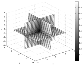
Figure 3: Normalized minimum time function with a control of norm 2.

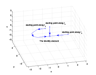
Figure 4: Optimal trajectories to the identity element starting from different points on each of the axes.

We use standard numerical tools from computational geometry to obtain a triangulation of the chosen subset of the algebra visualized as a region in $\mathbb{R}^{3}$ (since $\mathfrak{su}(2)$ is isomorphic to $\mathbb{R}^{3}$). Performing the value iteration mentioned in Section 5 the resulting value function is shown in Fig 3. Lighter shading at a point indicates a larger value of the minimum time function at that location. The stopping criteria used in the algorithm designed is as follows. At each step of the iteration the absolute change in the value function at all points on the mesh is computed. The maximum value of this change across the entire mesh is determined and a threshold value for this stopping metric, at which the algorithm should terminate, is set. This metric is indicated in Figure 5. Note that there are several different possibilities choices for a stopping criteria. We defer to future work the analysis of various possible stopping metrics and a detailed quantitative study of numerical convergence rates and error bounds.

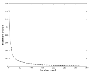
Figure 5: Maximum of the absolute change in the value function over the grid at each iteration.

The optimal controls are obtained using a discretized version of the verification theorem and from them we can obtain sample trajectories from various starting points as indicated in Fig 4. Note that this figure must be carefully interpreted since the mapping from this region into $SU(2)$ is not injective.

7 Conclusion

In this paper we introduced a rigorous framework for the numerical techniques involved in using the Dynamic Programming technique from optimal control theory for the control of quantum spin systems evolving on compact Lie groups. Numerical simulations were preformed by triangulation of the group which, due to the well studied numerical procedures available for tesselation of surfaces, enable better numerical speed and efficiency of implementation. In addition, the solution can be made more accurate at points of the group where such accuracy is desired (e.g around the origin in Fig. 3 where the solution is non differentiable). The dynamic programming methods provide a framework that can, in principle, be used for systems with an arbitrary number of qubits unlike limitations on the Lie theoretic methods. In addition, alternative numerical techniques that use the calculus of variations are subjected to issues in the entrapment at local minima - a drawback absent in the current approach.

The value function iteration methods when used on any grid, suffer from the curse of dimensionality and hence become intractable for higher dimensional systems. For instance, the number of spatial dimensions in a quantum spin $1/2$ system with $n$ qubits grows as ${4^{n}-1}$. Possible directions of future work may involve a study of methods such as fast marching [24] or meshless techniques to improve the speed of computations. Inspired by the dynamic programming framework in this article and the curse of dimensionality free approaches in [25], new methods are currently being developed for reduced dimensionality approximation techniques to quantum control.

There exist classes of control problems such as those involving quantum systems with bounded controls and drift for which the value function is discontinuous. Viscosity solution techniques for such discontinuous cost functions may be used to provide the technical framework for the use of impulsive controls in the dynamic programming approach to quantum control.

8 Acknowledgement

This research was supported by the Australian Research Council. The authors would also like to thank the anonymous reviewer for helpful comments.

References

- [1] R. B. N. Khaneja, S. J. Glaser, Time optimal control in spin systems, Phys. Rev. A 63 (2001) 032308.
- [2] N. Khaneja, T. Reiss, B. Luy, S. J. Glaser, Optimal control of spin dynamics in the presence of relaxation, Journal of Magnetic Resonance 162 (June 2003) 311–319(9).
- [3] G. Dirr, U. Helmke, K. Hüper, M. Kleinsteuber, Y. Liu, Spin dynamics: A paradigm for time optimal control on compact lie groups, Journal of Global Optimization 35 (3) (2006) 443–474.
- [4] A. Carlini, A. Hosoya, T. Koike, Y. Okudaira, Time-optimal quantum evolution, Physical Review Letters 96 (6) (2006) 60503.
- [5] M. A. Nielsen, M. R. Dowling, M. Gu, A. C. Doherty, Optimal control, geometry, and quantum computing, Physical Review A (Atomic, Molecular, and Optical Physics) 73 (6) (2006) 062323.
- [6] M. Nielsen, M. Dowling, M. Gu, A. Doherty, Quantum computation as geometry, Science 311 (5764) (2006) 1133–1135.
- [7] D. D’Alessandro, M. Dahleh, Optimal control of two-level quantum systems, IEEE Transactions on Automatic Control 46 (6) (2001) 866–876.
- [8] U. Boscain, P. Mason, Time minimal trajectories for a spin 1/2 particle in a magnetic field, Journal of Mathematical Physics 47 (6) (2006) 062101.
- [9] S. Sridharan, M. James, Minimum time control of spin systems via dynamic programming, in: Proceedings of the IEEE Conference on Decision and Control, IEEE, 2008.
- [10] S. Sridharan, M. Gu, M. R. James, Gate complexity using dynamic programming, Physical Review A (Atomic, Molecular, and Optical Physics) 78 (5) (2008) 052327.
- [11] D. Kirk, Optimal Control Theory: An Introduction, Courier Dover Publications, 2004.
- [12] D. Bertsekas, Dynamic Programming and Optimal Control, Athena Scientific, 1995.
- [13] A. Bryson, Y. Ho, Applied optimal control: optimization, estimation, and control, Taylor & Francis, 1975.
- [14] M. Bardi, I. C. Dolcetta, Optimal control and viscosity solutions of Hamilton-Jacobi-Bellman equations, Boston: Birkhauser, 1997.
- [15] Crandall, Some properties of viscosity solutions of Hamilton-Jacobi equations, Trans. AMS 282 (1984) 487–502.
- [16] D. Azagra, J. Ferrera, F. López-Mesas, Nonsmooth analysis and Hamilton–Jacobi equations on Riemannian manifolds, Journal of Functional Analysis 220 (2) (2005) 304–361.
- [17] D. Azagra, J. Ferrera, B. Sanz, Viscosity solutions to second order partial differential equations on Riemannian manifolds, i.
- [18] C. Mantegazza, A. Mennucci, Hamilton–Jacobi equations and distance functions on Riemannian manifolds, Applied Mathematics and Optimization 47 (1) (2002) 1–25.
- [19] P. Lions, Generalized solutions of Hamilton-Jacobi equations.
- [20] J. Munkres, Elementary Differential Topology, Princeton University Press, 1973.
- [21] H. Nijmeijer, A. Van der Schaft, Nonlinear dynamical control systems, Springer, 1990.
- [22] H. Kushner, P. Dupuis, Numerical Methods for Stochastic Control Problems in Continuous Time, Springer Verlag, Berlin-NY, 1992.
- [23] W. Fleming, H. Soner, Controlled Markov Processes and Viscosity Solutions, Springer Verlag, Berlin-NY, 2006.
- [24] R. Kimmel, J. Sethian, Computing geodesic paths on manifolds (1998).
- [25] W. McEneaney, A curse-of-dimensionality-free numerical method for solution of certain HJB PDEs, SIAM Journal on Control and Optimization 46 (4) (2008) 1239–1276.