The interval description of dynamics of celestial bodies in the planetary problem

Abstract

The interval approach to computation of dynamics of celestial bodies in the planetary problem has been considered. It is based on the refusal from idealization of infinitely high resolving capacity of measuring tools, and forms an absolutely exact algorithm free of round-off error accumulation effect. The possibilities of the proposed approach are shown by the examples of Kepler’s Problem and the problem of stability of the Solar system major planets for time interval of 6 billion years. The comparison of the interval and classical predictions of Kepler’s particle location in Kepler’s orbit provides support for the effect predicted by the theory, namely - conservation of the interval within which the values of difference of interval and classical coordinates lay with time. The computational results of the Solar system major planet orbital dynamics agree with the results obtained with the classical approach.

I Introduction

The interval-discrete concept of dynamics of point systems has been formulated in the paper (b1, ). The study is based on the refusal of idealization of an infinitesimal error of observations and calculations that is on the property of the limited resolving capacity of measuring tools and measurement processing facilities, which is not considered obviously in classical (trajectory) concept of motion. In the paper (b2, ) the interval description of macro bodies motion is applied to the planetary problem. The numerical computations of the Solar system planetary orbit evolution for time intervals of about 500-million years are performed in the study with the help of interval equations. The computations have verified the results obtained by classical methods, and have enabled to make a conclusion that the proposed interval approach is applicable for solving the problem of many bodies.

This paper presents the continuation of the study having been begun in (b2, ). The study objective is to completely realize and show the advantages of the interval approach as applied to the planetary problem and, thereby, to lay the groundwork for experimental check of the equations of the interval theory.

In this connection we remind (b1, ; b2, ) that formally the interval equations are a system of integer mappings of recurrent-type obtained by a special procedure of quantization of the time and spatial continuums of the system and the intervals of its dynamic variables. The feature of these mappings lies in the fact that they form an absolutely exact computational algorithm free of the effect of the round-off error accumulation. In this case it is possible to carry out computations with an unlimited number of iterations. The other feature of these mappings is a reasonable simplicity significantly reducing amount of computations in comparison with the classical approach. In the paper the mentioned features are illustrated by the examples of Kepler’s Problem and the problem of stability of the Solar system for cosmogonic times.

Kepler’s Problem is of interest as a basic problem. In particular, it allows demonstrating the interval tube effect (b2, ). Its manifestation is that the values of deviations of variable interval centers from their classical values lies in a strictly fixed interval the width of which does not exceed the initially preset width of interval variables. Classically it means that precision of the interval prediction for Kepler’s particles dynamics remains a constant value irrespective of "integration" duration. It is natural that the real reliability of such prediction will be limited by the time of system’s fall outside the limits of its «horizon of predictability» (b3, ). In this connection the interval dynamics in contrast to the classical dynamics in which there is no concept of "horizon of predictability» at all, allows to exactly estimate the "lifetime" of theoretical prediction, which is always finite in practice.

Kepler’s Problem allows demonstrating one more important property of the interval dynamics. That is ability of the interval tube for closing if the corresponding classical trajectory represents a closed phase curve. The uniqueness of this property is manifested by its inhesion to particularly numerical result, i.e. it means an absolutely exact recurrence of numerical parameters of the tube through one or several turns of a particle.

And, at last, there is one more interesting effect, which is demonstrated by the example of Kepler’s Problem. An interval particle alongside with an orbital moment has its own kinetic moment (spin). This effect is one of consequences of the interval nature of physical system space. It is conditioned by the fact that an interval particle in contrast to a classical one has the status of not a mathematical point, but a physical one. In other words the particle has finite size (determined by the width of intervals of the problem spatial variables) and, as a consequence, possesses its own moment of an impulse.

Freedom of the effect of round-off error accumulation allows successful solving of particularly academic problems alongside with practical ones. One of the problems is a study of a dynamic stability of the Solar system major planets. Difficulty of its solution is caused, first of all, by long-term character of the required prediction of the planets motion assuming carrying out the computations with time intervals of the Solar system age order. In the present work such computations are made for a time interval of six billion years. The obtained results agree with the results obtained earlier within the limits of the classical approach as for external planets (b7, ; b6, ; b4, ; b5, ), so as for internal planets (b7, ; b4, ; b5, ).

II Kepler’s problem

Let’s consider an interval statement of Kepler’s Problem in the space of polar coordinates presenting Hamiltonian of a classical analogue of the system under consideration in the following form:

$$H=\frac{1}{2}(p_{r}^{2}+\frac{p^{2}_{\varphi}}{r^{2}})-\frac{\mu}{r}.\\ (p_{\varphi}=c=\textrm{const})$$ (1)

In order to take into account the limited resolving capacity of the instrumental observation facilities and to pass to the interval description of the system dynamics (1), we introduce following to (b1, ) quantized spaces of its variables in the form of lattices with the following periods: $\rho$ - for radius $r$, $\sigma$ - for angle $\varphi$, $\upsilon$ - for impulse $p_{r}$ and $\vartheta$ - for time $t$. The designated periods will characterize the resolving capacity of corresponding observation procedures at the theoretical level. Thus the motion of a particle is described by not real numbers, but integer interval of coordinates $R_{n}=R(T_{n}),\Phi_{n}=\Phi(T_{n})$, impulse $P^{r}_{n}=P_{r}(T_{n})$ and time $T_{n}$ in the following form

$$\begin{array}[]{l}R_{n}=r_{n}+[-N,N],\\ \Phi_{n}=\varphi_{n}+[-N,N],\\ P^{r}_{n}=p_{n}+[-N,N],\\ T_{n}=[nN,nN+2N],\\ \end{array}$$ (2)

where $n=0,1,2,...$ - the number of the temporary variable lattice site with period $\tau=\vartheta N$, and $N\gg 1$ - the interval (integer) number.

According to (2) the state of the considered system is localized not in a point but in a multidimensional interval with the following absolute values of the half-width: $\alpha_{r}=\rho N$ - on variable $r$, $\alpha_{\varphi}=\sigma N$ - on variable $\varphi$, $\beta_{r}=\upsilon N$ - on variable $p_{r}$ and $\tau$ - on variable $t$. In terms of classical representations these values of half-width can be interpreted as the characterization of the numerical description of system. At that the given "precision" does not vary while the specified multidimensional interval moves with time in the quantized phase space forming an interval tube. Later we shall show that every such tube contains at least one classical trajectory.

As follows from the theory (b1, ), the designated values of the half-width are connected with the maximum velocities of change of the system generalized coordinates and impulses by ratios

$$\alpha_{r}=\tau V_{r},\\ \alpha_{\varphi}=\tau V_{\varphi},\\ \beta_{r}=\tau W_{r},$$ (3)

where $V_{r}\geq|dr/dt|_{\textrm{max}},\ V_{\varphi}\geq|d\varphi/dt|_{\textrm{max}},\ W_{r}\geq|dp_{r}/dt|_{\textrm{max}}$. At that the equations of dynamics for the integer centers $r_{n},\varphi_{n}$ and $p_{n}$ of the intervals (2) can be written down in the form of (b9, )

$$\begin{array}[]{l}r_{n+1}=r_{n}+[w\tilde{p}_{n}],\\ p_{n+1}=[\tilde{p}_{n+1}],\\ \varphi_{n+1}=[\tilde{\varphi}_{n+1}],\end{array}$$ (4)

where

$$\tilde{p}_{n+1}=p_{n}+\frac{\tau}{\upsilon}\left(-\frac{\mu}{\rho^{2}r^{2}_{n}}+\frac{c^{2}}{\rho^{3}r^{3}_{n}}\right),$$

$$\tilde{\varphi}_{n+1}=\varphi_{n}+\frac{\tau}{\sigma}\left(\frac{c}{\rho^{2}r^{2}_{n}-I}\right),$$

$$I=I_{0}+\delta\sum_{m=0}^{n}\sin(\sigma\varphi_{m}),$$

$$w=W_{r}\tau/V_{r}.$$

Here symbol $[x]$ (b1, ; b2, ) means the procedure of a round-off of real number $x$ up to the nearest integer, and function $I$ where $I_{0}$ and $\delta$ are the constants defined by the problem intervalization parameters, means the inertia moment of an interval particle. The occurrence of $I$ in the equation for $\varphi_{n}$ of the system (4) is caused by the fact that the interval particles have spin, that, in its turn, and as is mentioned above, is a consequence of finiteness of the localization area size of the interval particles. The detailed discussion of this effect is beyond the problem of this work. It will be an objective of a special paper.

Let’s apply the equation system (4) to calculate the motion of the particle over the closed orbit taking for definiteness $\mu=1,c=1,e=0.3$ ($e$ - eccentricity). Perform the calculations with step $\tau=0.07238$ that is $\sim$ 0.01 of the motion period over the selected orbit. Take $N=10^{7},V_{r}=0.303,W_{r}=0.52,V_{\varphi}=1.71,I_{0}=1.3\times 10^{-4},\delta=1.5\times 10^{-5}$ for the specified parameters. In this connection according to (3) the half-width of the interval of particle localization in the space shall not exceed $\alpha_{r}\approx 0.022$.

The results of calculations are presented in Figures 1-3. Fig.  1 shows the performance of full energy conservation laws and the kinetic moment of system. The figure presents the relative fluctuations of current energy values $\Delta E/|E|$ and kinetic moment $\Delta c/c$ for time interval of $2.4\times 10^{6}$ periods. These fluctuations are computed with the following formulas:

$$\Delta E=E_{\textrm{int}}-E,$$

$$\Delta c=c_{\textrm{int}}-c,$$

where

$$E_{\textrm{int}}=\frac{1}{2}\left(\upsilon^{2}p^{2}_{n}+\frac{c^{2}}{\rho^{2}r^{2}_{n}}\right)-\frac{\mu}{\rho r_{n}},$$

$$c_{\textrm{int}}=\frac{\rho^{2}r^{2}_{n}}{\rho^{2}r^{2}_{n}-I}c,\\ \ E=-\frac{\mu^{2}(1-e^{2})}{2c^{2}}.$$

It follows from Fig. 1 that the designated fluctuations lay in strictly fixed intervals which do not vary with the course of time, and equal by the width to $\sim 0.008$ - for energy, and to $\sim 10^{-4}$ - for kinetic moment.

The Fig. 2 shows effect of an interval tube. Fig. 2 presents the time dependence of $\Delta x=x_{\textrm{int}}-x_{\textrm{kep}}$ and $\Delta y=y_{\textrm{int}}-y_{\textrm{kep}}$ characterizing the deviations of coordinates of the interval tube axis $x_{\textrm{int}}=\rho r_{n}\cos(\sigma\varphi_{n})$, $y_{\textrm{int}}=\rho r_{n}\sin(\sigma\varphi_{n})$ on the corresponding values of Kepler’s coordinates

$$x_{\textrm{kep}}=\frac{c^{2}}{\mu}\frac{\cos(\sigma\varphi_{n})}{1+e\cos(\sigma\varphi_{n})},$$

$$y_{\textrm{kep}}=\frac{c^{2}}{\mu}\frac{\sin(\sigma\varphi_{n})}{1+e\cos(\sigma\varphi_{n})}.$$

According to Fig. 2 these deviations do not fall outside the limits of the fixed intervals with the half-width $\alpha_{x}\approx 0.006$ and $\alpha_{y}\approx 0.012$, i.e. the specified values satisfy the condition of localization $\alpha_{x,y}<\alpha_{r}$. This implies that the classical (Kepler’s) trajectory all over does not fall outside the limits of the intervals predicted by the equations (4), and entirely lies inside the corresponding interval tube.

One more interesting property of the interval tube becoming apparent in case of periodic motions is its closability. In the example under analysis such closing is observed on a phase plane $r_{n},p_{n}$. As calculations show, for initial conditions

$$r_{0}=350790178,\ p_{0}=-20$$ (5)

the closing of the interval tube $R_{n},P^{r}_{n}$ (interval analogue of the classical trajectory $r,p_{r}$) occurs in 100 steps, i.e. in one turn of a particle. This result is illustrated in Table 1 where the values of quantum numbers $r_{n}$ and $p_{n}$ are calculated by means of (4) in the beginning of the motion and in 100 steps.

Figure 1: The time dependence between the relative quantities of full energy fluctuations ($\Delta E/|E|$) and the orbital kinetic moment ($\Delta c/c$) of Kepler’s particle.

Figure 2: The time dependence between the differences of the interval and classical values of Cartesian coordinates of Kepler’s particle.

Table 1: The time dependence of phase variables $r_{n}$ and $p_{n}$ on a periodic trajectory.

$n$	$r_{n}$	$p_{n}$
0	350790178	-20
1	352000368	9742590
2	354394531	19274116
…..	…………….	…………..
100	350790178	-20
101	352000368	9742590
102	354394531	19274116

As is obvious, coincidence of these values represents not an approximate result, but an absolutely exact numerical result. Such property is a distinctive feature of the motion interval description and in principle is not realized within the limits of classical calculation means.

The picture of the interval description of particle motion in Kepler’s Problem is not complete if not to concern one more aspect of the interval theory, namely, an estimation of particle position predictability horizon. As follows from (b1, ), occurrence of such characteristic as "lifetime" of the theoretical prediction in the interval theory is a direct consequence of the explicit accounting of the interval nature of physical system phase space. The elementary cell of such space contains not one but $2^{2s}$ points in the form of combinations of integer values of impulses and coordinates, the single-type variables in which can differ from each other by not more than one quantum. The beam $2^{2s}$ of interval tubes coming out of such cell (physical point) gives the reliable prediction of the current system state till the integration of intervals of all phase variables for each of variables keeps in the interval of width $4N$. At violation of this condition if only for one of the variables it is possible to speak about an output beyond the horizon of the system state predictability.

This is the formality of the problem. In order to characterize the problem practically, let us consider particular procedures carried out when estimating the horizon of Kepler’s particles position predictability. And by the example of these procedures we shall demonstrate technology.

Let’s previously notice that the phase space of the considered system represents section $p_{\varphi}=c$ and forms a three-dimensional lattice with periods $\rho,\upsilon$ and $\sigma$ for phase variables $r_{n},p_{n}$ and $\varphi_{n}$, accordingly. Hence, the elementary cell of such space is a cube with a one-quantum side. Let’s introduce an estimation of divergence of a beam of the trajectories coming out of this cell during the initial moment of time. We analyze all the possible combinations of trajectory pairs, and select that very pair in which the trajectories diverge with the maximum velocity. In this case we calculate the divergence time comparing coordinates $x_{\textrm{int,1}},y_{\textrm{int,1}}$ and $x_{\textrm{int,2}},y_{\textrm{int,2}}$ of each pair applying criterion

$$\Delta l\leq l_{\textrm{loc}},$$ (6)

where

$$\Delta l=\sqrt{(x_{\textrm{int,1}}-x_{\textrm{int,2}})^{2}+(y_{\textrm{int,1}}-y_{\textrm{int,2}})^{2}},$$

and $l_{\textrm{loc}}\approx 0.024$. This value of width of the interval of the spatial localization of the particle is selected on the basis of the computation results presented in Fig. 2.

As the first example consider the dynamics of $\Delta l$ for a beam of trajectory tubes coming out of the cell, one top of which corresponds to the initial condition (5). For this condition the result of computation of the time dependence of value $\Delta l$ is shown in Fig.  3a and corresponds to the pair

$$\begin{array}[]{l}r_{01}=350790178,\ p_{01}=-20,\ \varphi_{01}=-20,\\ r_{02}=350790179,\ p_{02}=-19,\ \varphi_{02}=-20.\end{array}$$ (7)

It follows from Fig. 3a, because of (6), that the particle position predictability horizon is in the order of $2.5\times 10^{5}$ periods of the orbit motion.

Estimating this result, it is well to bear in mind that it corresponds to the localization of the initial particle state in terms of a phase space elementary cell. In practice such high degree of localization is not always achievable. Taking into consideration the real possibilities of observation tools, we should expand the area of the system initial state localization to some set of elementary cells. Such roughening of the system description leads as a rule to reduction of the dynamics reliable prediction time. This effect is shown in Figs. 3b and 3c. At that Fig. 3b describes pair

$$\begin{array}[]{l}r_{01}=350790168,\ p_{01}=-20,\ \varphi_{01}=-20,\\ r_{02}=350790169,\ p_{02}=-19,\ \varphi_{02}=-20,\end{array}$$ (8)

and Fig. 3c describes pair

$$\begin{array}[]{l}r_{01}=350790228,\ p_{01}=-30,\ \varphi_{01}=-20,\\ r_{02}=350790227,\ p_{02}=-29,\ \varphi_{02}=-20.\end{array}$$ (9)

The elementary cell of pair (8) is ten (10) quanta apart from the cell of pair (7) over $r_{n}$. This cell is characterized by an essentially smaller predictability horizon (if compare with (7)) equal to $\sim 7\times 10^{3}$ periods of the particle. We have still smaller predictability horizon of $\sim 4.5\times 10^{3}$ periods for pair (9) being 50 quanta apart from pair (7) over $r_{n}$ and 10 quanta apart - over $p_{n}$.

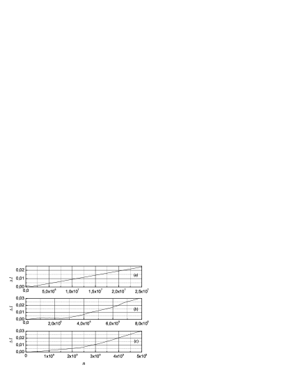
Figure 3: The time dependence of $\Delta l$ distance between Kepler’s particle locations belonging to two phase trajectories physically imperceptible in the initial moment.

III ORBITAL DYNAMICS OF PLANETS OF SOLAR SYSTEM

With the help of the interval equations (b2, ) numerical computation of motion of the major planets of the Solar system in the time interval of $6\times 10^{9}$ years has been made. Computations have been made with step $\tau=0.012$ year for $N=10^{9}$ . The masses of the planets have been taken from the system of constants IAU 1964. The initial rectangular heliocentric coordinates and velocities are related to the equator and correspond to the stage of 1949, Dec. 30.0 ET=JED 2433280.5. To study a long-term behavior of the planet orbits and their possible drift in a chaos zone, the time dependence of maximum eccentricities and inclinations of orbits for the interval centers of the mentioned variables has been calculated. The values of the half-widths of these intervals ($\alpha_{e}$ - for eccentricity and $\alpha_{i}$ - for inclination) are presented in Table  2. The maximum values have been selected from the set of values in time intervals of 6 million years, i.e. the technique similar to (b7, ) has been applied. The results of the calculations are presented in Figures 4-7.

Table 2: The values of half-widths of intervals of planetary orbit eccentricity ($\alpha_{e}$) and inclination ($\alpha_{i}$).

	$\alpha_{e}$	$\alpha_{i}$
Mercury	0.17
Venus	6.5E-3
Earth	0.0165
Mars	0.025	$\leq$5.0E-5
Jupiter	0.035
Saturn	3.5E-3
Uranus	3.0E-3
Neptune	4.5E-3
Pluto	0.045

Figs. 4 and 5 contain graphs of the above-mentioned dependences for the internal planets. They show a possible drift of orbit element values. Therewith the growth of the Mercury eccentricity (for which the zone of chaos is maximum) is limited (according to Fig.  4 and Table  2) by an interval of values the upper limit of which does not exceed $\sim$0.38. For the considered time interval this result agrees with the results obtained in (b7, ; b4, ; b5, ).

Figure 4: The time dependence of maximum orbit eccentricities of internal planets (for interval centers).

Figure 5: The time dependence of maximum orbit inclinations of internal planets (for interval centers).

Figure 6: The time dependence of maximum orbit eccentricities of external planets (for interval centers) : (a) - Jupiter, (b) - Saturn, (c) - Uranus, (d) - Neptune, (e) - Pluto.

Figure 7: The time dependence of maximum orbit inclinations of external planets (for interval centers) : (a) - Jupiter, (b) - Saturn, (c) - Uranus, (d) - Neptune, (e) - Pluto.

Computation of behavior of the external planets (Figs. 6 and 7) also coincides with that having been obtained earlier by the authors having been mentioned and also by (b6, ). The Uranus is an exception. For the Uranus, as seen from Fig.  6c, value $e_{max}$(with regard to the interval correction of Table 2) comes up to value of $\sim$0.178. Thus $e_{min}\approx 2\times 10^{-2}$ and as computations show, the Uranus eccentricity drift in this range has a random (stochastic) character, i.e. it can be regarded as a feature of chaotization of its motions and a motion of the external planets as a whole. A source of such chaotization is overlapping of the components of triple resonance of average motions of the Jupiter, Saturn and Uranus having been analyzed in the work of (b10, ). Other source is overlapping of resonant areas in the vicinity of the Uranus and Neptune orbits analyzed in (b11, ; b12, ). At the same time, the obtained result is still not sufficient for final conclusions. To get an unambiguous answer about the nature of motion of the external planets, additional computational investigations are necessary.

Completing the description of the results of this part of work, let us touch upon the problem of labor coefficient of the conducted computations. They have been carried out with the help of a personal computer with processor AMD Athlon 64 3400+. To improve the reliability, the computations have been conducted with extended precision having demanded the doubling of computation time. This time has been 1000 hours for time interval of 6 billion years ($5\times 10^{12}$ steps).

IV Conclusions

The conducted computations show the efficiency of the interval approach, its adequacy to the problems of celestial bodies’ dynamics. The interval means of motion description assure to obtain a solution in the defined strictly fixed interval of divergence from the classical trajectory (in case of periodic motions) and to attribute a unique property of absolutely exact closing. In solving the problems of long-term motion prediction the interval approach has one more advantage. Being free of round-off error accumulation effect it enables to computationally investigate the dynamics of planets in an arbitrary large time interval. At that the interval theory includes special computational procedure for estimating the horizon of the motion investigated aspects predictability.

The examples considered in the paper do not obviously solve all the problems related to the interval planetary dynamics. Along with academic problems, a set of problems being solved thanks to the creation of highly-precise ephemerides of planets and satellites is particularly actual. Moreover, the potential of the interval approach can be realized with the greatest efficiency in the class of applied problems.

It is obvious, that such realization is impossible without interest on the part of experts belonging to the appropriate application areas. And one of the problems of the present publication consists in turning the experts’ attention to perspectiveness of application of the interval theory methods and algorithms.

References

- (1) Petrov V. V., 2000, Fizicheskya mysl’ Rossii, no. 2, 15
- (2) Petrov V. V., 2004, Sol. Sys. Res., 38(5), 403
- (3) Lighthill J., 1986, Proc. Roy. Soc. Ser. A, 407, 35
- (4) Ito T., Tanikawa K., 2002, Proc. 8th IAU Asian-Pacific Reg. Meeting. Astron. Soc. Jap., 2, 45
- (5) Ito T., Tanikawa K., 2002, MNRAS, 336, 483
- (6) Kinoshita H., Nakai H., 1996, Earth, Moon, and Planets, 72, 165
- (7) Laskar J., 1994, A & A, 287, L9
- (8) Zeeman T. C., 1962, The topology of 3-Manifolds, M. K. Fort(ed), N. Y. 240
- (9) Sossinsky A. B., 1985, Acta Applic. Math., 5(2), 137
- (10) Murray N., Holman M., 1999, Science, 283, 1877
- (11) Guzzo M., 2005,Icarus, 174, 273
- (12) Guzzo M., 2006,Icarus, 181, 475