A two-step density-matrix renormalization-group study of coupled Luttinger liquids

Abstract

We report a two-step density-matrix renormalization-group computation of the equal-time single-particle Green’s function, the density-density correlations, and the low-frequency spectral weight function of a spinless fermion model in an anisotropic two-dimensional lattice at half-filling. We find that at weak couplings the density-density correlations have the universal decay of a Fermi liquid; the spectral weight function displays a sharp quasi-particle peak. But in the vicinity of a quantum critical point, these correlations strongly deviate from a Fermi liquid prediction and a pseudogap opens in the spectral weight function.

I Introduction

The metallic phase of interacting three-dimensional (3D) electron systems is described by the Fermi liquid theory (FLT) proposed by L. Landau landau . The Fermi liquid (FL) is a phase of matter in which low energy charged excitations and the long-distance behavior of correlation functions are essentially similar to those of the non-interacting electron system. They carry spin and are described as weakly-interacting quasi-particles. A microscopic justification of the FLT was given through the many-body perturbation theory agd ; nozieres and the renormalization group (RG) shankar ; chitov1 ; chitov2 . However neither the many-body perturbation theory nor the RG provide a complete demonstration of the emergence of a FL from an interacting electron model. The many-body perturbation theory neglects the competition between different channels and focuses only on the metallic phase. The RG analyses the flow of the interaction toward the FL fixed point, but it does not yield the quasi-particle spectra. Furthermore, both approaches are restricted to the weak-coupling regime. Indisputable FL behavior has been theoretically shown only for impurity models nozieres2 or model in infinite dimensions kotliar . Recent development into this difficult problem involved the use of string theory zaanen .

Electron-electron interactions have a dramatic effect in the one-dimensional (1D) metallic phase. No matter how small, they completely destroy the quasi-particles. An alternative to the FLT for 1D metals is Haldane’s haldane Luttinger liquid theory (LLT). The central assumption of the LLT is that the low-energy excitations and the long-distance behavior of correlation functions of 1D metals are similar to those of a model introduced by Luttinger luttinger . These excitations are density fluctuations which propagate with different velocities for the spin and charge. In a Luttinger liquid (LL), unlike a FL, the decay of the correlation functions is non-universal.

There is a significant interest in the question of the evolution of the Luttinger liquid when going from $D=1$ to $D>1$. This is relevant to the physics of quasi-one-dimensional organic conductors bourbonnais where pressure or temparuture can induce a crossover from an LL to a FL or an ordered phase. The dimensional crossover has been studied by various approaches. These include analytic continuation from D=1 to $D=1+\epsilon$ castellani , perturbative renormalization group (RG) on weakly-coupled LLbourbonnais or on 2D system with weak interaction shankar , functional integral boies , and generalized dynamical mean-field theory (DMFT) arrigoni ; bierman . These studies conclude to a FL ground state in 2D. However, Anderson and coworkers clarke ; strong have argued that, a different scenario due to strong interaction could take place. They pointed out that despite the RG being relevant, the resulting 2D system could nevertheless be a non-FL. The effects of the interactions could be so dramatic that if the transverse hopping is not strong enough, the electrons would remain confined in the chains. Coherent quasi-particles would form only when the transverse hopping exceeds a treshold. This issue has recently been reexaminated in the framework of the functional RG ledowski . A regime with confined coherence was predicted in the strong interaction regime. The non-FL mechanism suggested in Ref.clarke ; strong could occur for instance in the vicinity of a quantum critical point (QCP) where interaction effects are very strong.

In this paper, we use the two-step density-matrix renormalization group method moukouri-TSDMRG to study the possible emergence of FL and non-FL behaviors on an interacting electron model close to a QCP. Our results are consistent with a FL ground state in a 2D model for weak interactions. We also show that as a QCP is approached, the system enters a non-FL regime. This is captured by the behavior of the exponent $K$ of the density-density correlation which shows a strong renormalization towards its FL value for $V\lesssim 1$ and which is only weakly renormalized in the vicinity of the 1D quantum critical point. The evolution from a FL to a non-FL is also oberved in the low frequency spectral weight function.

II Model and Method

We concentrate on the following quasi-one-dimensional spinless fermion model on a finite lattice of size $L_{x}$, $L_{y}$ in the $x$, $y$ directions respectively:

$$H=-t_{x}\sum_{i_{x},i_{y}}(c_{i_{x},i_{y}}^{\dagger}c_{i_{x}+1,i_{y}}+h.c.)-\mu\sum_{i_{x},i_{y}}n_{i_{x},i_{y}}-$$

$$t_{y}\sum_{i_{x},i_{y}}(c_{i_{x},i_{y}}^{\dagger}c_{i_{x},i_{y}+1}+h.c.)+V\sum_{i_{x},i_{y}}n_{i_{x},i_{y}}n_{i_{x}+1,i_{y}}.$$ (1)

We are interested in the situation where the hopping parameter $t_{x}$ along the $x$ direction is far larger than the interchain hopping $t_{y}$, $t_{x}\gg t_{y}$. The interaction $V$ is chosen such that when $t_{y}=0$, we are in the LL phase, i.e., $V\lesssim 2t_{x}$. We will restrict ourselves to case where the electron density is at half-filling, $n_{0}=N_{e}/(L_{x}L_{y})=1/2$, where $N_{e}$ is the total number of electrons. It has been shown in Ref. moukouri-TSDMRG, that this type of anisotropic model may be studied using the density-matrix renormalization group (DMRG) method white . In this approach, the DMRG is applied in two steps.

In the first step, we use the DMRG to construct an approximate, yet well controlled, low-energy Hamiltonian ${\tilde{H}}_{0,i_{y}}$ for an isolated chain $i_{y}$ Hamiltonian

$$H_{0,i_{y}}=-t_{x}\sum_{i_{x}}(c_{i_{x},i_{y}}^{\dagger}c_{i_{x}+1,i_{y}}+h.c.)-\mu\sum_{i_{x}}n_{i_{x},i_{y}}+$$

$$V\sum_{i_{x}}n_{i_{x},i_{y}}n_{i_{x}+1,i_{y}}.$$ (2)

In order to allow interchain dynamics, ${\tilde{H}}_{0,i_{y}}$ is obtained by targeting the ground state of the nominal filling $N_{ex}/L_{x}=1/2$, where $N_{ex}$ is the number of electrons on the chain $i_{y}$. We also target ground states of $N_{ex}\pm 1$, $N_{ex}\pm 2$, $N_{ex}\pm 3$,… until the lowest state of a sector $N_{ex}\pm k$ is higher than the highest state kept in the $N_{ex}$ sector.

In the second step, the full 2D Hamiltonian (1) is projected onto the basis constructed from the tensor product of the single-chain eigenfunctions; this projection yields an effective one-dimensional Hamiltonian for the 2D lattice,

$$\tilde{H}\approx\sum_{i_{y}}\tilde{H}_{0,i_{y}}-t_{y}\sum_{i_{y}}(\tilde{c}_{i_{y}}^{\dagger}\tilde{c}_{i_{y}+1}+h.c.).$$ (3)

$\tilde{H}_{0,i_{y}}$ is diagonal, its element are the DMRG eigenvalues. $\tilde{c}\textbf{{}}_{i_{y}}^{\dagger}$, $\tilde{c}_{i_{y}}$, and $\tilde{n}_{i_{y}}$ are the renormalized operators in the single chain basis. These are vector operators made of local operators on each site of a chain $i_{y}$. It is clear that during the passage from the first to the second step, this method is different from the conventional DMRG in that the truncation is not done through the reduced density matrix. The truncation is done rather like in the real space RG method weinstein . But if $t_{y}$ remains small with respect to the energy width of the states kept, as in the Wilson approach for the Kondo problem wilson , this algorithm can retain high accuracy as we will show below.

	$16\times 17$	$32\times 33$	$64\times 65$
$\Delta E$	$1.950841$	$1.035854$	$0.534903$
$\delta\epsilon(t_{y}=0.05t_{x})$	$2.0\times 10^{-8}$	$<10^{-8}$	$2.4\times 10^{-7}$
$\delta\epsilon(t_{y}=0.1t_{x})$	$1.0\times 10^{-8}$	$4.6\times 10^{-7}$	$2.9\times 10^{-5}$

Table 1: Energy width $\Delta E$ of the $m_{2}=80$ states kept and error $\delta\epsilon$ in the ground-energy per site as function of the lattice size.

III Test on the non-Interacting case

Let us first analyze the performance of this DMRG algorithm for the case $V=0$ which enjoys an exact solution. The exact single particle energies and wave functions for open boundary conditions are respectively:

$$\epsilon_{{\bf k}_{l,m}}=-2t_{x}cosk_{x_{l}}-2t_{y}cosk_{y_{m}},$$ (4)

$$\psi_{{\bf k}_{l,m}}(i_{x},i_{y})=2\frac{sin(k_{x_{l}}i_{x})sin(k_{y_{m}}i_{y})}{\sqrt{(L_{x}+1)(L_{y}+1)}},$$ (5)

where $k_{x_{l}}=l\pi/(L_{x}+1)$, $k_{y_{m}}=m\pi/(L_{y}+1)$, $l=1,...,L_{x}$, $m=1,...,L_{y}$. The ground-state energy

$$E_{0}=\sum_{|{\bf k}_{l,m}|<k_{F}}\epsilon_{{\bf k}_{l,m}},$$ (6)

the single particle Green’s function between two points of coordinates $(i_{x},i_{y})$ and $(j_{x},j_{y})$,

$$g_{0}((i_{x},i_{y});(j_{x},j_{y}))=<c^{\dagger}_{i_{x},i_{y}}c_{j_{x},j_{y}}>,$$ (7)

and the density-density correlation between these points

$$C_{0}((i_{x},i_{y});(j_{x},j_{y}))=<(n_{i_{x},i_{y}}-n_{0})(n_{j_{x},j_{y}}-n_{0})>,$$ (8)

with $n_{\alpha_{x},\alpha_{y}}=c^{\dagger}_{\alpha_{x},\alpha_{y}}c_{\alpha_{x},\alpha_{y}}$, may be readily computed.

$$g_{0}((i_{x},i_{y});(j_{x},j_{y}))=\sum_{|{\bf k}_{l,m}|<k_{F}}\psi_{\bf k}^{*}(i_{x},i_{y})\psi_{\bf k}(j_{x},j_{y}),$$ (9)

$C_{0}((i_{x},i_{y});(j_{x},j_{y}))$ is obtained from $g_{0}((i_{x},i_{y});(j_{x},j_{y}))$ by the using Wick’s theorem.

In comparing the DMRG to this exact result, we emphasize that although the exact solution is trivial in momentum representation, for a real space method such as DMRG it remains a difficult challenge. However, unlike the exact solution, the DMRG can readily be extended to the case $V\neq 0$ without difficulty. In the DMRG, we kept up to $m_{1}=384$ states during the first step with up to $L_{x}=130$. For this value of $m_{1}$, the truncation error is virtually zero. Among the $4\times m_{1}^{2}$ states of the superblock, we kept a subset of up to $m_{2}=108$ states during the second step. These yield size dependent energy widths $\Delta E=\epsilon_{m_{2}}-\epsilon_{0}$, where $\epsilon_{0}$ and $\epsilon_{m_{2}}$ are respectively the lowest state and the highest state kept in a chain $i_{y}$ (see Table 1). The key to retain accuracy during the second step is to choose $t_{y}$ such that, $t_{y}\ll\Delta E$ for a given $L_{x}$. We show for instance in Table 1 the error in the ground state energies for $t_{y}=0.05t_{x}$ and $t_{y}=0.1t_{x}$ for $L_{x}\times L_{y}=16\times 17,~{}32\times 33,~{}64\times 65$. For $t_{y}=0.05t_{x}$, there is an excellent agreement with the exact energy for all sizes shown. Note that for the $16\times 17$ and $32\times 33$ lattices, the limitation to only 8 digits is due to the fact that we set the error to $10^{-6}$ in the diagonalization of the Hamiltonian. We could easily reach a smaller error without significant additional work. The agreement remains excellent for $t_{y}=0.1t_{x}$ except for a $64\times 65$ lattice. At this size, the difference between the DMRG and the exact energies is two orders of magnitude larger. The crossover temperature from 1D to 2D is given by $T_{X}\approx t_{y}/\pi$ bourbonnais , for finite size systems in the ground state, this translates to $\delta E\approx t_{y}$, where $\delta E$ is the size-dependent lowest excitation in 1D. We find that if $\delta E/t_{y}\lesssim 1$ and $\Delta E/t_{y}\approx 10$, the accuracy is almost independent of the system size. For instance, when $L_{x}\times L_{y}=32\times~{}33,64\times~{}65,130\times~{}131$, we find respectively, $\delta E=0.0951,~{}0.0483,~{}0.0240$. By respectively choosing $t_{y}=0.1,~{}0.05,~{}0.025$, we obtained $\delta\epsilon\lesssim 10^{-6}$. Hence, if we keep the ratios $\delta E/t_{y}$ and $\Delta E/t_{y}$ constant, we can access the 2D regime in large systems while retaining very good accuracy.

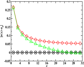
Figure 1: Density correlation $n(x)$ as function the position $x$ for the middle chain of 2D systems: DMRG with $V=0$, $t_{y}=0.05$ (circles); the exact result with $V=0$, $t_{y}=0.05$ (crosses); interacting 2D system with $V=1.5$, $t_{y}=0.1$ (triangles); single chain with $V=1.5$ (diamonds).

$\begin{array}[]{c@{\hspace{0.5in}}c}\lx@intercol\hfil\lx@intercol\\[-6.544pt] \includegraphics[width=113.81102pt,height=85.35826pt]{green02.eps}\hskip 14.22636pt\vspace{0.5cm}\includegraphics[width=113.81102pt,height=85.35826pt]{dens02.eps}\hfil\hskip 36.135pt\end{array}$ $\begin{array}[]{c@{\hspace{0.5in}}c}\lx@intercol\hfil\lx@intercol\\[-6.544pt] \includegraphics[width=113.81102pt,height=85.35826pt]{green2.eps}\hskip 14.22636pt\includegraphics[width=113.81102pt,height=85.35826pt]{dens2.eps}\hfil\hskip 36.135pt\end{array}$

Figure 2: (a),(b), respectively $g_{0}(x)$, $C_{0}(x)$ for a $64\times 65$ system, for $V=0$, $t_{y}=0.05$, the origin is on middle of the lattice, longitudinal direction: DMRG (circles), the exact result (crosses); transverse direction (only $g_{0}(x)$ is shown): DMRG (squares), exact result (pluses). (c),(d) respectively $g(x)$, $C(x)$ for a $63\times 63$ system, longitudinal direction: for $V=1.5$, $t_{y}=0$ (circles), for $V=1.5$, $t_{y}=0.1$ (squares); transverse direction (only $g(x)$ is shown): for $V=1.5$, $t_{y}=0.1$ (diamonds).

In order to limit the memory load, we computed the correlation functions in the central chain along the $x$ direction, $i_{y}=L_{x}/2+1$ (longitudinal direction), and in the central chain along the $y$ direction, $i_{x}=L_{x}/2$ (transverse direction). The local density $n_{0}(x)$ (Fig.1), $g_{0}(x)$ (Fig.2), and $C_{0}(x)$ (Fig.2) computed with the DMRG show a very good agreement with the exact result. We verified that the asymptotic behavior $x\gg 1$, $g_{0}(x)\propto 1/x$ and $C_{0}(x)\propto 1/x^{2}$ of the exact result is satisfied by the DMRG. For instance in Fig.2(a,b), for $g_{0}(x)$ the largest difference $\delta g_{0}$ between the DMRG and the exact result is seen in the tranverse direction at the largest distance $x=31$ for which $\delta g_{0}=0.0002$. The agreement is even better for $C_{0}(x)$, $\delta C_{0}(x)\approx 10^{-5}$ in the direction of the chains. For both the DMRG and the exact result, in the transverse direction, $C_{0}(x)$ for $x>3$ falls below $10^{-6}$ which is the error set in the diagonalization of the Hamiltonian. Hence, it was not shown. For this reason, we will exclusively concentrate on the correlation along the chains when analyzing the interacting case.

IV Density-density correlations

For $t_{y}=0$ and $V\neq 0$, there also exists an exact solution yang . The model is in a LL phase for $V<2t_{x}$ and in a charge density wave (CDW) phase for $V>2t_{x}$. In the LL phase, the asymptotic form of the Green’s function is $g_{1D}(x)\approx A_{g}/x^{1+\alpha}$, where $\alpha$ is the anomalous exponent. The dominant two-particle correlations are the density-density, $C_{1D}(x)=A_{c}/x^{2K}$ with $\alpha=(K+1/K)/2-1$. At $V=2t_{x}$, there is a 1D QCP. When open boundary conditions are applied, the sites at the ends generate strong Friedel oscillations. These oscillations decay very slowly from the ends and interfere with the normal density oscillations $C_{1D}(x)$. This behavior of the 1D system can be reproduced by the DMRG with extremely high accuracy.

When $t_{y}$ sets in, it is expected that either the system will be dominated by the single particle correlation, hence the ground state is a FL, or the density correlations $C_{1D}$ would freeze yielding an ordered two-dimensional CDW state. We did not find any evidence of CDW long-range order (LRO) when we start from the disordered 1D chain. It is important to note that the same method was used to study coupled spin chains and found LRO moukouri-TSDMRG as expected. Let us further discuss the reliability of this result. Since the DMRG is highly efficient in the interacting 1D case, the level of accuracy in 1D between the cases $V=0$ and $V\neq 0$ is comparable. Hence, studying the full Hamiltonian 1, which is no longer exactly solvable, with the DMRG is not more difficult than the $V=0$ case. The DMRG results of the 2D interacting case will be as good as those of the $V=0$ case, provided that $\Delta E$ does not decay sharply. When $V\neq 0$, an odd value of $L_{x}$ is chosen in order to not to frustrate the CDW correlations during the lattice growth caron . This choice also has the advantage of showing a sharp contrast for the behavior of the Friedel oscillations between 1D and 2D. We find for instance that in the LL phase for $V=1.5$, $L_{x}=63$, $\Delta E$ increases from its $V=0$ value $\Delta E=0.53$ to $0.95$. This implies that for the same value of $t_{y}$, the accuracy would be better for the $V=1.5$ case than for the $V=0$ case. However, for $L_{x}=63$ and $V=1.5$, $\delta E$ increases to $0.11$. For this reason, we have to increase the transverse hopping to $t_{y}=0.1$ in order to effectively be in the 2D regime. But since the ratio $\Delta E/t_{y}$ remains close to its $V=0$ value, the accuracy should not change. That is, we expect the error in the interacting Green’s function $\delta g\approx 10^{-4}$ and the error in the interacting density-density correlation function $\delta C\approx 10^{-5}$. This gives us a high degree of confidence in analyzing the properties of the 2D interacting system.

$\begin{array}[]{c@{\hspace{0.5in}}c}\lx@intercol\hfil\lx@intercol\\[-6.544pt] \includegraphics[width=113.81102pt,height=85.35826pt]{densv1.5t0.054.eps}\hskip 14.22636pt\vspace{0.5cm}\includegraphics[width=113.81102pt,height=85.35826pt]{densv1.5t0.054l130a.eps}\hfil\hskip 36.135pt\end{array}$

Figure 3: $C(x)$ for $V=1.5$, $t_{y}=0.054$: (a) $66\times 67$ (circles), $102\times 103$ (squares), and $130\times 131$ (diamonds) systems; (b) $L=102$ (1D, circles) and $102\times 103$ (squares); the vertical dotted lines show the limit of the retained data used for the extrapolations.

In the presence of $t_{y}$, the departure from 1D behavior which is characterized by strong oscillations of $n(x)$ can be seen in Fig.1. In the 1D systems these oscillations are present even in the bulk. For the 2D system, they vanish in the bulk, the density becomes uniform as in the case $V=0$. This is an indication that the dramatic departure from the free electron gas seen in the interacting 1D chain is strongly reduced by $t_{y}$. This is consistent with the relevance of $t_{y}$ or the irrelevance of $V$ (in 2D) found in perturbative RG. However, a crossover from a LL to a FL would be less apparent in $g(x)$ as seen in Fig.2(c). This is because in 1D, $\alpha$ varies only from $0$ when $V=0$ to $0.25$ at the QCP $V=2t_{x}$. At the same time the exponent $K=\pi/2arccos(-V/2t_{x})$, varies from $1$ to $0.5$. It is thus more favorable to use $C_{2D}(x)$ to analyze the crossover. $C_{2D}(x)$, shown in Fig.2(d), has a faster decay than in 1D. Unfortunately, the actual asymptotic behavior of $C_{2D}(x)$ is masked by the presence of the remnant of the Friedel oscillations at the ends. Unlike the 1D situation, in 2D they are $\pi$-dephased with $C_{2D}(x)$. Hence in order to access the asymptotic behavior in 2D, we reverted to even $L_{x}$ with odd $N_{ex}$, for which the Friedel oscillations are found to be less severe as shown in Fig.3.

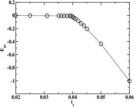
Figure 4: Ground state energy $E_{gs}$ with respect to the energy of disconnected chains for $V=0.75$ as function of $t_{y}$ for $64\times 65$ system.

$\begin{array}[]{c@{\hspace{0.5in}}c}\lx@intercol\hfil\lx@intercol\\[-6.544pt] \includegraphics[width=113.81102pt,height=85.35826pt]{densv0t0.025l130d.eps}\hskip 14.22636pt\vspace{0.5cm}\includegraphics[width=113.81102pt,height=85.35826pt]{densv0.75t0.038l130d.eps}\hfil\hskip 36.135pt\end{array}$ $\begin{array}[]{c@{\hspace{0.5in}}c}\lx@intercol\hfil\lx@intercol\\[-6.544pt] \includegraphics[width=113.81102pt,height=85.35826pt]{densv1.5t0.054l130d.eps}\hskip 14.22636pt\includegraphics[width=113.81102pt,height=85.35826pt]{densv2t0.073l130d.eps}\hfil\hskip 36.135pt\end{array}$

Figure 5: Linear fit of $C(x)$ for a $130\times 131$ systems: in all cases 1D DMRG (circles), exact (crosses), 2D DMRG (squares), exact (pluses); (a) $V=0$, $t_{y}=0.025$, (b) $V=0.75$, $t_{y}=0.038$; (c) $V=1.5$, $t_{y}=0.054$; (d) $V=2$, $t_{y}=0.073$. These values of $t_{y}$ are chosen so that ${\tilde{t}_{y}}\approx 1$.

Once in the 2D regime, in order to extract reliable correlation exponents, it is important to see how finite size effects affect the decay of correlation functions. In Fig.3(a), we show $C_{2D}(x)$ for $66\times 67$, $102\times 103$, and $130\times 131$ systems for $t_{y}=0.054$. $\delta E$ in these systems is respectively $0.1273$, $0.0675$, and $0.0531$. It can be drawn from the behavior of the $102\times 103$ and $130\times 131$ systems that in the regime $t_{y}\gtrsim\delta E$, aside from edges effects, finite size effects do not significantly affect the decay of the correlation functions in the 2D regime. We thus believe that the exponents of $C_{2D}(x)$ that we obtained are very close to their value in the thermodynamic limit. Even if edge effects are less dramatic when an odd $N_{ex}$ is chosen in an even $L_{x}$ system, they nevertheless strongly affect the extraction of the correlation exponent. In Fig.3(b) we show the range of the data used for the extraction of $K$. We arbitrary set $x\gtrsim 10$ from the origin and from the edge. For this choice it can be seen in Fig.3(b) that we are far enough from the upturn of $C_{2D}(x)$ caused by the edge.

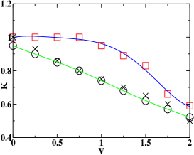
Figure 6: K as function of V: 1D DMRG (circles), 1D exact (crosses), 2D DMRG (squares).

Our calculations are made for small values of $t_{y}$, as pointed out earlier, it is expected that when $t_{y}\approx\delta E$, the 2D regime is reached. In order to make this argument more precise, we computed the ground-state energy $E_{gs}=E(t_{y})-E(t_{y}=0)$ as function of $t_{y}$. Two regimes, shown in Fig.4, are observed. When $t_{y}\lesssim\rho\delta E$, $E_{gs}$ remains nearly equal to the energy of disconnected chains. It would be expected that in this regime, the system will essentially have a 1D behavior. But when $t_{y}\gtrsim\rho\delta E$, the system gains energy with respect to disconnected chains. This is an indication that the system has entered the 2D regime. The typical value of $\rho$ is about $0.5$ for the values of $V$ we investigated.

Since we wish to analyze the effects of $V$ on the 2D system, we must be careful to avoid a spurious 2D to 1D crossover which is related to finite size effects. This occurs when we increase $V$. Starting at a relatively small value of $t_{y}$ and $V$ for which the condition $\delta E\lesssim t_{y}$ is satisfied for a given size, if we increase $V$ and keep $t_{y}$ constant, we can reach a regime where $t_{y}\ll\delta E$. Hence, we artificially enter an 1D regime. This is clearly a spurious effect due to the finite size of the system. In the thermodynamic limit, $\delta E\rightarrow 0$, hence, this situation never occurs for any finite $t_{y}$. This problem can be avoided by fixing the ratio ${\tilde{t}_{y}}=\frac{t_{y}}{\delta E}$ instead of $t_{y}$. This means that we compensate for the variation of $\delta E$ induced by $V$ by increasing $t_{y}$ so that we keep the system in the 2D regime.

In Fig.5 we show the decay of $C_{1D}(x)$ and $C_{2D}(x)$ for $V=0,~{}0.75,~{}1.5,~{}2$ in a $130\times 131$ system. $t_{y}$ is adjusted so that ${\tilde{t}_{y}}\approx 1$. Therefore, we are in the 2D regime of the model. It is important to stress that, if in that case a 1D like behavior is observed, this would be a genuine thermodynamic behavior of the system induced by the interactions. Fig.5(a) shows that the $V=0$ case in 1D and 2D are consistent with $1/x^{2}$ decay. In Fig.5(b), it can be seen that the 1D data deviate from the $1/x^{2}$ decay. On the other hand, the 2D behavior remains similar to the $V=0$ case. This is consistent with the LL nature of the 1D system and predictions of a FL ground state in 2D for mild interactions. When $V$ is further increased we find in Fig.5(c),(d) that the 2D results deviate from the FL behavior as well. Since there is no evidence of CDW LRO, this suggests the existence of an unconventional metallic state in 2D. A non-linear fit to these data yielded $K$ which is displayed in Fig.6. Non-linear fit are known to yield many different solutions depending on the starting point. To avoid this problem, we first computed the 1D exponents by fixing the search range in the interval $[0,1]$. The computed DMRG exponent shown in Fig.(6) was generally in very good agreement with the exact result. Surprisingly, the larger discrepancy was observed at $V=0$. These 1D exponents were later used as the input in the 2D search. The result shows a strong renormalization of $K$ from its LL value towards its FL value for $V\lesssim t_{x}$. Then, it enters a non-FL regime with $K<1$ when $t_{x}\lesssim V\lesssim 2t_{x}$.

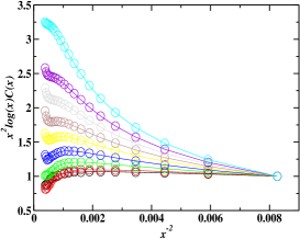
Figure 7: ${\tilde{C}}(x)=x^{2}log(x)C(x)$ relative to ${\tilde{C}}(x=11)$ as function of $x^{-2}$ for $V=0,0.25,0.5,0.75,1,1.25,1.5,1.75,2$ (from bottom to top); ${\tilde{t}_{y}}\approx 1$ in all cases; $t_{y}=0.025,0.03,0.035,0.038,0.042,0.048,0.054,0.067,0.073$ respectively from bottom to top.

In Fig.(7) in order to avoid the uncertainty related to the fit, the data on $C(x)$ were directly analyzed by studying ${\tilde{C}}(x)=x^{2}log(x)C(x)$, we added a factor $log(x)$ to the FL $x^{-2}$ decay to avoid a maximum that occurs in $x^{2}C(x)$ at large $x$ and $V>1.25$. We believe that this maximum is due to logarithmic corrections in the vicinity of the QCP. The factor $log(x)$ did not qualitatively modify the behavior of ${\tilde{C}}(x)$ when $V<1$. The plot of $\frac{{\tilde{C}}(x)}{{\tilde{C}}(11)}$ for values of ${\tilde{t}_{y}}\approx 1$, shows an evolution from $V=0$ to $V=2$. In the small $V$ regime, ${\tilde{C}}(x)$ is nearly flat. This is consistent with the FL physics. There is a downturn at large $x$ which is probably due to the influence of the edges. In the vicinity of the QCP ${\tilde{C}}(x)$ increases steadyly with increasing $x$. This clearly proves that $K$ is smaller than its FL value in this regime. It should be noted that the smallnest of $t_{y}$ implies that the 2D QCP remains very close to its 1D counterpart. Thus even if $V=2$ is not exactly at the 2D QCP, it lies very close to it. ${\tilde{C}}(x)$ evolves between these two limits as $V$ increases. This shows that the strong $V$ regime clearly departs from the FL picture.

V Low frequency spectrum

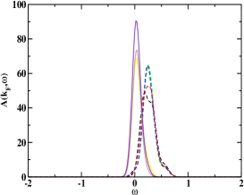
Figure 8: Spectral Weight function $A(k_{F},\omega)$ for $64\times 64$ systems respectively for increasing height for $V=0.75$: $t_{y}=0.005$ , $t_{y}=0.02$, $t_{y}=0.03$, and $t_{y}=0.0395$ (dotted lines), $t_{y}=0.04$, $t_{y}=0.05$, and $t_{y}=0.06$ (full lines).

A more direct information on the presence or lack of quasi-particles is given by the spectral weight function, $A({\bf k},\omega)=\sum_{n}\langle\Psi_{n}|a_{\bf k}^{\dagger}|\Psi_{0}\rangle\delta(\omega-\zeta_{n0})$, where $\Psi_{0}$ is the ground-state wave-function, $\Psi_{n}$ are the excited state wave functions with $N_{e}+1$ electrons, and $\zeta_{n0}$ are the excitation energies between the levels $0$ and $n$. The scope of finite frequency study will necessarily be limited to very low frequencies. The multiple RG steps in 1D and 2D have truncated out most of the Hilbert space of the system. We are left with a very tiny fraction of the total number of eigenfunctions and eigenvalues. The essential goal of this section is to show that $A({\bf k},\omega)$ near $\omega=0$ is consistent with our conclusions on $C_{2D}(x)$.

The DMRG can yield the low $\omega$ behavior of $A({\bf k},\omega)$ by targeting lowest states of sectors with $N_{e}$ and $N_{e}+1$ electrons. The low energy spectrum is then obtained by diagonalizing the reduced superblock of size $ms_{2}\times ms_{2}$ made of the two external blocks. As for the density-density correlation, we restricted ourselves to the central chain and used the following approximation, $A(k_{x},\omega)=\sum_{n}\langle\Psi_{n}|a_{k_{x}}^{\dagger}|\Psi_{0}\rangle e^{-\frac{(\omega-\zeta_{n0})^{2}}{\xi^{2}}}/\sqrt{\pi\xi^{2}}$, with $\xi^{2}=10^{-2}$. This means that we are not exactly at the Fermi point of the 2D systems. In presence of $t_{y}$, the Fermi point along $k_{y}=0$ is $(k_{F}+\delta k_{F},0)$, with $\delta k_{F}=Arccos(-ty/tx)-k_{F}$. Since $t_{y}/t_{x}\ll 1$, $\delta k_{F}$ is very small. The 1D Fermi point remains very close to the 2D Fermi surface.

$\begin{array}[]{c@{\hspace{0.5in}}c}\lx@intercol\hfil\lx@intercol\\[-6.544pt] \includegraphics[width=113.81102pt,height=85.35826pt]{Afermv0t0.05l64.eps}\hskip 14.22636pt\vspace{0.5cm}\includegraphics[width=113.81102pt,height=85.35826pt]{Afermv0.75t0.05l64.eps}\hfil\hskip 36.135pt\end{array}$ $\begin{array}[]{c@{\hspace{0.5in}}c}\lx@intercol\hfil\lx@intercol\\[-6.544pt] \includegraphics[width=113.81102pt,height=85.35826pt]{Afermv1.5t0.075l64.eps}\hskip 14.22636pt\includegraphics[width=113.81102pt,height=85.35826pt]{Afermv2t0.15l64.eps}\hfil\hskip 36.135pt\end{array}$

Figure 9: Spectral Weight function $A(k_{F},\omega)$ for $64\times 64$ systems: (a) $V=0$, $t_{y}=0.05$; (b) $V=0.75$, $t_{y}=0.05$; (c) $V=1.5$, $t_{y}=0.075$; (d) $V=2$, $t_{y}=0.15$.

As in the case of $C_{2D}(x)$, if $t_{y}\ll\rho\delta E$, $A({\bf k},\omega)$, the system will not show the 2D behavior. This is seen in spectra displayed in Fig.8 for $V=0.75$ and $L_{x}\times L_{y}=64\times 65$. When $t_{y}\lesssim 0.04$ (this is the point where a cusp is seen in $E_{gs}$), there is a pseudogap in $A({\bf k},\omega)$. This pseudogap is a 1D finite size effect. And as soon as the $t_{y}\gtrsim 0.04$, i.e the system enters the 2D regime following the criterion on $E_{gs}$, a quasi-particle peak appears in $A({\bf k},\omega)$. Hence, to some extent if L is large enough, increasing $t_{y}$ is equivalent to increasing the size of the system. This transition is very sharp. This is consistent the cusp observed in $E_{gs}$. In the 2D regimes the peak becomes sharper when $t_{y}$ is increased. This was observed for $0.04\lesssim t_{y}\lesssim 0.075$. When $t_{y}\gtrsim 0.075$, the peak was less sharp. This is due to the fact that for this value of $t_{y}$, the condition $t_{y}\ll\Delta E$ was no longer satisfied, hence we started loosing accuracy.

The spectra shown in Fig.9 are consistent with the conclusions drawn from $C(x)$. When $V\lesssim t_{x}$, there is a well defined quasi-particle peak at the Fermi energy for $k_{x}=k_{F}$. But when $t_{x}\lesssim V\lesssim 2t_{x}$, the peak shifts away from the Fermi energy; $A(k_{F},\omega)$ displays a quantum-fluctuation induced pseudogap which is a precursor of the CDW gap.

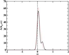
Figure 10: Spectral Weight function $A(k_{F},\omega)$ for $64\times 64$ systems for $V=1.5$: $t_{y}=0.075$ (full line), $t_{y}=0.1$ (dotted line).

The pseudogap observed between $1\lesssim V\lesssim 2$ exists for a finite range of $V$. This is for instance illustrated in Fig.(10) where $A(k_{F},\omega)$ is shown for $t_{y}=0.075$ and $t_{y}=0.1$. A pseudogap exists for both values of $t_{y}$. For $t_{y}=0.1$, there is a shift of the spectral weigth towards lower $\omega$. This is consistent with the possible crossover towards a FL at higher $t_{y}$.

VI Discussion and conclusion

In this work, we have shown that the two-step DMRG is a very useful tool for the study of quasi-1D models. This was illustrated in a spinless fermion model. We were able to obtain a very good accuracy on systems as large as $L\times(L+1)=130\times 131$. This is out of the reach of the conventional DMRG algorithm white . The essential difference with the coventional DMRG is the separation of the two energy scales of the Hamiltonian. The difficulty that arised in the interpretation of data was due not to accuracy but rather to the effects of open boundary conditions. In principle this could be avoided if periodic boundary conditions are used. However, we find that even periodic boundary conditions were not free of problem. When they are applied, the ground state is two-fold degenerate for even $N_{e}$. This means that in constructing the 1D Hamiltonian, additional effort should be made to keep tract of these multiplets. The computed low energy Hamiltonian for a single chain is then less accurate than with open boundary conditions.

The analysis of the correlation functions and of the low-energy spectral weight function revealed that a FL behavior occurs for small interactions. However, when the values of the interaction are close to the 1D quantum critical point, $V=2t_{x}$, the system behavior departs from that of a FL. A conservative view would be to infer this discrepancy to finite size effects. We did our best to disprove this possibility by showing that the decay of $C(x)$ is essentially identical for $102\times 103$ and $130\times 131$ systems for $V=1.5$. Given the nearly size independence of $K$ between $102\times 103$ and $130\times 131$, it is unlikely that the value $K=0.83$ at $V=1.5$ and ${\tilde{t}}\approx 1$ would significantly change to reach the FL value $K=1$ in the thermodynamic limit.

These results could be explained by the unconventional ideas raised by Anderson and coworkers clarke ; strong . When $0\lesssim V\lesssim 1$, the LL would be unstable against any small $t_{y}$. The resulting state is a FL. However, when $1\lesssim V\lesssim 2$, though $t_{y}$ is a relevant perturbation, there are no quasi-particles until $t_{y}$ exceeds a certain treshold.

- (1) L.D. Landau, Sov. Phys. JETP, 3, 920 (1957); L.D. Landau, Sov. Phys. JETP, 5, 101 (1957).
- (2) A. A. Abrikosov, L.P. Gorkov, and I.E. Dzyaloshinski, ”Methods of Quantum Field Theory in Statistical Physics”, Dover, New York (1963).
- (3) P. Nozières, ”Theory of Interacting Fermi Systems”, Benjamin, New York (1961).
- (4) R. Shankar, Rev. Mod. Phys. 66, 129 (1994).
- (5) G.Y. Chitov and D. Sénéchal, Phys. Rev. B 52, 13487 (1995); G.Y. Chitov and D. Sénéchal Phys. Rev. B 57, 1444 (1998).
- (6) G.Y. Chitov and A.J. Millis, Phys. Rev. bf B 64, 054414 (2001).
- (7) P. Nozières, J. Low. Temp. Phys. 17, 31 (1974).
- (8) A. Georges, G. Kotliar, W. Krauth, and M. J. Rozenberg, Rev. Mod. Phys. 68, 13 (1996).
- (9) M. Cubrovic, J. Zaanen, and K. Schalm, Science 325, 439 (2009).
- (10) F.D.M. Haldane, J. Phys. C 14, 2585 (1981).
- (11) J. M. Luttinger, J. Mat. Phys. 4, 1154 (1963).
- (12) C. Bourbonnais and L.G. Caron, Int. J. Mod. Phys. B 5, 1033 (1991).
- (13) C. Castellani, C. Di Castro, and W. Metzner, Phys. Rev. Lett. 72, 316 (1994).
- (14) D. Boies, C. Bourbonnais, and A.-M. S. Tremblay, Phys. Rev. Lett. 74, 968 (1995).
- (15) E. Arrigoni, Phys. Rev. Lett. 83, 128 (1999).
- (16) S. Biermann, A. Georges, A. Lichtenstein, and T. Giamarchi, Phys. Rev. Lett. 87, 276405 (2001).
- (17) D.G. Clarke, S.P. Strong, and P.W. Anderson, Phys. Rev. Lett. 74, 4499 (1995).
- (18) S.P. Strong and D.G. Clarke, J. Phys. Condens. Matter 8, 10089 (1996).
- (19) S. Ledowski and P. Kopietz, Phys. Rev. B 76, 121403 (2007).
- (20) S. Moukouri, Phys. Rev. B 70, 014403 (2004).
- (21) S.R. White, Phys. Rev. Lett. 69, 2863 (1992).
- (22) S. Drell, M Weinstein, and S. Yankielowicz, Phys. Rev. D 14, 487 (1976).
- (23) K.G. Wilson Rev. Mod. Phys.47, 773 (1975).
- (24) C.N. Yang and C.P. Yang, Phys. Rev. 150, 321 (1966).
- (25) L.G. Caron and C. Bourbonnais, Phys. Rev. B 66, 045101 (2002). 10089 (1996).