An introduced effective-field theory study of spin-1 transverse Ising model with crystal field anisotropy in a longitudinal magnetic field

Abstract

A spin-1 transverse Ising model with longitudinal crystal field in a longitudinal magnetic field is examined by introducing an effective field approximation (IEFT) which includes the correlations between different spins that emerge when expanding the identities. The effects of the crystal field as well as the transverse and longitudinal magnetic fields on the thermal and magnetic properties of the spin system are discussed in detail. The order parameters, Helmholtz free energy and entropy curves are calculated numerically as functions of the temperature and Hamiltonian parameters. A number of interesting phenomena such as reentrant phenomena originating from the temperature, crystal field, transverse and longitudinal magnetic fields have been found.

I Introduction

Ising model in a transverse field has been widely examined in statistical mechanics and condensed matter physics since the pioneering work of de Gennes deGennes who introduced it as a pseudo spin model for hydrogen-bonded ferroelectrics such as the $KH_{2}PO_{4}$ type. Following studies has been predicated that this semi-quantum mechanical model can be successfully applied to a variety of physical systems such as $DyVO_{4}$, $TbVO_{4}$ elliot and some real magnetic materials wong . From the theoretical point of view, transverse Ising model (TIM) has been investigated by a variety of techniques such as renormalization group method (RG) fisher_rg , effective field theory (EFT) saber_eft ; sarmento_eft ; Saber , cluster variation method (CVM) saxena_cvm , mean field theory (MFT) saxena_mf , pair approximation (PA) canko_pa and Monte Carlo simulations (MC) creswick_mc . In the previous works mentioned above, the authors focused their attention on the behavior of tricritical points but have not considered the effect of the crystal field (i.e. single ion anisotropy) in Hamiltonian describing the system.

However, there are a few studies in the literature that include the crystal field as well as the transverse field interactions. Recently, the effect of both the transverse field and the crystal field on the spin-$S$ Ising model with spins of magnitude $S$=1 have been studied and it is shown that TIM model presents a rich variety of critical phenomena. For example, Jiang et al. Jiang1 has studied the spin-1 TIM on a honeycomb lattice with a longitudinal crystal field and discussed the existence of a tricritical point at which the phase transition change from second-order to first order. By using the EFT with a probability distribution technique, Htoutou et al. Htoutou2 have investigated the influence of the crystal field on the phase diagrams of a site diluted spin-1 TIM on a square lattice. Similarly, Jiang have studied a bond diluted spin-1 TIM with crystal field interaction for a honeycomb lattice within the framework of the EFT with correlations Jiang2 . In these studies, the authors have reported the observation of a reentrant behavior on the system. Furthermore, in a series of papers Htoutou et al. Htoutou1 ; Htoutou3 have discussed the dependence of the behavior of the order parameters on the transverse and crystal fields, but they have restricted themselves on the second order transition properties. The effect of a longitudinal crystal field on the phase transitions in spin-$3/2$ and spin-$2$ transverse Ising model has been also examined for both honeycomb and square lattices by using the EFT with correlations wei_jiang1 ; wei_jiang2 . More recently, within the basis of EFT and MFT, Miao et al. Miao have studied the phase diagrams of a spin-1 transverse Ising model for a honeycomb lattice. They have obtained the first-order transition lines by comparing the Gibbs free energy.

An ordinary EFT approximation includes spin-spin correlations resulting from the usage of the Van der Waerden identities and provides results that are much superior to those obtained within the traditional MFT. However, the EFT approximations mentioned above are not sufficient enough to improve the results much. The reason may be due to the usage of a decoupling approximation that neglects the correlations between different spins that emerge when expanding the identities. According to us, the first-order transition lines obtained in Refs. Jiang1 ; Htoutou2 ; Jiang2 ; Htoutou1 ; Htoutou3 and Miao are incomplete, because the spin correlation functions such as $\langle S_{0}S_{1}\rangle$, $\langle S_{0}S_{1}S_{2}^{2}\rangle$ etc. can not be determined by using any decoupling approximation or in other words, by neglecting the correlations between different spins. In order to overcome this point, we proposed the IEFT approximation that takes into account the correlations between different spins in the cluster of considered lattice $(q=3)$ polat ; canpolat ; yuksel . Namely, the hallmark of the IEFT is to consider the correlations between different spins that emerge when expanding the identities and this method is superior to conventional mean field theory and the other EFT approximations in the literature. Therefore, it is expected that the calculation results will be more accurate.

As far as we know, there is not such a study which includes the longitudinal component of the magnetic field in addition to the crystal field and transverse magnetic field on the Hamiltonian. Thus, in the present work, we intended to investigate the thermal and magnetic properties of spin-1 TIM with crystal field under a longitudinal magnetic field on a honeycomb lattice within the framework of the IEFT. For this purpose, we investigated the proper phase diagrams, especially the first-order transition lines that include reentrant phase transition regions and we improved the results in Refs.Jiang1 ; Htoutou1 . We gave the numerical results for the behavior of the order parameters when the system undergoes a first or second order transition at a finite temperature. In addition, it would be interesting to see how the thermodynamic properties like entropy $S$ which has not been calculated before and Helmholtz free energy $F$ are effected by the crystal field as well as transverse and longitudinal magnetic fields. Hence, the numerical results are presented and compared with the literature.

The layout of this paper is as follows. In section II, we briefly present the formulations of the IEFT. The results and discussions are presented in section III. Finally, section IV contains our conclusions.

II Formulation

As our model we consider a two dimensional lattice which has $N$ identical spins arranged. We define a cluster on the lattice which consists a central spin labeled $S_{0}$, and $q$ perimeter spins being the nearest-neighbors of the central spin. The cluster consists of $(q+1)$ spins being independent from the value of $S$. The nearest-neighbor spins are in an effective field produced by the outer spins, which can be determined by the condition that the thermal average of the central spin is equal to that of its nearest-neighbor spins. The Hamiltonian of the spin-1 transverse model with crystal field in a longitudinal magnetic field is given by

$$H=-J\sum_{<i,j>}S_{i}^{z}S_{j}^{z}-D\sum_{i}(S_{i}^{z})^{2}-\Omega\sum_{i}S_{i}^{x}-h\sum_{i}S_{i}^{z},$$ (1)

where $S_{i}^{z}$ and $S_{i}^{x}$ denote the $z$ and $x$ components of the spin operator, respectively. The first summation in equation (1) is over the nearest-neighbor pairs of spins and the operator $S_{i}^{z}$ takes the values $S_{i}^{z}=0,\pm 1$. $J$, $D$, $\Omega$ and $h$ terms stand for the exchange interaction, single-ion anisotropy (i.e. crystal field) and transverse and longitudinal magnetic fields, respectively.

At first, we start constructing the mathematical background of our model by using the approximated spin correlation identities introduced by SáBarreto, Fittipaldi and Zeks Barreto

$$\langle\{f_{i}\}S_{i}^{\alpha}\rangle=\left\langle\{f_{i}\}\frac{Tr_{i}S_{i}^{\alpha}\exp{(-\beta H_{i})}}{Tr_{i}\exp{(-\beta H_{i})}}\right\rangle,$$ (2)

$$\langle\{f_{i}\}(S_{i}^{\alpha})^{2}\rangle=\left\langle\{f_{i}\}\frac{Tr_{i}(S_{i}^{\alpha})^{2}\exp{(-\beta H_{i})}}{Tr_{i}\exp{(-\beta H_{i})}}\right\rangle,$$ (3)

where $\beta=1/k_{B}T$ and $\alpha=z$ or $x$.

In order to apply the differential operator technique, we should separate the Hamiltonian (1) into two parts as $H=H_{i}+H^{{}^{\prime}}$. Here, one part denoted by $H_{i}$ includes all contributions associated with the site $i$, and the other part $H^{{}^{\prime}}$ does not depend on the site $i$. At this point, one should notice that $H_{i}$ and $H^{{}^{\prime}}$ do not commute with each other. We can write $-H_{i}$ as

$$-H_{i}=E_{i}S_{i}^{z}+D\left(S_{i}^{z}\right)^{2}+\Omega S_{i}^{x}+hS_{i}^{z},$$ (4)

where $E_{i}=J\sum_{j}S_{j}^{z}$ is the local field on the site $i$. If we use the matrix representations of the operators $S_{i}^{z}$ and $S_{i}^{x}$ for the spin-1 system then we can obtain the matrix form of equation (4)

$$-H_{i}=\left(\begin{array}[]{ccc}E_{i}+D+h&\Omega/\sqrt{2}&0\\ \Omega/\sqrt{2}&0&\Omega/\sqrt{2}\\ 0&\Omega/\sqrt{2}&-E_{i}+D-h\\ \end{array}\right).$$ (5)

In order to proceed further, we have to diagonalize $-H_{i}$ matrix in equation (5). The three eigenvalues are

$$\lambda_{1} = \frac{2c}{3}+\frac{2p}{3}\cos\left(\frac{\theta}{3}\right),$$

$$\lambda_{2} = \frac{2c}{3}-\frac{2p}{3}\cos\left(\frac{\pi-\theta}{3}\right),$$ (6)

$$\lambda_{3} = \frac{2c}{3}-\frac{2p}{3}\cos\left(\frac{\pi+\theta}{3}\right),$$

where

$$\theta = \arccos\left(\frac{\zeta}{p^{3}}\right),$$

$$\zeta = D\left(9E_{i}^{2}-\frac{9}{2}\Omega^{2}-D^{2}+18E_{i}h+9h^{2}\right),$$

$$p^{2} = 3E_{i}^{2}+3\Omega^{2}+D^{2}+6E_{i}h+3h^{2},$$

and the eigenvectors $\varphi_{k}$ of $-H_{i}$ corresponding to the eigenvalues in equation (II) are calculated as follows

$$\alpha_{k} = \pm\sqrt{1-\beta_{k}^{2}-\gamma_{k}^{2}},$$

$$\beta_{k} = -\frac{\left[E_{i}+(D+h-\lambda_{k})\right]}{\Omega/\sqrt{2}}\alpha_{k},$$

$$\gamma_{k} = -\frac{\left[E_{i}+(D+h-\lambda_{k})\right]}{\left[E_{i}-(D-h-\lambda_{k})\right]}\alpha_{k},$$

$$\varphi_{k}=\left(\begin{array}[]{c}\alpha_{k}\\ \beta_{k}\\ \gamma_{k}\\ \end{array}\right),\qquad k=1,2,3.$$ (7)

Hereafter, we apply the differential operator technique in equations (2) and (3) with $\{f_{i}\}=1$. From equation (2) we obtain the following spin correlations for the thermal average of a central spin for honeycomb lattice $(q=3)$ as

$$\langle S_{0}^{z}\rangle = \left\langle\prod_{j=1}^{q=3}\left[1+S_{j}^{z}\mathrm{sinh}(J\nabla)+(S_{j}^{z})^{2}\{\mathrm{cosh}(J\nabla)-1\}\right]\right\rangle$$ (8)

$$\times F(x)|_{x=0},$$

$$\langle S_{0}^{x}\rangle = \left\langle\prod_{j=1}^{q=3}\left[1+S_{j}^{z}\mathrm{sinh}(J\nabla)+(S_{j}^{z})^{2}\{\mathrm{cosh}(J\nabla)-1\}\right]\right\rangle$$ (9)

$$\times H(x)|_{x=0}.$$

By expanding the right-hand sides of equations (8) and (9) we get the longitudinal and transverse spin correlations as

$$m_{z}=\langle S_{0}^{z}\rangle = l_{0}+3k_{1}\langle S_{1}\rangle+3(l_{1}-l_{0})\langle S_{1}^{2}\rangle+3l_{2}\langle S_{1}S_{2}\rangle$$ (10)

$$+6(k_{2}-k_{1})\langle S_{1}S_{2}^{2}\rangle+3(l_{0}-2l_{1}+l_{3})\langle S_{1}^{2}S_{2}^{2}\rangle$$

$$+k_{3}\langle S_{1}S_{2}S_{3}\rangle+3(l_{4}-l_{2})\langle S_{1}S_{2}S_{3}^{2}\rangle$$

$$+3(k_{1}-2k_{2}+k_{4})\langle S_{1}S_{2}^{2}S_{3}^{2}\rangle$$

$$+(-l_{0}+3l_{1}-3l_{3}+l_{5})\langle S_{1}^{2}S_{2}^{2}S_{3}^{2}\rangle,$$

$$m_{x}=\langle S_{0}^{x}\rangle = p_{0}+3c_{1}\langle S_{1}\rangle+3(p_{1}-p_{0})\langle S_{1}^{2}\rangle+3p_{2}\langle S_{1}S_{2}\rangle$$ (11)

$$+6(c_{2}-c_{1})\langle S_{1}S_{2}^{2}\rangle+3(p_{0}-2p_{1}+p_{3})\langle S_{1}^{2}S_{2}^{2}\rangle$$

$$+c_{3}\langle S_{1}S_{2}S_{3}\rangle+3(p_{4}-p_{2})\langle S_{1}S_{2}S_{3}^{2}\rangle$$

$$+3(c_{1}-2c_{2}+c_{4})\langle S_{1}S_{2}^{2}S_{3}^{2}\rangle$$

$$+(-p_{0}+3p_{1}-3p_{3}+p_{5})\langle S_{1}^{2}S_{2}^{2}S_{3}^{2}\rangle.$$

Next, the average value of a perimeter spin in the system can be written as follows and it is found as

$$m_{1} = \langle S_{\delta}^{z}\rangle=\langle 1+S_{0}^{z}\mathrm{sinh}(J\nabla)+(S_{0}^{z})^{2}\{\mathrm{cosh}(J\nabla)-1\}\rangle$$ (12)

$$\times F(x+\gamma)|_{x=0},$$

$$\langle S_{1}\rangle=a_{1}\left(1-\langle(S_{0}^{z})^{2}\rangle\right)+a_{2}\langle S_{0}^{z}\rangle+a_{3}\langle(S_{0}^{z})^{2}\rangle,$$ (13)

where $\gamma=(q-1)A$ is the effective field produced by the $(q-1)$ spins outside the system and $A$ is an unknown parameter to be determined self-consistently. In the effective-field approximation, the number of independent spin variables describes the considered system. This number is given by the relation $\nu=\langle(S_{i}^{z})^{2S}\rangle$. As an example for the spin-1 system, $2S=2$ which means that we have to introduce the additional parameters $\langle(S_{0}^{z})^{2}\rangle$, $\langle(S_{0}^{x})^{2}\rangle$ and $\langle(S_{\delta}^{z})^{2}\rangle$ resulting from the usage of the Van der Waerden identity for the spin-1 Ising system. With the help of equation (3)

$$q_{z} = \langle(S_{0}^{z})^{2}\rangle$$ (14)

$$= \left\langle\prod_{j=1}^{q}\left[1+S_{j}^{z}\mathrm{sinh}(J\nabla)+(S_{j}^{z})^{2}\{\mathrm{cosh}(J\nabla)-1\}\right]\right\rangle$$

$$\times G(x)|_{x=0},$$

$$q_{x} = \langle(S_{0}^{x})^{2}\rangle$$ (15)

$$= \left\langle\prod_{j=1}^{q}\left[1+S_{j}^{z}\mathrm{sinh}(J\nabla)+(S_{j}^{z})^{2}\{\mathrm{cosh}(J\nabla)-1\}\right]\right\rangle$$

$$\times K(x)|_{x=0}.$$

Hence, we get the quadrupolar moments by expanding the right-hand sides of equations (14) and (15)

$$\langle(S_{0}^{z})^{2}\rangle = r_{0}+3n_{1}\langle S_{1}\rangle+3(r_{1}-r_{0})\langle S_{1}^{2}\rangle+3r_{2}\langle S_{1}S_{2}\rangle$$ (16)

$$+6(n_{2}-n_{1})\langle S_{1}S_{2}^{2}\rangle+3(r_{0}-2r_{1}+r_{3})\langle S_{1}^{2}S_{2}^{2}\rangle$$

$$+n_{3}\langle S_{1}S_{2}S_{3}\rangle+3(r_{4}-r_{2})\langle S_{1}S_{2}S_{3}^{2}\rangle$$

$$+3(n_{1}-2n_{2}+n_{4})\langle S_{1}S_{2}^{2}S_{3}^{2}\rangle$$

$$+(-r_{0}+3r_{1}-3r_{3}+r_{5})\langle S_{1}^{2}S_{2}^{2}S_{3}^{2}\rangle,$$

$$\langle(S_{0}^{x})^{2}\rangle = v_{0}+3\mu_{1}\langle S_{1}\rangle+3(v_{1}-v_{0})\langle S_{1}^{2}\rangle+3v_{2}\langle S_{1}S_{2}\rangle$$ (17)

$$+6(\mu_{2}-\mu_{1})\langle S_{1}S_{2}^{2}\rangle+3(v_{0}-2v_{1}+v_{3})\langle S_{1}^{2}S_{2}^{2}\rangle$$

$$+\mu_{3}\langle S_{1}S_{2}S_{3}\rangle+3(v_{4}-v_{2})\langle S_{1}S_{2}S_{3}^{2}\rangle$$

$$+3(\mu_{1}-2\mu_{2}+\mu_{4})\langle S_{1}S_{2}^{2}S_{3}^{2}\rangle$$

$$+(-v_{0}+3v_{1}-3v_{3}+v_{5})\langle S_{1}^{2}S_{2}^{2}S_{3}^{2}\rangle.$$

Corresponding to equation (12)

$$\langle(S_{\delta}^{z})^{2}\rangle=\langle 1+S_{0}^{z}\mathrm{sinh}(J\nabla)+(S_{0}^{z})^{2}\{\mathrm{cosh}(J\nabla)-1\}\rangle G(x+\gamma),$$ (18)

$$\langle S_{1}^{2}\rangle=b_{1}\left(1-\langle(S_{0}^{z})^{2}\rangle\right)+b_{2}\langle S_{0}^{z}\rangle+b_{3}\langle(S_{0}^{z})^{2}\rangle.$$ (19)

Details of calculation through (8-19) can be found in Appendix section. With the help of equations (II) and (7) the functions $F(x)$, $G(x)$, $H(x)$ and $K(x)$ in equations (8), (9), (14) and (15) can be calculated numerically from the relations

$$F(x)=\frac{1}{\sum_{n=1}^{s=3}\exp{(\beta\lambda_{n})}}\sum_{n=1}^{s=3}\langle\varphi_{n}|S_{i}^{z}|\varphi_{n}\rangle\exp{(\beta\lambda_{n})},$$ (20)

$$H(x)=\frac{1}{\sum_{n=1}^{s=3}\exp{(\beta\lambda_{n})}}\sum_{n=1}^{s=3}\langle\varphi_{n}|S_{i}^{x}|\varphi_{n}\rangle\exp{(\beta\lambda_{n})},$$ (21)

$$G(x)=\frac{1}{\sum_{n=1}^{s=3}\exp{(\beta\lambda_{n})}}\sum_{n=1}^{s=3}\langle\varphi_{n}|(S_{i}^{z})^{2}|\varphi_{n}\rangle\exp{(\beta\lambda_{n})},$$ (22)

$$K(x)=\frac{1}{\sum_{n=1}^{s=3}\exp{(\beta\lambda_{n})}}\sum_{n=1}^{s=3}\langle\varphi_{n}|(S_{i}^{x})^{2}|\varphi_{n}\rangle\exp{(\beta\lambda_{n})}.$$ (23)

The internal energy $U$ per site of the system can be obtained easily from the thermal average of the Hamiltonian in equation (1). Thus, the internal energy is given by

$$-\frac{U}{NJ}=\frac{q}{2}\langle S_{0}S_{1}\rangle+D\langle(S_{0}^{z})^{2}\rangle+\Omega\langle S_{0}^{x}\rangle+h\langle S_{0}^{z}\rangle,$$ (24)

where the correlation functions $\langle S_{0}S_{1}\rangle$, $\langle(S_{0}^{z})^{2}\rangle$, $\langle S_{0}^{x}\rangle$ and $\langle S_{0}^{z}\rangle$ are obtained from equation (A). With the use of equation (24), the specific heat of the system can be numerically determined from the relation

$$C_{h}=\left(\frac{\partial U}{\partial T}\right)_{h}.$$ (25)

The Helmholtz free energy of a system is defined as

$$F=U-TS,$$ (26)

which, according to the third law, can be written in the form Huang

$$F=U-T\int_{0}^{T}\frac{C}{T^{{}^{\prime}}}dT^{{}^{\prime}},$$ (27)

where the integral in the second term is entropy of the system according to the second law. First, we calculate the internal energy per site from equation (24). Then with the help of equation (25) we can carry out numerical integration and calculate the entropy and free energy of the system. Equations (10), (11), (13), (16), (17) and (19) are fundamental correlation functions of the system. When the right-hand sides of equations (8), (9), (14) and (15) are expanded, the multispin correlation functions can be easily obtained. The simplest approximation, and one of the most frequently adopted is to decouple these equations according to

$$\left\langle S_{i}^{z}(S_{j}^{z})^{2}...S_{l}^{z}\right\rangle\cong\left\langle S_{i}^{z}\right\rangle\left\langle(S_{j}^{z})^{2}\right\rangle...\left\langle S_{l}^{z}\right\rangle,$$ (28)

for $i\neq j\neq...\neq l$ decoupling . The main difference of the method used in this study from the other approximations in the literature emerges in comparison with any decoupling approximation (DA) when expanding the right-hand sides of equations (8), (9), (14) and (15). In other words, one advantage of the approximation method proposed by this study is that no uncontrolled decoupling procedure is used for the higher-order correlation functions.

For spin-1 Ising system with $q=3$, taking equations (10), (11), (13), (16), (17) and (19) as a basis, we derive a set of linear equations of the spin correlation functions which interact in the system. At this point, we assume that (i) the correlations depend only on the distance between the spins, (ii) the average values of a central spin and its nearest-neighbor spin (it is labeled as the perimeter spin) are equal to each other, and (iii) in the matrix representations of spin operator $\hat{S}$, the spin-1 system has the properties $(S_{\delta}^{z})^{3}=S_{\delta}^{z}$ and $(S_{\delta}^{z})^{4}=(S_{\delta}^{z})^{2}$. Thus, the number of the set of linear equations obtained for the spin-1 Ising system with $q=3$ reduces to twenty three and the complete set is given in Appendix.

If equation (A) is written in the form of a $23\times 23$ matrix and solved in terms of the variables $x_{i}[(i=1,2,...,23)(e.g.,x_{1}=\langle S_{0}^{z}\rangle,x_{2}=\langle S_{1}S_{0}\rangle,...,x_{23}=\langle(S_{0}^{x})^{2}\rangle)]$ of the linear equations, all of the spin correlation functions can be easily determined as functions of the temperature, effective field, crystal field and longitudinal magnetic field as well as transverse magnetic field which the other studies in the literature do not include. Since the thermal average of the central spin is equal to that of its nearest-neighbor spins within the present method then the unknown parameter $A$ can be numerically determined by the relation

$$\langle S_{0}^{z}\rangle=\langle S_{1}\rangle\qquad{\rm{or}}\qquad x_{1}=x_{4}.$$ (29)

By solving equation (29) numerically at a given fixed set of Hamiltonian parameters we obtain the parameter $A$. Then we use the numerical values of $A$ to obtain the spin correlation functions $\langle S_{0}^{z}\rangle$, $\langle S_{0}^{x}\rangle$ (longitudinal and transverse magnetizations), $\langle(S_{0}^{z})^{2}\rangle$, $\langle(S_{0}^{x})^{2}\rangle$ (longitudinal and transverse quadrupolar moments) and so on, which can be found from equation (A). Note that $A=0$ is always the root of equation (29) corresponding to the disordered state of the system. The nonzero root of $A$ in equation (29) corresponds to the long-range ordered state of the system. Once the spin correlation functions have been evaluated then we can give the numerical results for the thermal and magnetic properties of the system.

III Results and Discussions

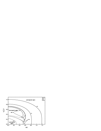
(a)

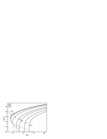
(b)

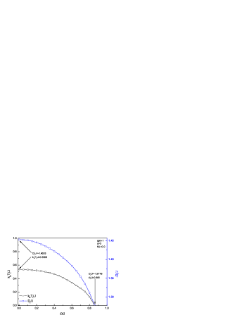
(c)

Figure 1: Phase diagrams of the spin-1 system with $h/J=0$ in (a) ($k_{B}T_{c}/J$-$\Omega/J$), (b) ($k_{B}T_{c}/J$-$D/J$) planes. The numbers on the curves denote the values of the crystal field $D/J$ and transverse field $\Omega/J$, respectively. (c) Transverse field dependencies of the tricritical temperature $k_{B}T_{t}/J$ and tricritical crystal field $-D_{t}/J$.

In this section, we can examine the ferromagnetic properties of the spin-1 TIM with crystal field under an applied longitudinal magnetic field on a honeycomb lattice using the IEFT. For this purpose, we focus our attention on the phase diagrams of the system in $(k_{B}T_{c}/J-\Omega/J)$ and $(k_{B}T_{c}/J-D/J)$ planes and investigate the whole phase diagrams by examining the numerical results for the thermal and magnetic properties. In order to plot the phase diagrams, we assume $\langle S_{0}^{z}\rangle=\langle S_{1}\rangle$ and the effective field $\gamma$ is very small in the vicinity of $k_{B}T_{c}/J$ and solve the set of linear equations in equation (A) numerically using the self-consistent relation corresponding to equation (29). In Figs. 1a and 1b, we plot the variation of the critical temperature with transverse field $\Omega/J$ and crystal field $D/J$, respectively. Fig. 1a shows the phase diagram in the $(k_{B}T_{c}/J-\Omega/J)$ plane with $h/J=0$ and for selected values of $D/J$, namely $-1.0,-1.3,-1.381,-1.382$ and $-1.4$. In this figure, we can call attention to the signs of an interesting behavior known as reentrant phenomena. In other words, when the crystal field strength is positive valued, the type of the transition in the system is invariably second order which is independent from transverse field value. On the other hand, if the crystal field value is sufficiently negative then we can expect to see two successive phase transitions. Solid and dashed lines in Fig. 1a correspond to the second and first order phase transition lines, respectively. Tricritical end points at which first and second order transition points meet are shown as white circles. In our calculations, we realized that one can observe reentrant behavior in the system for the values of $\Omega/J<0.861$ and $-1.4533<D/J<-1.0201$. For the values of $D/J\leq-1.382$ the transition lines exhibit a bulge which gets smaller as the value of $D/J$ approaches the value of $-1.4533$ which means that ferromagnetic phase region gets narrower. We have also examined the phase diagram of the present system in $(k_{B}T_{c}/J-D/J)$ plane with $h/J=0$ and for selected values of $\Omega/J$ such as $0,0.25,0.5,0.75,0.86,1.0$ and $1.1$. The numerical results are shown in Fig. 1b. Solid and dashed lines in Fig. 1b correspond to the second and first order phase transition lines, respectively. White circles denote tricritical points. As we can see from this figure, as the value of transverse field $\Omega/J$ increases starting from zero then the value of tricritical point decreases gradually and disappears for $\Omega/J>0.86$. If the transverse field value is greater than this value then we have only second order transitions in the system. These results show that the reentrant phenomenon originates from the competition between the crystal field $D/J$ and transverse field $\Omega/J$. Furthermore, the variation of the coordinates of the tricritical points $k_{B}T_{t}/J$ and $D_{t}/J$ as a function of transverse field $\Omega/J$ is illustrated in Fig. 1c. This figure shows that the tricritical points exist for $1.4333<-D_{t}/J<1.2776$ and $\Omega/J<0.861$. In addition, value of $k_{B}T_{t}/J$ and the absolute value of $D_{t}/J$ decreases as the value of transverse field increases and the tricritical temperature disappears at the critical value of the transverse field $\Omega_{t}/J=0.861$. All of the results mentioned above are in a good agreement with other works Saber ; Jiang1 ; Htoutou2 ; Jiang2 ; Htoutou1 ; Htoutou3 , but not with Miao .

(a)

(b)

(c)

(d)

Figure 2: Temperature dependencies of (a) longitudinal magnetization $m_{z}$, (b) transverse magnetization $m_{x}$, (c) longitudinal quadrupolar moment $q_{z}$ and (d) transverse quadrupolar moment $q_{x}$ for the spin-1 system on a honeycomb lattice with a fixed value of transverse field $\Omega/J=0.5$ and some selected values of crystal field $D/J=1.0,0,-0.5,-1.0,-1.25,-1.38$ and $-1.4$. The longitudinal magnetic field value is selected as $h/J=0$ and $0.1$ on the left and right panels, respectively. Dashed lines correspond to the first-order solutions.

In order to clarify the first-order phase transitions in the system we examine the variation of the order parameters with temperature such as the longitudinal and transverse magnetizations $m_{z}$ and $m_{x}$ together with the longitudinal and transverse quadrupolar moments $q_{z}$ and $q_{x}$. The effects of the crystal field on the behavior of the order parameters with a selected transverse field value $\Omega/J=0.5$ are shown in Fig. 2. Here, dashed lines correspond to the solutions of the first order transition. As we can see on the left panel in Fig. 2a, for the selected values of the crystal field $D/J=1.0,0,-0.5,-1.0$ and $-1.25$ with $h/J=0$ as the temperature increases, the longitudinal magnetization $m_{z}$ falls rapidly from its saturation magnetization value at $k_{B}T/J=0$ and decreases continuously in the vicinity of the transition temperature and vanishes at a critical temperature $T=T_{c}$. Besides, when we select the value of the crystal field such as $D/J=-1.38$ and $-1.4$ we observe two successive phase transitions. In other words, if we cool the system starting from a finite temperature $T>T_{c}$, the system undergoes a phase transition from paramagnetic to ferromagnetic phase at $T=T_{c}$. If we keep on cooling process then the second order transition at a finite temperature is followed by a first order transition at a lower temperature $T<T_{c}$. These results show the existence of reentrant phenomena. Furthermore, as the value of crystal field $D/J$ decreases then the second order transition temperature decreases and the first order transition temperature increases. On the left panel in Fig. 2b, we see the behavior of the transverse magnetization with temperature for some selected values of crystal field with $h/J=0$. For $D/J=1.0,0,-0.5,-1.0$ and $-1.25$ the transverse magnetization $m_{x}$ curves increase with the increase of the temperature and then show a cusp which increases in height as the value of the crystal field decreases at $T=T_{c}$ and decline as the temperature increases. Consequently, the transverse magnetization curves can be separated into two regions: the first is the nonmagnetic region in which $m_{z}=0$ and the second is the magnetic region in which $m_{z}\neq 0$. For $D/J=-1.38$ and $-1.4$ $m_{x}$ curves show a discontinuous behavior at the first order transition point. In Figs. 2c and 2d, the variation of the longitudinal and transverse quadrupolar moments with temperature are shown, respectively. The same crystal field $D/J$ values are used as in Figs. 2a and 2b. We see that the longitudinal quadrupolar moment $q_{z}$ decreases as the temperature increases and change abruptly at the second order transition temperature for $D/J=1.0,0,-0.5,-1.0$ and $-1.25$. In case of $D/J=-1.38$ and $-1.4$, $q_{z}$ curves exhibit two minima which correspond to the first and second order transition temperatures. In contrast to $q_{z}$ curves in Fig. 2 c, the transverse quadrupolar moment $q_{x}$ curves increases as the temperature increases and change abruptly at the second order transition temperature for $D/J=1.0,0,-0.5,-1.0$ and $-1.25$. For the values of crystal field $D/J=-1.38$ and $-1.4$ $q_{x}$ curves exhibit two maxima corresponding to the first and second order transitions in the system. When we apply a longitudinal magnetic field such as $h/J=0.1$ on the system, both the first and second order phase transition effects on the order parameters $m_{z}$, $m_{x}$, $q_{z}$ and $q_{x}$ are removed. This phenomenon can be clearly seen from the right hand side panels in Figs. 2a-2d.

(a)

(b)

(c)

(d)

Figure 3: Temperature dependencies of (a) longitudinal magnetization $m_{z}$, (b) transverse magnetization $m_{x}$, (c) longitudinal quadrupolar moment $q_{z}$ and (d) transverse quadrupolar moment $q_{x}$ for the spin-1 system on a honeycomb lattice with a fixed value of crystal field $D/J=-1.1$ and some selected values of transverse field $\Omega/J=0,0.5,0.75,0.9$ and $1.0$. $\Omega/J=0.25$ is also selected in (b). The longitudinal magnetic field value is selected as $h/J=0$ and $0.1$ on the left and right panels, respectively. Dashed lines correspond to the first-order solutions.

Next, the transverse field effect on the variation of the order parameters with temperature such as the longitudinal and transverse magnetizations $m_{z}$ and $m_{x}$ as well as the longitudinal and transverse quadrupolar moments $q_{z}$ and $q_{x}$ with $D/J=-1.1$ and $h/J=0$ can be seen on the left panels Fig. 3. Dashed lines represent the first order transition solutions. In Fig. 3a, we plot the longitudinal component of magnetization for selected values of transverse field $\Omega/J=0,0.5,0.75,0.9$ and $1$. As we can see on the left panel in Fig. 3a, as the transverse field $\Omega/J$ increases, critical temperature value approaches to zero and saturation value of $m_{z}$ decreases. Hence, we can say that applying transverse field $\Omega/J$ weakens the longitudinal component of magnetization. This is an expected result. However, two successive transitions (i.e. reentrant behavior) are observed on the longitudinal magnetization $m_{z}$ for $\Omega/J=0$. It is clear that applied transverse field $\Omega/J$ destructs the first order transition. On the left panel in Fig. 3b, we represent the effect of the transverse field $\Omega/J$ on the temperature dependence of $m_{x}$. In contrast to the situation in $m_{z}$, transverse field $\Omega/J$ strengthens the transverse component of magnetization. We note that, at zero transverse field the transverse magnetization $m_{x}$ is zero for the whole range of temperature. On the left panels in Figs. 3c and 3d, we present the effect of the transverse field $\Omega/J$ on the variation of the quadrupolar moments $q_{z}$ and $q_{x}$ with temperature, respectively. As we can clearly see from these plots, longitudinal quadrupolar moment $q_{z}$ has two minima while transverse counterpart $q_{x}$ has two maxima corresponding to the first and second order transitions for $\Omega/J=0$. Furthermore, applying any longitudinal magnetic field such as $h/J=0.1$ on the system, both the first and second order phase transitions are destructed. This behavior is illustrated on the right panels in Fig. 3. Hence, on the basis of these results (see the right panels in Figs. 2 and 3) we believe that the effects of the transverse field $\Omega/J$ are very different from those of the longitudinal counterpart $h/J$ because the origin of the transverse field is quantum mechanical and can produce quantum effects.

(a)

(b)

(c)

(d)

Figure 4: Entropy of the system as a function of temperature for $h/J=0$ and (a) $\Omega/J=0$ with some selected values of crystal field $D/J=0.5,0,-0.5,-0.75,-1.0,-1.4$ and $-1.44$, (b) $\Omega/J=0,0.5,0.75,0.9$ and $1.0$ with a fixed value of crystal field $D/J=-1.1$. (c) Temperature dependence of Helmholtz free energy of the system for $h/J=0$. The value of transverse field is fixed as $\Omega/J=0.0$ with some selected values of crystal field $D/J=0.5,0,-0.5,-1.0,-1.1,-1.32,-1.4$ and $-1.44$. (d) crystal field is fixed as $D/J=-1.1$ with five different values of transverse field $\Omega/J=0,0.5,0.75,0.9$ and $1.0$.

Finally in Fig. 4, we present the numerical results for the temperature dependence of entropy per site and Helmholtz free energy of the system. As far as we know, there is not such a study dealing with the variation of the entropy of the system with the Hamiltonian parameters. In Figs. 4a and 4c, we show the effect of the crystal field $D/J$ on the entropy and free energy for $\Omega/J=0$ and $h/J=0$. For $D/J=0.5,0,-0.5,-0.75$ and $-1.0$ entropy is not important at low temperatures and free energy is equal to ground state energy of the system. However, as the temperature increases, the system wants to maximize its entropy in order to minimize its free energy and hence entropy becomes important. Furthermore, the entropy of the system is continuous at the critical temperature which means that the type of the transition is second order. On the other hand, for $D/J<-1.0$ the entropy and free energy curves represented with dashed lines show a discontinuous behavior at low temperatures which indicates a first order transition and it originates from a discontinuous change in the internal energy of the system. Discontinuous behavior of the entropy can be clearly seen in the inset figure in Fig. 4a. As the absolute value of the crystal field increases, energy gap in free energy curves (see Fig. 4c) disappear and ground state energy equals to zero for tricritical crystal field value $D_{t}/J$. Furthermore, we see that increasing the absolute value of the crystal field $D/J$ makes the absolute value of free energy decrease and causes the system to be in a considerably disordered state. These remarkable observations are not reported in the literature. The effect of the transverse field $\Omega/J$ on the temperature dependence of entropy and Helmholtz free energy can be seen in Figs. 4b and 4d for selected values of $\Omega/J=0,0.5,0.75,0.9$ and $1.0$ with $D/J=-1.1$ and $h/J=0$. As the transverse field $\Omega/J$ value increases, critical temperature decreases and the system reaches disordered phase and maximizes its entropy while minimizing its free energy at early stages of temperature scale. Besides, applied transverse field $\Omega/J$ tends to destroy the energy gap in free energy and hence the first order transitions are removed. One should notice that although we observe the first order transition effects for $\Omega/J=0$ in free energy (see Fig. 4c), this effect is not evident for the entropy (Fig. 4b). This is due to the fact that, when we select $D/J=-1.1$ and $h/J=0$ with $\Omega/J=0$, the system is in a disordered state and the internal energy is zero at low temperatures (i.e. ground state energy) and its value is not changed until the system undergoes a first order transition.

IV Conclusion

In this work, we have studied the phase diagrams of the spin-1 transverse Ising model with a longitudinal crystal field in the presence of a longitudinal magnetic field on a honeycomb lattice within the framework of the IEFT approximation that takes into account the correlations between different spins in the cluster of considered lattice. We have given the proper phase diagrams, especially the first-order transition lines that include reentrant phase transition regions. Both the order parameters ($m_{z}$, $m_{x}$, $q_{z}$, $q_{x}$) and Helmholtz free energy $F$ and the entropy $S$ curves show discontinuous and unstable points of the system and support the predictions in Figs. 1a and 1b.

A number of interesting phenomena such as reentrant phenomena have been found in the physical quantities originating from the crystal field as well as the transverse and longitudinal components of the magnetic field. We have found that one can observe reentrant behavior in the system for the values of $\Omega/J<0.861$ and $-1.4533<D/J<-1.0201$ and the tricritical points exist for $1.4333<-D_{t}/J<1.2776$ and $\Omega/J<0.861$. The results show that the reentrant phenomenon originates from the competition between the crystal field $D/J$ and transverse field $\Omega/J$. Besides, applying a transverse field $\Omega/J$ on the system has the tendency to destruct the first order transitions, while the longitudinal counterpart $h/J$ destructs both the first and second order phase transitions. Hence, we believe that the effects of the transverse field $\Omega/J$ are very different from those of the longitudinal counterpart $h/J$ since the transverse field can produce quantum effects. These interesting results are not reported in the literature.

We hope that the results obtained in this work may be beneficial from both theoretical and experimental point of view.

Appendix A

The basis relations corresponding to equations (8), (9), (12) (14) (15) and (18). The coefficients $l_{i}$, $p_{i}$, $r_{i}$, $\nu_{i}$ ($i=0,1,...,5$); $k_{j}$, $c_{j}$, $n_{j}$, $\mu_{j}$ ($j=1,...,4$); and $a_{k}$, $b_{k}$ ($k=1,2,3$) can be derived from a mathematical identity $\exp(\alpha\nabla)F(x)=F(x+\alpha)$.

$$\langle S_{0}^{z}\rangle = l_{0}+3k_{1}\langle S_{1}\rangle+3(l_{1}-l_{0})\langle S_{1}^{2}\rangle+3l_{2}\langle S_{1}S_{2}\rangle$$ (30)

$$+6(k_{2}-k_{1})\langle S_{1}S_{2}^{2}\rangle+3(l_{0}-2l_{1}+l_{3})\langle S_{1}^{2}S_{2}^{2}\rangle$$

$$+k_{3}\langle S_{1}S_{2}S_{3}\rangle+3(l_{4}-l_{2})\langle S_{1}S_{2}S_{3}^{2}\rangle$$

$$+3(k_{1}-2k_{2}+k_{4})\langle S_{1}S_{2}^{2}S_{3}^{2}\rangle$$

$$+(-l_{0}+3l_{1}-3l_{3}+l_{5})\langle S_{1}^{2}S_{2}^{2}S_{3}^{2}\rangle$$

$$l_{0} = F(0)$$

$$l_{1} = \mathrm{cosh}(J\nabla)F(x)|_{x=0}$$

$$l_{2} = \mathrm{sinh}^{2}(J\nabla)F(x)|_{x=0}$$

$$l_{3} = \mathrm{cosh}^{2}(J\nabla)F(x)|_{x=0}$$

$$l_{4} = \mathrm{cosh}(J\nabla)\mathrm{sinh}^{2}(J\nabla)F(x)|_{x=0}$$

$$l_{5} = \mathrm{cosh}^{3}(J\nabla)F(x)|_{x=0}$$

$$k_{1} = \mathrm{sinh}(J\nabla)F(x)|_{x=0}$$

$$k_{2} = \mathrm{cosh}(J\nabla)\mathrm{sinh}(J\nabla)F(x)|_{x=0}$$

$$k_{3} = \mathrm{sinh}^{3}(J\nabla)F(x)|_{x=0}$$

$$k_{4} = \mathrm{cosh}^{2}(J\nabla)\mathrm{sinh}(J\nabla)F(x)|_{x=0}$$

$$\langle S_{0}^{x}\rangle = p_{0}+3c_{1}\langle S_{1}\rangle+3(p_{1}-p_{0})\langle S_{1}^{2}\rangle+3p_{2}\langle S_{1}S_{2}\rangle$$ (31)

$$+6(c_{2}-c_{1})\langle S_{1}S_{2}^{2}\rangle+3(p_{0}-2p_{1}+p_{3})\langle S_{1}^{2}S_{2}^{2}\rangle$$

$$+c_{3}\langle S_{1}S_{2}S_{3}\rangle+3(p_{4}-p_{2})\langle S_{1}S_{2}S_{3}^{2}\rangle$$

$$+3(c_{1}-2c_{2}+c_{4})\langle S_{1}S_{2}^{2}S_{3}^{2}\rangle$$

$$+(-p_{0}+3p_{1}-3p_{3}+p_{5})\langle S_{1}^{2}S_{2}^{2}S_{3}^{2}\rangle$$

$$p_{0} = H(0)$$

$$p_{1} = \mathrm{cosh}(J\nabla)H(x)|_{x=0}$$

$$p_{2} = \mathrm{sinh}^{2}(J\nabla)H(x)|_{x=0}$$

$$p_{3} = \mathrm{cosh}^{2}(J\nabla)H(x)|_{x=0}$$

$$p_{4} = \mathrm{cosh}(J\nabla)\mathrm{sinh}^{2}(J\nabla)H(x)|_{x=0}$$

$$p_{5} = \mathrm{cosh}^{3}(J\nabla)H(x)|_{x=0}$$

$$c_{1} = \mathrm{sinh}(J\nabla)H(x)|_{x=0}$$

$$c_{2} = \mathrm{cosh}(J\nabla)\mathrm{sinh}(J\nabla)H(x)|_{x=0}$$

$$c_{3} = \mathrm{sinh}^{3}(J\nabla)H(x)|_{x=0}$$

$$c_{4} = \mathrm{cosh}^{2}(J\nabla)\mathrm{sinh}(J\nabla)H(x)|_{x=0}$$

$$\langle S_{1}\rangle=a_{1}\left(1-\langle(S_{0}^{z})^{2}\rangle\right)+a_{2}\langle S_{0}^{z}\rangle+a_{3}\langle(S_{0}^{z})^{2}\rangle$$ (32)

$$a_{1} = F(\gamma)$$

$$a_{2} = \mathrm{sinh}(J\nabla)F(x+\gamma)|_{x=0}$$

$$a_{3} = \mathrm{cosh}(J\nabla)F(x+\gamma)|_{x=0}$$

$$\langle(S_{0}^{z})^{2}\rangle = r_{0}+3n_{1}\langle S_{1}\rangle+3(r_{1}-r_{0})\langle S_{1}^{2}\rangle+3r_{2}\langle S_{1}S_{2}\rangle$$ (33)

$$+6(n_{2}-n_{1})\langle S_{1}S_{2}^{2}\rangle+3(r_{0}-2r_{1}+r_{3})\langle S_{1}^{2}S_{2}^{2}\rangle$$

$$+n_{3}\langle S_{1}S_{2}S_{3}\rangle+3(r_{4}-r_{2})\langle S_{1}S_{2}S_{3}^{2}\rangle$$

$$+3(n_{1}-2n_{2}+n_{4})\langle S_{1}S_{2}^{2}S_{3}^{2}\rangle$$

$$+(-r_{0}+3r_{1}-3r_{3}+r_{5})\langle S_{1}^{2}S_{2}^{2}S_{3}^{2}\rangle$$

$$r_{0} = G(0)$$

$$r_{1} = \mathrm{cosh}(J\nabla)G(x)|_{x=0}$$

$$r_{2} = \mathrm{sinh}^{2}(J\nabla)G(x)|_{x=0}$$

$$r_{3} = \mathrm{cosh}^{2}(J\nabla)G(x)|_{x=0}$$

$$r_{4} = \mathrm{cosh}(J\nabla)\mathrm{sinh}^{2}(J\nabla)G(x)|_{x=0}$$

$$r_{5} = \mathrm{cosh}^{3}(J\nabla)G(x)|_{x=0}$$

$$n_{1} = \mathrm{sinh}(J\nabla)G(x)|_{x=0}$$

$$n_{2} = \mathrm{cosh}(J\nabla)\mathrm{sinh}(J\nabla)G(x)|_{x=0}$$

$$n_{3} = \mathrm{sinh}^{3}(J\nabla)G(x)|_{x=0}$$

$$n_{4} = \mathrm{cosh}^{2}(J\nabla)\mathrm{sinh}(J\nabla)G(x)|_{x=0}$$

$$\langle(S_{0}^{x})^{2}\rangle = v_{0}+3\mu_{1}\langle S_{1}\rangle+3(v_{1}-v_{0})\langle S_{1}^{2}\rangle+3v_{2}\langle S_{1}S_{2}\rangle$$ (34)

$$+6(\mu_{2}-\mu_{1})\langle S_{1}S_{2}^{2}\rangle+3(v_{0}-2v_{1}+v_{3})\langle S_{1}^{2}S_{2}^{2}\rangle$$

$$+\mu_{3}\langle S_{1}S_{2}S_{3}\rangle+3(v_{4}-v_{2})\langle S_{1}S_{2}S_{3}^{2}\rangle$$

$$+3(\mu_{1}-2\mu_{2}+\mu_{4})\langle S_{1}S_{2}^{2}S_{3}^{2}\rangle$$

$$+(-v_{0}+3v_{1}-3v_{3}+v_{5})\langle S_{1}^{2}S_{2}^{2}S_{3}^{2}\rangle$$

$$v_{0} = K(0)$$

$$v_{1} = \mathrm{cosh}(J\nabla)K(x)|_{x=0}$$

$$v_{2} = \mathrm{sinh}^{2}(J\nabla)K(x)|_{x=0}$$

$$v_{3} = \mathrm{cosh}^{2}(J\nabla)K(x)|_{x=0}$$

$$v_{4} = \mathrm{cosh}(J\nabla)\mathrm{sinh}^{2}(J\nabla)K(x)|_{x=0}$$

$$v_{5} = \mathrm{cosh}^{3}(J\nabla)K(x)|_{x=0}$$

$$\mu_{1} = \mathrm{sinh}(J\nabla)K(x)|_{x=0}$$

$$\mu_{2} = \mathrm{cosh}(J\nabla)\mathrm{sinh}(J\nabla)K(x)|_{x=0}$$

$$\mu_{3} = \mathrm{sinh}^{3}(J\nabla)K(x)|_{x=0}$$

$$\mu_{4} = \mathrm{cosh}^{2}(J\nabla)\mathrm{sinh}(J\nabla)K(x)|_{x=0}$$

$$\langle S_{1}^{2}\rangle=b_{1}\left(1-\langle(S_{0}^{z})^{2}\rangle\right)+b_{2}\langle S_{0}^{z}\rangle+b_{3}\langle(S_{0}^{z})^{2}\rangle$$ (35)

$$b_{1} = G(\gamma)$$

$$b_{2} = \mathrm{sinh}(J\nabla)G(x+\gamma)|_{x=0}$$

$$b_{3} = \mathrm{cosh}(J\nabla)G(x+\gamma)|_{x=0}$$

The complete set of twenty three linear equations of the spin-1 honeycomb lattice $(q=3)$:

$$\langle S_{0}^{z}\rangle = l_{0}+3k_{1}\langle S_{1}\rangle+3(l_{1}-l_{0})\langle S_{1}^{2}\rangle+3l_{2}\langle S_{1}S_{2}\rangle$$

$$+6(k_{2}-k_{1})\langle S_{1}S_{2}^{2}\rangle+3(l_{0}-2l_{1}+l_{3})\langle S_{1}^{2}S_{2}^{2}\rangle$$

$$+k_{3}\langle S_{1}S_{2}S_{3}\rangle+3(l_{4}-l_{2})\langle S_{1}S_{2}S_{3}^{2}\rangle$$

$$+3(k_{1}-2k_{2}+k_{4})\langle S_{1}S_{2}^{2}S_{3}^{2}\rangle$$

$$+(-l_{0}+3l_{1}-3l_{3}+l_{5})\langle S_{1}^{2}S_{2}^{2}S_{3}^{2}\rangle$$

$$\langle S_{1}S_{0}\rangle = (3l_{1}-2l_{0})\langle S_{1}\rangle+3k_{1}\langle S_{1}^{2}\rangle$$

$$+3(l_{0}-2l_{1}+l_{2}+l_{3})\langle S_{1}S_{2}^{2}\rangle$$

$$+6(k_{2}-k_{1})\langle S_{1}^{2}S_{2}^{2}\rangle+k_{3}\langle S_{1}S_{2}S_{3}^{2}\rangle$$

$$+(-l_{0}+3l_{1}-3l_{2}-3l_{3}+3l_{4}+l_{5})\langle S_{1}S_{2}^{2}S_{3}^{2}\rangle$$

$$+3(k_{1}-2k_{2}+k_{4})\langle S_{1}^{2}S_{2}^{2}S_{3}^{2}\rangle$$

$$\langle S_{1}S_{2}S_{0}\rangle = ({l_{0}}-3{l_{1}}+3{l_{2}}+3{l_{3}})\langle{S_{1}}{S_{2}}\rangle+(6{k_{2}}-3{k_{1}})\langle{S_{1}}S_{2}^{2}\rangle$$

$$+(-{l_{0}}+3{l_{1}}-3{l_{2}}-3{l_{3}}+3{l_{4}}+{l_{5}})\langle{S_{1}}{S_{2}}S_{3}^{2}\rangle$$

$$+(3{k_{1}}-6{k_{2}}+{k_{3}}+3{k_{4}})\langle{S_{1}}S_{2}^{2}S_{3}^{2}\rangle$$

$$\langle S_{1}\rangle = a_{1}(1-\langle(S_{0}^{z})^{2}\rangle)+a_{2}\langle S_{0}^{z}\rangle+a_{3}\langle(S_{0}^{z})^{2}\rangle$$

$$\langle S_{1}S_{2}\rangle = a_{1}\langle S_{1}\rangle+a_{2}\langle S_{0}S_{1}\rangle+(a_{3}-a_{1})\langle S_{1}S_{0}^{2}\rangle$$

$$\langle S_{1}S_{2}S_{3}\rangle = a_{1}\langle S_{1}S_{2}\rangle+a_{2}\langle S_{0}S_{1}S_{2}\rangle+(a_{3}-a_{1})\langle S_{1}S_{2}S_{0}^{2}\rangle$$

$$\langle S_{1}^{2}\rangle = b_{1}(1-\langle(S_{0}^{z})^{2}\rangle)+b_{2}\langle S_{0}^{z}\rangle+b_{3}\langle(S_{0}^{z})^{2}\rangle$$

$$\langle S_{1}S_{2}^{2}\rangle = b_{1}\langle S_{1}\rangle+b_{2}\langle S_{0}S_{1}\rangle+(b_{3}-b_{1})\langle S_{1}S_{0}^{2}\rangle$$

$$\langle S_{1}^{2}S_{2}^{2}\rangle = b_{1}\langle S_{1}^{2}\rangle+b_{2}\langle S_{0}S_{1}^{2}\rangle+(b_{3}-b_{1})\langle S_{1}^{2}S_{0}^{2}\rangle$$

$$\langle S_{0}S_{1}^{2}\rangle = b_{3}\langle S_{0}\rangle+b_{2}\langle S_{0}^{2}\rangle$$

$$\langle S_{0}S_{1}S_{2}^{2}\rangle = b_{3}\langle S_{0}S_{1}\rangle+b_{2}\langle S_{1}S_{0}^{2}\rangle$$

$$\langle S_{0}S_{1}^{2}S_{2}^{2}\rangle = b_{3}\langle S_{0}S_{1}^{2}\rangle+b_{2}\langle S_{1}^{2}S_{0}^{2}\rangle$$

$$\langle S_{1}S_{2}S_{3}^{2}\rangle = b_{1}\langle S_{1}S_{2}\rangle+b_{2}\langle S_{0}S_{1}S_{2}\rangle+(b_{3}-b_{1})\langle S_{1}S_{2}S_{0}^{2}\rangle$$

$$\langle S_{1}S_{2}^{2}S_{3}^{2}\rangle = b_{1}\langle S_{1}S_{2}^{2}\rangle+b_{2}\langle S_{0}S_{1}S_{2}^{2}\rangle+(b_{3}-b_{1})\langle S_{1}S_{2}^{2}S_{0}^{2}\rangle$$

$$\langle S_{1}^{2}S_{2}^{2}S_{3}^{2}\rangle = b_{1}\langle S_{1}^{2}S_{2}^{2}\rangle+b_{2}\langle S_{0}S_{1}^{2}S_{2}^{2}\rangle+(b_{3}-b_{1})\langle S_{1}^{2}S_{2}^{2}S_{0}^{2}\rangle$$

$$\langle(S_{0}^{z})^{2}\rangle = r_{0}+3n_{1}\langle S_{1}\rangle+3(r_{1}-r_{0})\langle S_{1}^{2}\rangle+3r_{2}\langle S_{1}S_{2}\rangle$$

$$+6(n_{2}-n_{1})\langle S_{1}S_{2}^{2}\rangle+3(r_{0}-2r_{1}+r_{3})\langle S_{1}^{2}S_{2}^{2}\rangle$$

$$+n_{3}\langle\langle S_{1}S_{2}S_{3}\rangle+3(r_{4}-r_{2})\langle S_{1}S_{2}S_{3}^{2}\rangle$$

$$+3(n_{1}-2n_{2}+n_{4})\langle S_{1}S_{2}^{2}S_{3}^{2}\rangle$$

$$+(-r_{0}+3r_{1}-3r_{3}+r_{5})\langle S_{1}^{2}S_{2}^{2}S_{3}^{2}\rangle$$

$$\langle S_{1}S_{0}^{2}\rangle = (3r_{1}-2r_{0})\langle S_{1}\rangle+3n_{1}\langle S_{1}^{2}\rangle$$

$$+(3r_{2}+3r_{0}-6r_{1}+3r_{3})\langle S_{1}S_{2}^{2}\rangle$$

$$+6(n_{2}-n_{1})\langle S_{1}^{2}S_{2}^{2}\rangle+n_{3}\langle S_{1}S_{2}S_{3}^{2}\rangle$$

$$+(-r_{0}+3r_{1}-3r_{2}-3r_{3}+3r_{4}+r_{5})\langle S_{1}S_{2}^{2}S_{3}^{2}\rangle$$

$$+3(n_{1}-2n_{2}+n_{4})\langle S_{1}^{2}S_{2}^{2}S_{3}^{2}\rangle$$

$$\langle S_{1}^{2}S_{0}^{2}\rangle = (3r_{1}-2r_{0})\langle S_{1}^{2}\rangle+3n_{1}\langle S_{1}\rangle$$

$$+(3r_{2}+3r_{0}-6r_{1}+3r_{3})\langle S_{1}^{2}S_{2}^{2}\rangle$$

$$+6(n_{2}-n_{1})\langle S_{1}S_{2}^{2}\rangle$$

$$+(3n_{1}-6n_{2}+n_{3}+3n_{4})\langle S_{1}S_{2}^{2}S_{3}^{2}\rangle$$

$$+(-r_{0}+3r_{1}-3r_{2}-3r_{3}+3r_{4}+r_{5})\langle S_{1}^{2}S_{2}^{2}S_{3}^{2}\rangle$$

$$\langle S_{1}S_{2}S_{0}^{2}\rangle = (r_{0}-3r_{1}+3r_{2}+3r_{3})\langle S_{1}S_{2}\rangle$$

$$+(-3n_{1}+6n_{2})\langle S_{1}S_{2}^{2}\rangle$$

$$(-r_{0}+3r_{1}-3r_{2}-3r_{3}+3r_{4}+r_{5})\langle S_{1}S_{2}S_{3}^{2}\rangle$$

$$+(3n_{1}-6n_{2}+n_{3}+3n_{4})\langle S_{1}S_{2}^{2}S_{3}^{2}\rangle$$

$$\langle S_{1}S_{2}^{2}S_{0}^{2}\rangle = (r_{0}-3r_{1}+3r_{2}+3r_{3})\langle S_{1}S_{2}^{2}\rangle$$

$$+(-3n_{1}+6n_{2})\langle S_{1}S_{2}\rangle$$

$$(-r_{0}+3r_{1}-3r_{2}-3r_{3}+3r_{4}+r_{5})\langle S_{1}S_{2}^{2}S_{3}^{2}\rangle$$

$$+(3n_{1}-6n_{2}+n_{3}+3n_{4})\langle S_{1}S_{2}S_{3}^{2}\rangle$$

$$\langle S_{1}^{2}S_{2}^{2}S_{0}^{2}\rangle = ({r_{0}}-3{r_{1}}+3{r_{2}}+3{r_{3}})\langle S_{1}^{2}S_{2}^{2}\rangle$$

$$+(-3{n_{1}}+6{n_{2}})\langle{S_{1}}S_{2}^{2}\rangle$$

$$+(3{n_{1}}-6{n_{2}}+{n_{3}}+3{n_{4}})\langle{S_{1}}S_{2}^{2}S_{3}^{2}\rangle$$

$$+(-{r_{0}}+3{r_{1}}-3{r_{2}}-3{r_{3}}+3{r_{4}}+{r_{5}})\langle S_{1}^{2}S_{2}^{2}S_{3}^{2}\rangle$$

$$\langle S_{0}^{x}\rangle = p_{0}+3c_{1}\langle S_{1}\rangle+3(p_{1}-p_{0})\langle S_{1}^{2}\rangle+3p_{2}\langle S_{1}S_{2}\rangle$$

$$+6(c_{2}-c_{1})\langle S_{1}S_{2}^{2}\rangle+3(p_{0}-2p_{1}+p_{3})\langle S_{1}^{2}S_{2}^{2}\rangle$$

$$+c_{3}\langle S_{1}S_{2}S_{3}\rangle+3(p_{4}-p_{2})\langle S_{1}S_{2}S_{3}^{2}\rangle$$

$$+3(c_{1}-2c_{2}+c_{4})\langle S_{1}S_{2}^{2}S_{3}^{2}\rangle$$

$$+(-p_{0}+3p_{1}-3p_{3}+p_{5})\langle S_{1}^{2}S_{2}^{2}S_{3}^{2}\rangle$$

$$\langle(S_{0}^{x})^{2}\rangle = v_{0}+3\mu_{1}\langle S_{1}\rangle+3(v_{1}-v_{0})\langle S_{1}^{2}\rangle+3v_{2}\langle S_{1}S_{2}\rangle$$ (36)

$$+6(\mu_{2}-\mu_{1})\langle S_{1}S_{2}^{2}\rangle+3(v_{0}-2v_{1}+v_{3})\langle S_{1}^{2}S_{2}^{2}\rangle$$

$$+\mu_{3}\langle S_{1}S_{2}S_{3}\rangle+3(v_{4}-v_{2})\langle S_{1}S_{2}S_{3}^{2}\rangle$$

$$+3(\mu_{1}-2\mu_{2}+\mu_{4})\langle S_{1}S_{2}^{2}S_{3}^{2}\rangle$$

$$+(-v_{0}+3v_{1}-3v_{3}+v_{5})\langle S_{1}^{2}S_{2}^{2}S_{3}^{2}\rangle$$

References

References

• (1) P. G. de Gennes, Solid State Commun. 1 (1963) 132.
• (2) R. J. Elliot, G. A. Gehring, A. P. Malogemoff, S. R. P. Smith, N. S. Staude, R. N. Tyte, J. Phys. C4 L (1971) 179.
• (3) Y. L. Wong, B. Cooper, Phys. Rev. 172 (1968) 539.
• (4) D. S. Fisher, Phys. Rev. Lett. 69 (1992) 534.
• (5) A. Saber, A. Ainane, F. Dujardin, M. Saber, B. Stébé, J. Phys.: Condens. Matter 11 (1999) 2087.
• (6) E.F. Sarmento, I.P. Fittipaldi, T. Kaneyoshi, J. Magn. Magn. Mater. 104-107 (1992) 233.
• (7) T. Bouziane, M. Saber J. Magn. Magn. Mater. 321 (2009) 17.
• (8) V. K. Saxena, Phys. Rev. B 27 (1983) 6884.
• (9) V. K. Saxena, Phys. Lett. A 90 (1982) 71.
• (10) O. Canko, E. Albayrak, M. Keskin, J. Magn. Magn. Mater. 294 (2005) 63.
• (11) R. J. Creswick, H. A. Farach, J. M. Knight, C. P. Poole Jr, Phys. Rev. B 38 (1988) 4712.
• (12) X. F. Jiang, J. L. Li, J. L. Zhong, C. Z. Yang, Phys. Rev. B 47 (1993) 827.
• (13) K. Htoutou, A. Oubelkacem, A. Ainane, M. Saber, J. Magn. Magn. Mater. 288 (2005) 259.
• (14) X. F. Jiang, J. Magn. Magn. Mater. 134 (1994) 167.
• (15) K. Htoutou, A. Benaboud, A. Ainane, M. Saber, Physica A 338 (2004) 479.
• (16) K. Htoutou, A. Ainane, M. Saber, J. J. de Miguel, Physica A 358 (2005) 184.
• (17) W. Jiang, L. Q. Guo, G. Wei, A. Du, Physica B 307 (2001) 15.
• (18) W. Jiang, G. Wei, Z. H. Xin, Phys. Stat. Sol. B 225 (2001) 215.
• (19) H. Miao, G. Wei, J. Liu, J. Geng, J. Magn. Magn. Mater. 321 (2009) 102.
• (20) H. Polat, Ü. Akıncı, İ. Sökmen, Phys. Status. Solidi B 240 (2003) 189.
• (21) Y. Canpolat, A. Torgürsül, H. Polat, Phys. Scr. 76 (2007) 597.
• (22) Y. Yüksel, Ü. Akıncı, H. Polat, Phys. Scr. 79 (2009) 045009.
• (23) F. C. SáBarreto, I. P. Fittipaldi, B. Zeks, Ferroelectrics 39 (1981) 1103.
• (24) I. Tamura, T. Kaneyoshi, Prog. Theor. Phys. 66 (1981) 1892.
• (25) K. Huang, Statistical Mechanics, Wiley Press, New York (1963).