Reconstruction of potential energy profiles from multiple rupture time distributions

Abstract

inverse problem, first-passage time, bond rupture We explore the mathematical and numerical aspects of reconstructing a potential energy profile of a molecular bond from its rupture time distribution. While reliable reconstruction of gross attributes, such as the height and the width of an energy barrier, can be easily extracted from a single first passage time (FPT) distribution, the reconstruction of finer structure is ill-conditioned. More careful analysis shows the existence of optimal bond potential amplitudes (represented by an effective Peclet number) and initial bond configurations that yield the most efficient numerical reconstruction of simple potentials. Furthermore, we show that reconstruction of more complex potentials containing multiple minima can be achieved by simultaneously using two or more measured FPT distributions, obtained under different physical conditions. For example, by changing the effective potential energy surface by known amounts, additional measured FPT distributions improve the reconstruction. We demonstrate the possibility of reconstructing potentials with multiple minima, motivate heuristic rules-of-thumb for optimizing the reconstruction, and discuss further applications and extensions.

1 Introduction

In many applications, one wishes to infer properties of a material or a process in an interior region of a sample not readily accessible to experimental probes. Examples of such inverse problems involving boundary data include radiological imaging, where radiation passing through tissues is detected outside the sample, electrical impedance tomography, where potentials are measured on the exterior of a body, and seismology, where reflected waves are measured at the earth’s surface. Such problems are often ill-conditioned: there may be several different interior structures that yield nearly the same measured boundary data.

One type of “boundary” data that often arises in stochastic models is a first passage time distribution (FPTD), describing the probability of a random variable first reaching a particular value within a certain time window. Here, the boundary data is the probability flux out of the domain. Figure 1(a) shows individual trajectories of a one-dimensional stochastic process and their corresponding first passage times. The FPTD is shown in figure 1(b) along with its Laplace transform in the inset. These types of first passage problems arise in many biophysical contexts. For example, the voltage across a nerve cell membrane fluctuates due to noisy inputs from other neurons, and can be described by a biased random walk determined by a constitutive voltage-current relationship intrinsic to the cell (Tuckwell et al. 2003) When the fluctuating voltage exceeds a threshold, the potential rapidly spikes before resetting. The interspike times define the first passage times of the fluctuating voltage from which one might wish to reconstruct the neuron’s inherent current-voltage relationship.

Stochastic inverse problems are typically ill-posed: there may be several different interior structures that could yield identical or nearly identical measured boundary data. Nonetheless, for many physical systems, reconstruction of constitutive relations from measured data can be cast in Sturm-Liouville form with an unknown spatially dependent coefficient (Levitan 1987, McLaughlin 1986) Given the eigenvalues of the problem and assuming a symmetric coefficient function, its full reconstruction is unique (Borg 1946). However, one eigenvalue spectrum is insufficient to determine a general nonsymmetric coefficient (Borg 1946). For stochastic problems, the spectrum of the corresponding Sturm-Liouville problem cannot be readily extracted from data and algorithms developed specifically for reconstruction through the eigenvalues (Brown et al. 2003, Rundell & Sacks 1992$a$, Rundell & Sacks 1992$b$) are of limited use in our stochastic problem. This motivates the development of new algorithms and techniques that deal directly with the boundary data.

Figure 1: (a) Three simulated realizations of a representative random walk and their first passage times $t_{i}$. The random variable $y(t)$ could represent the transmembrane voltage of a neuron or the bond coordinate of an unfolding macromolecule. (b) Histogram of the first passage times of a stochastic process started at position $x=y(0)=0$, $W(x=0,t)$, obtained from 2000 realizations of the process shown in (a). The inset shows $\tilde{W}(s)=\int_{0}^{\infty}W(t)e^{-st}\mbox{d}t$, which is used extensively in this paper. An arbitrary potential was used to generate the data.

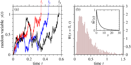
In this paper, we investigate a stochastic inverse problem in the context of another system commonly encountered in biophysics: macromolecule unfolding and molecular adhesion bond rupturing. Macromolecular bond displacements are often described by a single bond coordinate, represented by a fluctuating Brownian “particle” in a one-dimensional energy landscape. The metastable bond is considered to be broken the instant the bond coordinate reaches a critical extension. This problem is of great interest in single-molecule biophysics, particularly in the context of dynamic force spectroscopy (DFS) (Evans et al. 1995). In DFS, a pulling force protocol is applied to the bond and the force at the instant of rupture is recorded. The mean rupture force by itself would give very little information about the molecular potential (Schlierf & Rief 2006) since many different potentials would yield the same mean rupture force. How much of the bond potential can be recovered from the measured rupture force distribution? All of the recent theoretical treatments of this problem have either analysed the forward problem (Heymann & Grübmuller 2000), used physical approximations to derive simple force-dependent and time-dependent dissociation rates (Bell 1978, Walton et al. 2008), and/or considered simple 2-3 parameter single minimum potentials (Hummer & Szabo 2003, Dudko et al. 2008, Freund 2009). The rate of force increase as a function of displacement (the rupture stiffness) has also been incorporated into a procedure to fit basic parameters of simple potentials (Fuhrmann et al. 2008). However, by imposing such simple two or three parameter forms for the reconstructed potential, one loses details such as multiple minima.

Here, we approach the inverse problem by allowing a wider class of potentials, including those with multiple minima. Within a class of potentials, we numerically determine the ones that best fit the entire measured FPTD. Although the difficulty of extracting eigenvalues from FPTD data is avoided, the inverse problem remains intrinsically ill-conditioned and it is not surprising that almost all studies have focused on reconstructing only two or three attributes of the stochastic process, typically, the energy barrier height and width. In §2, we formulate the problem through the backward equation of a Brownian process with a potential energy-derived drift. In §3, we decompose the drift function into basis functions and develop an iterative optimization procedure to find the coefficients of these basis functions. In §4, we show that using a single FPTD restricts the type of potentials we can reconstruct. We also show how the inverse problem can be optimized by tuning the amplitude of the unknown potential and the initial bond displacement. Another key finding is that multiple FPTDs greatly facilitate the reconstruction, allowing us to accurately determine potentials with multiple minima. We propose experimental protocols that can be used to generate these additional FPTDs. Finally in §5, we discuss limitations of our method and possible refinements.

2 Stochastic Theory and the Inverse Problem

The general problem of stochastic bond rupturing is geometrically complex, particularly when considering deformations associated with large macromolecules carrying many degrees of freedom. Although in principle these systems can be modeled by stochastic processes in higher dimensions, for simplicity, and we restrict our mathematical analysis to a one-dimensional Brownian motion described by a diffusivity $D(x)$ and a convective drift $-D(x)(k_{B}T)^{-1}(\mbox{d}\Phi(x)/\mbox{d}x)$ proportional to the force derived from a time-independent molecular bond potential $\Phi(x)$, and to the mobility $D(x)(k_{B}T)^{-1}$. Although we restrict ourselves to time-independent potentials, corresponding to static forces, the rupture force distribution can be transformed into a first rupture time distribution (FPTD) in the quasi-adiabatic limit (Dudko et al. 2008). The continuous Brownian process can be described by the probability $P(y,t|x)\mbox{d}y$ for the bond coordinate to be between positions $y$ and $y+\mbox{d}y$ at time $t$, given that it started at position $x$ at initial time $t=0$. This probability density obeys the backward equation (Gardiner 2004)

$${\partial P(y,t|x)\over\partial t}+{D(x)\over k_{B}T}{\mbox{d}\Phi\over\mbox{d}x}\left({\partial P(y,t|x)\over\partial x}\right)=D(x){\partial^{2}P(y,t|x)\over\partial x^{2}}.$$ (1)

Since the bond is irreversibly ruptured when stretched past a known position $y=L$, we impose the absorbing boundary condition $P(y=L,t|x)=0$. The bond survival probability at time $t$, given that it started initially at position $x$ is found from integrating the probability density over all the final coordinates that an unruptured bond can take, i.e., $S(x,t)=\int_{0}^{L}P(y,t|x)\mbox{d}y$. From $S(x,t)$, we define the FPTD $w(x,t)=-\partial_{t}S(x,t)$, which obeys

$${\partial w(x,t)\over\partial t}+{D(x)\over k_{B}T}{d\Phi(x)\over dx}{\partial w(x,t)\over\partial x}=D(x){\partial^{2}w(x,t)\over\partial x^{2}},$$ (2)

subject to initial condition $w(x,0)=0$, and boundary conditions $\partial_{x}w(x,t)|_{x=0}=0$ and $w(x=L,t)=\delta(t)$.

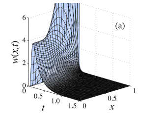
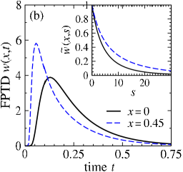
In the forward problem, $\Phi(x)$ and $D(x)$ are given and one solves equation (2) to find the function $w(x,t)$, as shown in figure 2. Each fixed-$x$ slice of the surface $w(x,t)$ represents the FPTD for a particle that started the random walk at position $x$.

Figure 2: (a) The solution to the forward equation 2 for the first passage time distribution (FPTD) as a function of starting position $x$ with $D=1$ , $L=1$ and $U(x)=4-10x+6x^{2}$. The delta function at $t=0$ when $x=1$ was approximated by a sufficiently narrow gaussian centered at $t=0$. (b) For each starting position $x$, slices through the surface define the FPTD $w(x,t)$. Two slices corresponding to the starting positions $x=0$ (solid) and $x=0.45$ (dashed) are shown. Inset: The Laplace transform of the same two slices.

In the inverse problem, the functions $\Phi(x)$ and $D(x)$ are unknown and need to be determined from an experimentally measured or simulated FPTD and a known starting position $x$. In general, the unique pointwise reconstruction of both $D(x)$ and $\Phi(x)$ from FPT data is impossible (Bal & Chou 2003). At best, only half of either $D(x)$ or $\Phi(x)$ can be uniquely determined from a single FPTD (Bal & Chou 2003, Chen et al. 1985). It has been shown that if we assume $D$ is a known constant, then $\Phi(x)$ is uniquely identifiable from a single FPTD provided it is already known over a certain interval within $(0,1]$ (Bal & Chou 2003).

3 Reconstruction Algorithm

Since in this problem, $\Phi(x)$ is not known on any requisite interval, it is not even clear whether $\Phi(x)$ can be uniquely reconstructed. Nevertheless in this section we express $\Phi(x)$ as a superposition of (smooth) basis functions and attempt to reconstruct the coefficients, deferring a rigorous analysis of our algorithm for a future publication. We find that representing $\Phi(x)$ using a relatively small number of basis functions renders the problem computationally tractable, yielding a unique solution in many cases.

Henceforth, we nondimensionalize the problem by measuring distance in units of $L$, time in units of $L^{2}/D$, and the potential $\Phi(x)$ in units of the thermal energy $k_{B}T$. Finally, to avoid numerically representing the $\delta-$function in the boundary condition $w(1,t)=\delta(t)$, we work with the Laplace transform $\tilde{w}(x,s)=\int_{0}^{\infty}w(x,t)e^{-st}\mbox{d}t$, which obeys the infinite set (for each $s\in\mathbb{R}_{\geq 0}$) of uncoupled ODEs

$${\partial^{2}\tilde{w}(x,s)\over\partial x^{2}}+U(x){\partial\tilde{w}(x,s)\over\partial x}=s\tilde{w}(x,s),$$ (3)

subject to the Laplace-transformed boundary conditions $\partial_{x}\tilde{w}(x,s)|_{x=0}=0$ and $\tilde{w}(1,s)=1$.

In equation (3), we have defined the dimensionless drift $U(x)\equiv-\mbox{d}\Phi(x)/\mbox{d}x$. The condition $\partial_{x}\tilde{w}(x,s)|_{x=0}=0$ represents a reflecting boundary at $x=0$ and ensures a nonnegative bond coordinate. Equation (3) is a differential equation in the initial bond position for the Laplace-transformed rupture time distribution $\tilde{w}(x,s)$.

Mathematically, our objective is to reconstruct $U(x)$ and then extract, modulo an irrelevant constant, the unknown potential $\Phi(x)$. However, to do so, we must choose a reduced representation of $U(x)$ that renders, for a chosen value of $x$, and all $s\in\mathbb{R}_{\geq 0}$, $\tilde{w}(x,s)$ as close as possible to the measured or simulated Laplace-transformed FPTD $\tilde{W}(s)$. Since it is known that approximating a function using a basis of monomials leads to a very ill-conditioned problem (Keller 1975), we represent the convection in terms of orthonormal polynomials:

$$U(x)=\sum_{i=0}^{n-1}a_{i}u_{i}(x),$$ (4)

where $\{a_{i}\}\equiv{\bf a}$ is the vector of expansion coefficients, and the first few orthonormal basis functions are

$$u_{0}(x)=1,\,\,u_{1}(x)=\sqrt{3}(1-2x),\,\,u_{2}(x)=\sqrt{5}(1-6x+6x^{2}),\ldots$$ (5)

Our method for reconstructing $U(x)$ consists of using a spectral method (Trefethen 2000) to repeatedly solve the forward problem equation (3) to refine our estimate for the potential.

Starting with an initial guess for the drift (say, $U(x)=0$, the “null” hypothesis), we solve equation (3) for many positive values of $s$ to obtain a numerical approximation for $\tilde{w}(x,s;{\bf a})$. We then compute the “distance” between the $\tilde{w}(x,s;{\bf a})$ and the given data $\tilde{W}(s)$ using the objective function

$$\Pi({\bf a}) = \int_{0}^{\infty}|\tilde{w}(x,s;{\bf a})-\tilde{W}(s)|^{2}g(s)\mbox{d}s,$$ (6)

where $g(s)$ is a function that weights FPT data differently for different $s$. By appropriately adjusting $U(x)$, implemented through small changes in ${\bf a}$, $\Pi({\bf a})$ is decreased. The incremental adjustments in ${\bf a}$ are repeated until $\Pi({\bf a})$ is minimized. Although many different algorithms can be used to minimize $\Pi({\bf a})$, we first consider $g(s)=1$ and choose a safe-guarded Newton strategy that relies essentially on computing the Hessian of $\Pi({\bf a})$. Details of the algorithm are described in 5.

4 Results and Discussion

We test our algorithm and discuss reconstructing the drift function $U(x)$ from (i) a single, perfectly measured distribution of rupturing times, and (ii) multiple perfectly measured distributions of rupturing times, realized under different experimental conditions. We first generate perfect “data” by solving the forward problem using a hypothetical target potential function $\Phi^{*}(x)$ (and corresponding $U^{*}(x)=\sum_{i=0}^{n-1}a_{i}^{*}u_{i}(x)$). After generating the data $\tilde{W}(s)=\tilde{w}(x,s;{\bf a}^{*})$, we pretend we did not know the coefficients ${\bf a}^{*}$, and try to reconstruct them by minimizing $\Pi({\bf a})$ through successive iterations $k$ of the numerical algorithm detailed in 5. Starting from an initial guess for ${\bf a}(k=0)={\bf 0}$, we investigate if and how ${\bf a}(k)$ approaches ${\bf a}^{*}$, and the number of coefficients $a_{i}$ that can be reliably reconstructed. Using a single FPTD, we find that reconstruction of $\Phi^{*}(x)$ is badly conditioned for $n\gtrsim 4$, but that using two or more distinct FPTDs allows us to easily find 5 or more coefficients of $\Phi^{*}(x)$ in many cases.

4.1 Single measurement

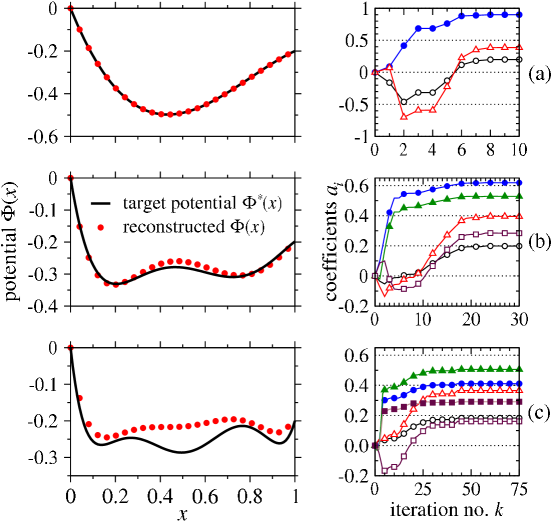
We first assume a target potential $\Phi^{*}(x)=-({1+7\sqrt{3}\over 5})x+{12\sqrt{3}\over 5}x^{2}-\sqrt{3}x^{3}$ corresponding to a target drift function $U^{*}(x)$ parametrized by $(a_{0}^{*},a_{1}^{*},a_{2}^{*})=({1\over 5},{9\over 10},\sqrt{{3\over 20}})$. Figure 3(a) shows that starting with the initial guess $U(x)=0$, minimizing the objective function equation (6) leads to accurate convergence to the unknown target drift $U^{*}(x)$ within $\sim 10$ iterations. We find in figure 3(b) that a five-parameter potential is typically a marginal case in that it can only be occasionally reconstructed, and only after a large number of iterations. However, we are typically not able to accurately reconstruct a potential with six parameters (see figure 3(c)), regardless of the number of iterations.

Figure 3: Reconstruction of three, five and six parameter potentials. Row (a): reconstruction of a three parameter potential corresponding to drift coefficients $(a^{*}_{0},a^{*}_{1},a^{*}_{2})=(1/5,9/10,\sqrt{3/20})$. Row (b): attempted reconstruction of a five parameter double-well potential with coefficients $\mathbf{a}^{*}=(1/5,3/5,2/5,3/5,\sqrt{2}/5)$. Row (c): failed reconstruction of a six-parameter potential defined by ${\bf a}^{*}=(1/5,1/2,2/5,1/2,1/5,\sqrt{13/50})$. In the second column, the coefficient values $a_{0},a_{1},a_{2},a_{3},a_{4},a_{5}$ at each iteration are indicated by open circles, filled circles, open triangles, filled triangles, open squares, and filled squares, respectively.

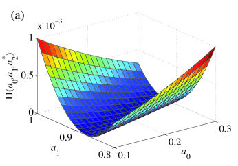
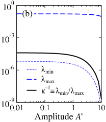
When the unknown target drift function $U^{*}(x)$ is structurally more complex, extremely slow or nonconvergence to ${\bf a}^{*}$ arises because the curvature of $\Pi({\bf a})$ near the true minimum, in at least one direction, becomes extremely small. Since our minimization algorithm relies on essentially inverting the $n\times n$ Hessian matrix $H_{ij}=\partial_{a_{i}}\partial_{a_{j}}\Pi|_{{\bf a}={\bf a}^{*}}$ (see 5), the mathematical feasibility of the reconstruction is limited by its condition number $\kappa\equiv\lambda_{\rm max}/\lambda_{\rm min}$. Here, $\lambda_{\rm max}$ and $\lambda_{\rm min}$ are the largest and smallest eigenvalues of $H$, representing the largest and smallest curvatures of $\Pi({\bf a})$ at ${\bf a}^{*}$, along the corresponding eigendirections, respectively. In addition to increasing the number of eigendirections, increasing $n$ rapidly decreases, in particular, the minimum curvature $\lambda_{\rm min}$, thereby increasing $\kappa\equiv\lambda_{\rm max}/\lambda_{\rm min}$ and making the minimum in $\Pi({\bf a})$ harder to find. As shown in .3, larger values of $i$ and $j$ correspond to more rapidly oscillating basis functions that reduce the magnitude of $H_{ij}$. This property renders the problem badly conditioned and is the underlying mathematical reason for the difficulty of extracting more than three parameters from a given potential landscape. To explicitly illustrate the ill-conditioning of the problem, we plot in figure 4(a) the three-parameter objective function $\Pi(a_{0},a_{1},a_{2}^{*})$ (with $g(s)=1$) as a function of the parameters $a_{0}$ and $a_{1}$. Although the global minimum in $\Pi({\bf a})$ occurs at $(a_{0}^{*},a_{1}^{*})$, it is clear that the curvature near the minimum is extremely small along at least one direction, making the minimum difficult to find numerically.

Figure 4: (a) Objective function $\Pi(a_{0},a_{1},a_{2}^{*})\equiv\int_{0}^{\infty}|\tilde{w}(x=0.3,s;a_{0},a_{1},a_{2}^{*})-\tilde{w}(0.3,s;a_{i}^{*})|^{2}\mbox{d}s$ for the potential shown in Fig 2(a) as function of $a_{0}$ and $a_{1}$. Projected onto $a_{0}-a_{1}$ space, $\Pi$ exhibits a much smaller curvature in one direction compared to the orthogonal direction. (b) The minimum and maximum curvatures of $\Pi({\bf a})$, and the inverse condition number. For constant weighting $g(s)$ defined in equation (6), we find that the condition number $\kappa$ decreases monotonically as the amplitude of the target potential $A^{*}\rightarrow 0$.

Since all three target potentials considered in figure 3 were chosen to have $|{\bf a}^{*}|^{2}=1$, figure 3 fairly compares the reconstruction of different-shaped potential functions with equal amplitude While increasing the dimension $n$ makes the problem more ill-conditioned, for fixed $n$, reconstruction efficiency may nonetheless depend on the typical magnitude of the potential to be reconstructed. To compare reconstructions of potentials of different expected magnitudes, we define the amplitude factor

$$A^{*}\equiv\sqrt{\sum_{i=0}^{n-1}(a_{i}^{*})^{2}}=|{\bf a}^{*}|$$ (7)

for each target drift function. While the amplitude $A^{*}$ needs to be found from reconstructing the values of $a_{i}^{*}$, its value sets the scale of the unknown drift function relative to thermal diffusion and defines an effective Peclet number for this problem. Experimentally, the shapes of potentials are fixed by molecular details; however, the Peclet number $A^{*}$ is inversely proportional to temperature and can in principle be tuned experimentally.

Figure 4(b) shows that for a fixed-shape target drift function $U^{*}(x)$ of the form ${\bf a}^{*}=A^{*}\times(1/5,9/10,\sqrt{3/20})$, and a single a FPTD measurement, the inverse of the condition number is maximized in the limit $A^{*}\rightarrow 0$. Therefore, the problem has the best conditioning and the most efficient mathematical reconstruction in the zero Peclet number limit, when the potentials are weak. Computationally, a single FPTD data set arising from a vanishingly small drift perturbing the purely diffusive problem gives the most numerical “signal” for reconstructing the coefficients of $U^{*}(x)$. Although the magnitudes of $a_{i}$ are vanishingly small, their incremental effect on reducing the condition number $\kappa$ is nonetheless greatest in this limit. This optimal limit arises from a mathematical analysis and is not predicted by physical considerations. However, system and experimental constraints may preclude measurement of effective potentials at extremely low Peclet numbers $A^{*}$ (high temperatures), suggesting that an optimal, intermediate temperature may still arise in practice.

Figure 5: Inverse condition number as a function of starting position $x$ and drift amplitude (Peclet number) $A^{*}$ for three different potentials. (a) $\Phi^{*}(x)=-A^{*}{\sqrt{3}\over 2}x^{2}$ (b) $\Phi^{*}(x)=A^{*}\left[-{3\sqrt{3}\over 7}x+{2\sqrt{3}\over 7}x^{2}\right]$ (c) $\Phi^{*}(x)=A^{*}\left[-({1+7\sqrt{3}\over 5})x+{12\sqrt{3}\over 5}x^{2}-\sqrt{3}x^{3}\right]$. The ratio $\kappa^{-1}=\lambda_{\rm min}/\lambda_{\rm max}$ is typically maximal for $A^{*}\rightarrow 0$ and $x\sim 0.75$.

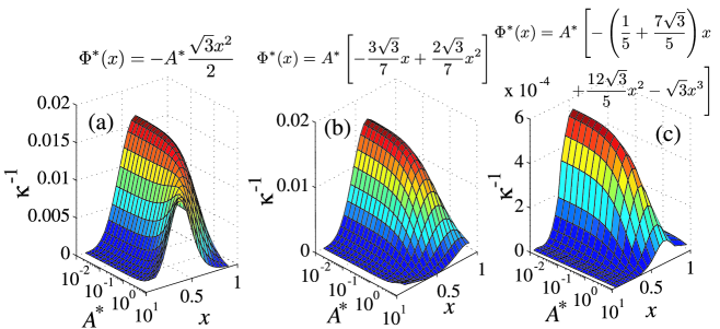
In figure 5, the behavior of $\kappa^{-1}$ as a function of starting position is even more intriguing. For constant $g(s)$ and all potentials we tested, the optimal value of the starting position occurs roughly near $x=0.7-0.9$. This starting position is close to the rupture point at $x=1$ and is somewhat insensitive to the amplitude $A^{*}$, except for very large $A^{*}$. The robustness of this optimal starting position arises from analysing the Hessian matrix, in particular the dependence of its condition number on $x$.

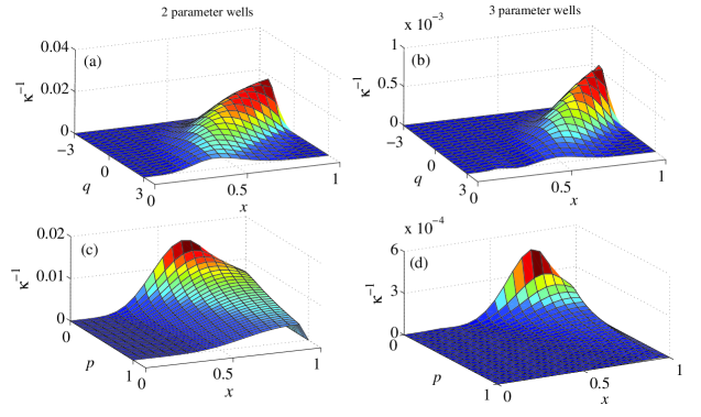
From the form of $H_{ij}$ (see equation (19)), we can show numerically that $\lambda_{\rm min}$ has a maximum for $x\approx 0.7-0.9$ and that the behavior of $\kappa^{-1}$ is rather insensitive to changes in $\lambda_{\rm max}$; thus, $\kappa^{-1}$ is typically maximal near $x=0.75$. For the three qualitatively different potentials used in figure 5, the optimal starting positions all fall approximately within $x=0.7-0.9$ for a wide range of amplitudes $A^{*}$. In these examples, the best conditioning occurs in the limit $A^{*}\rightarrow 0$, consistent with figure 4(b). For nonconstant $g(s)$, the approximate optimal starting position $x$ typically ranges from 0.5 to 0.9, depending on the form of $g(s)$ (cf. figure 7 in .3).

4.2 Multiple measurements

Since a single measurement $\tilde{W}(s)$ is typically insufficient to reconstruct the potential well beyond three coefficients, even after optimizations with respect to Peclet number $A^{*}$ and starting position $x$, we consider how additional data can be used to refine the reconstruction of $U^{*}(x)$. As indirectly suggested by the analysis of varying $A^{*}$ and $x$, an unknown potential can be changed by a specified amount to yield a FPTD different from that of the original unchanged potential. By imposing any number of perturbations, multiple FPTD data $\tilde{W}$ can be measured and used to aid the reconstruction of the original potential.

We propose three protocols for modifying the potential to be reconstructed. Experimentally, these protocols correspond to changing the system temperature, applying then quickly removing a force to change the starting position, and adding an applied force at the start of the stochastic process. Mathematically, these perturbations correspond to specific changes in $A^{*}$, $x$, and the form of the potential $\Phi^{*}$, respectively. The multiple FPT distributions, measured under different conditions, can then be combined into a multi-distribution objective function. We summarize the protocols below:

$\bullet$ Changing amplitude via temperature - One way to obtain additional data is by changing the amplitude (or effective Peclet number) $A^{*}$ of the unknown drift. For each distinct value of $A^{*}$, a separate FPTD $\tilde{w}(x,s;{\bf a}^{*})$ can be measured. These different FPTD’s all arise from bond potentials with the same underlying shape, and can be used together to better reconstruct $\Phi^{*}(x)$. While the absolute value of $A^{*}$ needs to be determined from the reconstruction of ${\bf a}^{*}$, the relative temperature at which a second measurement is taken can be used to determine the ratio $\theta_{2}^{*}\equiv A_{2}^{*}/A_{1}^{*}$.

$\bullet$ Tuning starting positions - By adding a force to the system before the start of the process, one can adjust the initial position $x$ of the bond. At $t=0$, this force is released, and the stochastic process proceeds under the original target drift $U^{*}(x)$, provided the potential relaxes quickly to $\Phi^{*}(x)$. Stochastic bond dynamics starting at different positions $x$ yield different measured FPT distributions.

$\bullet$ Adding Probe Forces - Finally, one can add known potentials to the original target potential immediately after the start of the stochastic process to obtain additional FPT distribution data. Here, $\Phi^{*}(x)\rightarrow\Phi^{*}(x)+\Delta\Phi(x)$, where $\Delta\Phi(x)$ is known. The associated drift then changes according to $U^{*}(x)\rightarrow U^{*}(x)+\Delta U(x)$, where $\Delta U(x)$ is implemented through a known change in the expansion coefficients $\Delta{\bf a}$ and represents an externally applied force imposed by e.g., a pulling device such as an AFM tip or an optical tweezer. The associated external potential in such cases may be of the form $\Delta\Phi(x)=-F_{\rm ext}x-Kx^{2}/2$, where $F_{\rm ext}$ is the externally applied time-independent force and $K$ is the elastic response of the pulling device. In this case, the new total bond potential $\Phi^{*}+\Delta\Phi(x)$ induces a drift $U^{*}(x)+\Delta U$ defined by ${\bf a}^{*}+\Delta{\bf a}$ where $\Delta a_{0}=F_{\rm ext}+K/2$ and $\Delta a_{1}=-K/(2\sqrt{3})$. This new drift gives rise to another, different FPTD.

An objective function that incorporates all $M$ FPT distributions measured under $M$ different conditions described above can be defined as

$$\Pi_{M}({\bf a})=\sum_{m=1}^{M}\int_{0}^{\infty}[\tilde{w}(x_{m},s;\theta_{m}^{*},{\bf a}+\Delta{\bf a}_{m})-\tilde{W}(s)]^{2}g_{m}(s)\mbox{d}s,$$ (8)

where $x_{m}$, $\Delta{\bf a}_{m}$, and $\theta_{m}^{*}\equiv A^{*}_{m}/A_{1}^{*}$ denote the known starting position, added pulling force, and relative temperature of the $m^{\rm th}$ measurement, respectively. The function $g_{m}(s)$ weights each of the $m$ measurements differently. If the data $\tilde{W}$ in equation (8) were generated from a target drift $U^{*}(x)$, as is the case in our analyses, then it is defined as $\tilde{W}(s)\equiv\tilde{w}(x_{m},s;\theta_{m}^{*},{\bf a}^{*}+\Delta{\bf a}_{m})$. Measured data $\tilde{W}$ should be obtained with different starting position $x_{m}$, applied force $\Delta{\bf a}$, and/or different temperature ratios $\theta_{m}^{*}$ with at least one of the known parameters $x_{m},\Delta{\bf a}_{m},A^{*}_{m}$ different among the $M$ measurements. Multiple data sets provide additional constraints, increasing the curvature of the objective function near ${\bf a}^{*}$. In general, the smallest eigenvalue $\lambda_{\rm min}$ of the Hessian matrix associated with $\Pi_{M}$ increases with $M$. Upon minimizing the multi-FPTD objective function $\Pi_{M}$, we obtain ${\bf a}^{*}$.

Figure 6: Attempted reconstruction of 5-parameter potential wells (solid black) using single and double data sets. (a) Blue dotted and red dashed lines: reconstructions from single data sets generated using $A^{*}_{1}=6.11755\ldots$ and $A^{*}_{2}=A^{*}_{1}/5$ respectively. Circles: reconstruction using both data sets. Original potential was parametrized by ${\bf a}^{*}=(-1/10,11\sqrt{3}/5,89/(14\sqrt{5}),8/\sqrt{7},50/21)$, starting position was $x=0.170$. (b) Blue dotted and red dashed lines: reconstructions from single data sets generated using $x_{1}=0.182$ and $x_{2}=0.727$ respectively. Circles: reconstruction using both data sets. Original potential was parametrized by ${\bf a}^{*}=(2/3,2,5/3,2,4/3)/\sqrt{13})$, starting position was $x=0.170$. (c) Blue dotted and red dashed lines: reconstructions from single data sets generated without and with probe force $\Delta U=x$. Circles: reconstruction using both data sets $\Delta U=0$ and $\Delta U=x$. Target potential was parametrized by ${\bf a}^{*}=(2/3,2,5/3,2,4/3)/\sqrt{13})$, starting position was $x=0.642$.

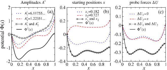
To illustrate how additional data can improve potential reconstruction, we compare how including two FPT distributions ($M=2$) in our objective function $\Pi$ simultaneously affects reconstruction relative to using each FPTD separately. The two distributions will arise from two ideal measurements taken under two different conditions within each of the proposed experimental protocols described above. In Figure 6(a), we attempt to reconstruct the five-parameter, double-well potential $\Phi^{*}(x)=-28x+\frac{1451}{10}x^{2}-307x^{3}+290x^{4}-100x^{5}$ using two “temperatures.” This potential corresponds to $A^{*}_{1}=|{\bf a}^{*}|=6.11755\ldots$. We then generated data associated with $\Phi^{*}(x)/5$, corresponding to $A_{2}^{*}=A_{1}^{*}/5=1.22351\ldots$. Reconstruction of the original $\Phi^{*}(x)$ using each individual FPTD fails, as does using both FPTD data sets. In figure 6(b), we see that while using data sets corresponding to either initial position $x_{1}=0.182$ or $x_{2}=0.727$, the algorithm fails to reconstruct the target potential. However, using both initial positions together allows us to accurately determine $\Phi^{*}(x)$. Similarly, adding the perturbing potential $\Delta\Phi_{2}=-x^{2}/2$ ($\Delta U_{2}=x$) provides another FPTD that allows accurate reconstruction of a double-well potential (figure 6(c)).

5 Summary and Conclusions

We have analysed the mathematical aspects of reconstructing the drift of a stochastic process from perfectly measured first passage time distributions. In practice, insufficient number of bond rupture events are currently measured to enable quantitative potential reconstruction; therefore, we used numerically generated data to illustrate our main mathematical results. For single distributions, only very coarse attributes (approximately three parameters) can be reconstructed. We demonstrate how to optimize the efficiency of the reconstruction by controlling the effective amplitude or Peclet number $A^{*}$ and starting position $x$ of the stochastic process. If only one FPTD can be measured, our analysis suggests that $A^{*}\rightarrow 0$ and $x\sim 0.75$ are the most likely parameters to give the best chance for reconstructing relatively simple potentials. However, these findings were found numerically by assuming perfect data, uniform diffusivity, precisely defined starting positions $x$, and a constant weighting function $g(s)$. In practice, finite time resolution, noisy data, and other experimental limitations may be accounted for by a more suitable weighting function $g(s)$ (or $g(t)$ if $\Pi$ were a functional of $w(x,t)$ and the data $W(x,t)$). We show in .3 that the optimal parameters $A^{*}$ and $x$ can change when a nonconstant weighting function $g(s)$ is used. While the optimal values of $A^{*}\rightarrow 0$ and $x\sim 0.75$ (for $g(s)=1$) were found numerically, without physically realistic limitations, they nonetheless provide a possible experimental starting point.

We also showed that additional measurements in the form of multiple FPTDs can be used to provide dramatically better conditioning of the problem, allowing finer details of the drift function to be extracted. The total objective function including the constraints from all $M$ measurements has a sharper minimum, increasing the efficiency of standard optimization algorithms. We proposed three ways of obtaining additional measurements under different experimental conditions: tuning the effective amplitude or Peclet number $A^{*}$ through the system temperature, adjusting the starting position $x$ via an initially applied force, and adding a known “probe” force through a potential $\Delta\Phi$. This later potential can be realized in a number of ways, from directly mechanically pulling on the bond, to using mutagenesis to systematically change local properties of the bond energy profile. Such mutant bonds may provide additional FPTD data facilitating reconstruction of the original “wild-type” potential.

A number of refinements are suggested by our analysis, and some are discussed in the Appendices. For example, rather than Laplace-transforming the data, one can directly fit to $W(x,t)$. Although this approach is computationally more expensive, it would allow us to treat time-dependent potentials $U(x,t)$, and directly analyze dynamic force spectroscopy experiments (Evans et al. 1995, Heymann & Grubmüller 2000, Fuhrmann et al. 2008), or scenarios in which the temperature is changed in a time-dependent way (Getfert & Reimann 2009). Moreover, specific to the bond rupture problem, data involving bond coordinates as a function of time, if accurately measured, can also be incorporated into the objective function. These additional data may be useful in combating the noise problem and help improve the overall conditioning.

Other more mathematical refinements and extensions can also be implemented, including exploring effects of using different basis functions for $U(x)$, using more sophisticated optimization methods, quantifying the reconstruction efficiency for large $M$, defining the experimentally-imposed weighting function $g(s)$, reconstruction of the diffusivity $D(x)$ itself, and systematically exploring the effects of noise in the data. Here, a Bayesian approach to estimate likelihood functions for the coefficients ${\bf a}^{*}$, or information criteria to choose the size $n$ of the basis expansion might be useful (Getfert et al. 2009).

Numerical Methods

.1 Numerical scheme for solution of the Backward Equation

In the forward problem, with $D(x)$ and $\Phi(x)$ given, equation (2) can be solved using standard finite difference schemes. Figure 2(b) shows numerically computed FPTDs for two different starting positions with $D=L=1$, $U(x)=4-10x+6x^{2}$. The singular boundary condition $w(x=1,t)=\delta(t)$ is treated by taking Laplace transforms in time of equation (2) and solving equation (3) for all values of the Laplace-transform variable $s$. Moreover, the numerical solution of equation (3) for a set of values $s$ can be found much more quickly than solving the full partial differential equation on a large $x-t$ grid. For $D=1$ and a given drift function $U(x)$, we use a spectral method (Trefethen 2000) to solve the Laplace-transformed Backward Equation (3). First, the spatial domain is mapped from $[0,1]$ to $[-1,1]$ using a change of variable. Then, the function $\tilde{w}(x,s)$ is represented by $\tilde{w}(x_{i},s)\equiv\tilde{w}_{i}$ and interpolated between the $N$ Chebyshev points $x_{i}=\cos\left({(i-1)\pi\over N-1}\right)$ with polynomials. The resulting $N\times N$ system of equations for $\tilde{w}_{i}$ are

$$Q_{ij}\tilde{w}_{j}=\delta_{1,i},$$ (9)

where the matrix $Q_{ij}$ is

$$\begin{array}[]{rcl}Q_{1j}&=&\delta_{1j},\\ Q_{ij}&=&4({\bf D}_{N}^{2})_{ij}+2({\bf U}{\bf D}_{N})_{ij}-s\delta_{ij},\quad i=2,...,N-1,\quad j=1,2,...,N\\ Q_{Nj}&=&({\bf D}_{N})_{Nj},\quad j=1,2,...,N,\end{array}$$ (10)

where ${\bf D}_{N}$ is the usual $N\times N$ pseudospectral differentiation matrix (Trefethen 2000) and the diagonal matrix $\mathbf{U}$ is defined by

$$U_{ij}=U(x_{i})\delta_{ij}.$$ (11)

We used $N=51$ spectral points in all of our computations within the iterative algorithm. Fixed$-x$ slices of the numerically obtained functions $\tilde{w}(x,s)$ are qualitatively similar to the plots shown in the inset of figure 2(b).

.2 Evaluation of the objective function

In our analysis, we generate data by numerically computing distributions derived from a target drift function $U^{*}(x)$ (defined by its polynomial coefficients ${\bf a}^{*}$). Since the data is generated numerically, we use $\tilde{W}(x,s)\equiv\tilde{w}(x,s;{\bf a}^{*})$ in the objective function and write

$$\Pi(\mathbf{a})=\int_{0}^{\infty}[\tilde{w}(x,s;\mathbf{a})-\tilde{w}(x,s;\mathbf{a}^{*})]^{2}g(s)\mbox{d}s.$$ (12)

Note that the $\ell^{\rm th}$ moment of the FPTD is given by

$$\langle T^{\ell}\rangle=(-1)^{\ell}{\partial^{\ell}\tilde{w}(x,s)\over\partial s^{\ell}}\bigg{|}_{s=0}.$$ (13)

Therefore for two FPTDs with identical first few moments, their first few derivative are also identical. Such FPTDs can be distinguished only their difference at larger values of $s$ (and the function $g(s)$ in equation (12) can be used to weight these differences accordingly). Only information contained in the tails of the Laplace-transformed distributions can distinguish two FPT distributions with equal lower moments. Therefore for the algorithm described in 5 to be effective, a numerical approximation to the integral in equation (12) must evaluate the integrand for sufficiently large values of $s$. This can be done by mapping $s\in[0,\infty]$ to $\xi\in[0,1]$ through a change in variable $s(\xi)=\xi/(1-\xi)$, and computing

$$\Pi(\mathbf{a})=\int_{0}^{1}[\tilde{w}(s(\xi);{\bf a})-\tilde{w}(s(\xi);\mathbf{a}^{*})]^{2}g(s(\xi))\frac{\mbox{d}\xi}{(1-\xi)^{2}}.$$ (14)

In order to choose $g(s)$ such that $\Pi({\bf a})$ remains convergent, we assume that $g(s)$ has no singularities in $s\in\left(0,\infty\right)$ and consider the behavior of the integrand at the end points $s=0$ and $s=\infty$ through the asymptotic expansions

$$\begin{array}[]{rcl}\tilde{w}(s)&=&\int_{0}^{\infty}e^{-st}w(t)\mbox{d}t\\ &\sim&\displaystyle\sum_{n=0}^{\infty}\frac{w^{(n)}(0)n!}{s^{n+1}},\qquad s\gg 1,\end{array}$$ (15)

and

$$\tilde{w}(s)\sim\sum_{n=0}^{\infty}\frac{s^{n}\tilde{w}^{(n)}(0)}{n!},\qquad s\ll 1.$$ (16)

Since $w(t=0;{\bf a})=w(t=0;{\bf a}^{*})=0$ for any two sets of drift coefficients $\mathbf{a}$ and $\mathbf{a^{*}}$, the asymptotic expansion (15) implies that $[\tilde{w}(s;{\bf a})-\tilde{w}(s;{\bf a}^{*})]^{2}=O(s^{-4})$ as $s\to\infty$. If the first $k$ time derivatives of $w(t;{\bf a})$ and $w(t;{\bf a}^{*})$ match, equation (15) implies that $[\tilde{w}(s;{\bf a})-\tilde{w}(s;{\bf a}^{*})]^{2}=O(s^{-2(k+2)})$. For a weighting function of the form $g(s)=s^{q}$, the integrand in equation (14) is $O((1-\xi)^{2-q})$ as $\xi\to 1$ and is integrable at $\xi=1$ provided $q<3$.

Since $\tilde{w}(s=0;{\bf a})=\tilde{w}(s=0;{\bf a}^{*})=1$, the asymptotic expansion (16) implies that $[\tilde{w}(s;{\bf a})-\tilde{w}(s;{\bf a}^{*})]^{2}=O(s^{2})$ as $s\to 0$. If the first $k$ $s$-derivatives agree (i.e. the first $k$ moments of $w(t;{\bf a})$ and $w(t;{\bf a}^{*})$ are identical), equation (16) implies that $[\tilde{w}(s;{\bf a})-\tilde{w}(s;{\bf a}^{*})]^{2}=O(s^{2(k+1)})$. If $g(s)=s^{q}$ then the integrand in equation (14) is $O(\xi^{2+q})$ as $\xi\to 0$ and is integrable at $\xi=0$ provided $q>-3$.

To summarize, if we take $A(s)=s^{q}$, then convergence of the integral in equation (14) requires $-3<q<3$. When evaluating $\Pi({\bf a})$, a fourth order open trapezoid rule (that does not require evaluation of the integrand at the end points) was used and typically 100-1000 uniformly spaced trapezia were found to give sufficient accuracy for the plots shown in Figs. 3 and 6.

.3 Minimization of $\Pi({\bf a})$

The linear system (3) must be solved for many different values of $s$ so that it can be used in the discrete approximation to the objective function (6). To minimize (6), we use a safe-guarded Newton strategy:

$${\bf a}(k+1)={\bf a}(k)-\sigma{\bf G}^{-1}({\bf a}(k))\nabla_{\bf a}\Pi({\bf a}(k)).$$ (17)

Here, ${\bf G}$ is a positive definite matrix and $\sigma>0$ is the step size chosen to minimize $\Pi({\bf a}(k+1))$ along the descent direction ${\bf G}^{-1}\nabla_{\bf a}\Pi$.

To compute ${\bf G}$, we adopt the following procedure. If the Hessian $H_{ij}\equiv\partial_{a_{i}}\partial_{a_{j}}\Pi({\bf a})$ is positive definite, we set ${\bf G}\equiv{\bf H}$. If the Hessian ${\bf H}$ is not positive definite, we choose a small Tikhonov regularization (Vogel 2002) parameter $\alpha$ such that ${\bf H}+\alpha{\bf I}$ is safely positive definite (${\bf I}$ is the identity matrix) and set ${\bf G}={\bf H}+\alpha{\bf I}$. In either case, ${\bf G}^{-1}$ is also positive definite and moving in the direction of $-\sigma{\bf G}^{-1}\nabla_{a}\Pi$ is guaranteed to decrease $\Pi({\bf a}(k+1))$ for sufficiently small $\sigma$. The value of $\sigma$ is found by performing an exact line search to minimize $\Pi({\bf a}(k+1))$ along the descent direction. All Jacobian and Hessian matrices are approximated numerically using a suitably small $\delta{\bf a}$, typically on the order of $10^{-5}$. The algorithm terminates when the relative change in the objective function is less than $10^{-3}$.

We represent the drift function $U(x)$ using orthonormal polynomials on $[0,1]$ given in equation (5). Often, the potential and drift arising from molecular interactions diverge as $x\rightarrow 0$ (such as in the Lennard-Jones potential). In this case, $\Phi(x)$ and $U(x)$ could be represented using basis functions with the correct divergent behavior for $x\to 0$. Although the Laplace-transformed backward equation (3) has an irregular singular point in this case, the spectral method retains its ability to find solutions as long as $x=1$ is removed from Chebyshev grid.

Analysis of Eigenvalues and Condition Numbers

Since the ease of minimizing $\Pi({\bf a})$ is quantified by the condition number $\kappa\equiv\lambda_{\textrm{max}}/\lambda_{\textrm{min}}$ of the Hessian ${\bf H}$, we now consider the behavior of the minimum and maximum eigenvalues $\lambda_{\rm min}$ and $\lambda_{\rm max}$. If $\kappa=O(1)$, the problem is well-conditioned; if $\kappa\gg 1$, the problem is badly conditioned. Clearly, the one parameter optimization problem has $\kappa\equiv 1$ and is well-conditioned. However, when the number of parameters increases, it is desirable to find conditions under which $\kappa^{-1}$ is maximized.

Figure 7: Inverse condition number $\kappa^{-1}$ in the $A^{*}\rightarrow 0$ limit as a function of starting position $x$ and the weighting function $g(s)$ used in the objective function $\Pi({\bf a})$. In this limit all potentials (with a fixed number of parameters) have the same Hessian. (a) Two parameter potentials with weighting function $g(s)=s^{q}$. (b) Three parameter potentials with weighting function $g(s)=s^{q}$. (c) Two parameter potentials with weighting function $g(s)=e^{-ps}$. (d) Three parameter potentials with weighting function $g(s)=e^{-ps}$.

.4 Small Peclet number analysis

We now analyze $\kappa$ in the $A^{*}\ll 1$ limit. The components of the Hessian at $\mathbf{a}^{*}$ (the drift coefficients of the target potential) are given by

$$H_{ij}=\left.\frac{\partial^{2}\Pi({\bf a})}{\partial a_{i}\partial a_{j}}\right|_{\mathbf{a}=\mathbf{a}^{*}}=2\int_{0}^{\infty}\left.g(s)\left(\frac{\partial{\tilde{w}}}{\partial{a_{i}}}\frac{\partial{\tilde{w}}}{\partial{a_{j}}}\right)\right|_{\mathbf{a}=\mathbf{a}^{*}}\mbox{d}s.$$ (18)

For weak potentials, we find solutions to $\tilde{w}^{\prime\prime}+U(x)\tilde{w}^{\prime}=s\tilde{w}$ in the $U(x)\rightarrow 0$ limit. If $U(x)=O(A^{*})$, we expand the solution in the form $\tilde{w}(x,s)=\sum_{m=0}^{\infty}\tilde{w}_{m}(x,s)$ where $\tilde{w}_{m}=O({A^{*}}^{m})$, and use the boundary conditions $\tilde{w}_{0}(1,s)=1$, $\tilde{w}^{\prime}_{0}(0,s)=0$ and $\tilde{w}_{m}(1,s)=\tilde{w}^{\prime}_{m}(0,s)=0$ ($m\geq 1$) where primes denote differentiation with respect to $x$. The first two terms in the expansion are

$$\tilde{w}_{0}(x,s) = \frac{\cosh\sqrt{s}x}{\cosh\sqrt{s}},$$

$$\tilde{w}_{1}(x,s) = \frac{\sqrt{s}}{\cosh\sqrt{s}}\int_{0}^{1}G(x,x^{\prime})U(x^{\prime})\sinh\sqrt{s}x^{\prime}\mbox{d}x^{\prime},$$

where the Green’s function

$$G(x,x^{\prime})={\sinh\sqrt{s}(1-x_{>})\cosh\sqrt{s}x_{<}\over\sqrt{s}\cosh\sqrt{s}},$$

satisfies $G^{\prime\prime}-sG=-\delta(x-x^{\prime})$ and $x_{<}(x_{>})$ is the lesser(greater) value of $x,x^{\prime}$. Upon using the full orthonormal polynomial expansion $U(x)=\sum_{i=0}^{\infty}a_{i}u_{i}(x)$, we find explicitly

$$H_{ij}=\int_{0}^{\infty}\!\frac{2g(s)s}{\cosh^{2}\sqrt{s}}~{}\mbox{d}s\int_{0}^{1}\!\int_{0}^{1}\!G(x,y)G(x,y^{\prime})u_{i}(y)u_{j}(y^{\prime})\sinh(\sqrt{s}y)\sinh(\sqrt{s}y^{\prime})\mbox{d}y\mbox{d}y^{\prime}.$$ (19)

Since all elements of ${\bf H}$ are independent of the drift coefficients $a_{i}$, they are also independent of $A^{*}$, and so are all eigenvalues. Therefore, as a function of $A^{*}$, the inverse condition number $1/\kappa\equiv\lambda_{\textrm{min}}/\lambda_{\textrm{max}}$ approaches a constant as $A^{*}\rightarrow 0$. Moreover, for all forms of $g(s)$ tested, we find numerically that $\kappa^{-1}$ is maximal in the $A^{*}\rightarrow 0$ limit. These results confirm the numerical data in figure 4(b) and figure 5.

Within the $A^{*}\rightarrow 0$ limit, different weightings $g(s)$ can also be used to better maximize $\kappa^{-1}$. Using the asymptotic form (19) for the Hessian and $g(s)=s^{q}$ ($-3<q<3$), we plot $\kappa^{-1}$ as a function of starting position $x$ and exponent $q$ in Fig 7. Note that $q>0$ puts more weight into the tails of $[\tilde{w}(x,s;\mathbf{a})-\tilde{w}(x,s;\mathbf{a}^{*})]^{2}$, accentuating differences in higher moments of the FPTD. If $q<0$, more weight is given to small values of $s$. For each value of $q$, there is an optimal starting position $x^{*}$ that minimizes the condition number and greatly improves the efficiency of reconstructing the bond potential. Although in §4 we discussed changing the starting positions to optimize the reconstruction, in cases where the starting position cannot be controlled, another strategy may be to estimate an optimal $q=q^{*}$ from figure 7 and minimize $\Pi({\bf a})$ using the weighting function $g(s)=s^{q^{*}}$. We also experimented with weighting functions of the form $g(s)=e^{-ps}$ for $p>0$: see figure 7(c) and 7(d). This class of weighting functions seems to give poorer conditioning compared to $g(s)=s^{q}$ since $\kappa^{-1}$ is generally smaller.

.5 Conditioning with multiple data sets

Figure 8: The inverse condition number $\kappa^{-1}$ as a function of the potential’s magnitude $A^{*}$ for one and two data sets. The thin solid curve corresponds to one FPTD ($M=1$), while broken curves correspond two FPTDs ($M=2$) obtained under different conditions. The dotted curve represents $\kappa^{-1}$ when $A^{*}$ and $A^{*}/5$ are used in the multi-distribution objective function $\Pi_{M}({\bf a})$ (see equation (8)). The dot-dashed curve corresponds to $\kappa^{-1}$ when $x_{1}=0.433$ and $x_{2}=0.65$. Finally, the long dashed curve represents the inverse condition number when two target drifts $U^{*}(x)$ and $U^{*}(x)+5x$ are used. The weighting functions $g_{m}(s)=1$ in all computations.

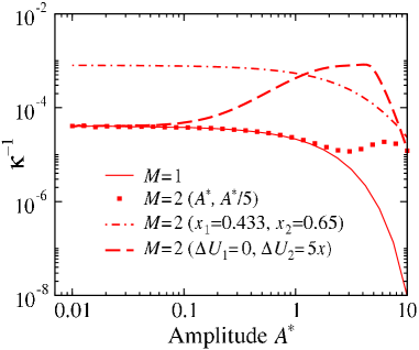
In figure 8, we assumed $g(s)=1$ and plot the inverse condition number $\kappa^{-1}=\lambda_{\rm min}/\lambda_{\rm max}$ as a function of the Peclet number $A^{*}$. The potential used was proportional to the one in figure 3(a): $\Phi^{*}(x)=A^{*}\left[-({1+7\sqrt{3}\over 5})x+{12\sqrt{3}\over 5}x^{2}-\sqrt{3}x^{3}\right]$. The starting position was $x=0.433$. The thin solid curve in figure 8 is taken from figure 4(b) and corresponds to $\kappa^{-1}$ when only one FPTD data set ($M=1$) is used. We compare these values to those when two FPTDs ($M=2$) are used as data in $\Pi_{M}({\bf a})$. The second data set was generated using each of the protocols discussed in Section 4(b). The dotted, dashed-dotted and dashed curves were generated from the Hessian of $\Pi_{M}({\bf a})$ by using both $A^{*}$ and $A^{*}/5$, two starting positions $x_{1}=0.433$ and $x_{2}=0.65$, and both the original potential $\Phi^{*}(x)$ and $\Phi^{*}(x)-5x^{2}/2$, respectively. In each case we see a different improvement in the conditioning at each value of $A^{*}$.

Since the largest eigenvalue $\lambda_{\textrm{max}}$ does not change much with increasing $M$, the improvement in conditioning is due mostly to increasing the smallest eigenvalue $\lambda_{\textrm{min}}$ (not shown). Reducing the Peclet number $A^{*}$ only improves the conditioning for large $A^{*}$. Increasing the contraction factor in the two values of $A^{*}$ (e.g. from $A^{*}\to A^{*}/5$ to $A^{*}\to A^{*}/10$) further improves the conditioning by increasing $\kappa^{-1}$ at ever smaller values of $A^{*}$. In this example, changing the starting position is perhaps the most reliable way of facilitating the reconstruction: the condition numbers $\kappa$ are decreased by at least an order of magnitude over a wide range of $A^{*}$ and the improvement becomes even better for larger $A^{*}$. Finally adding a probe force greatly enhances the reconstruction for moderate $A^{*}=O(1)$ and there is now an optimal $A^{*}$ (and hence system temperature) where the reconstruction is easiest. This is in contrast to the $M=1$ case, here we always find a monotonically increasing $\kappa^{-1}$ as $A^{*}$ decreases.

Reconstruction of many-parameter potentials

Using additional FPT data, we demonstrate the feasibility of reconstructing complex potentials that are described by many parameters.

Figure 9: Reconstruction of seven and eight parameter potentials with unit amplitude $A^{*}=1$ and drift coefficients (a) ${\bf a}^{*}=$ $(1/2,1,1,3/2,1,3/2,1)/\sqrt{14}$, and (b) $(1/2,5,2,5/2,1,5/2,2,15/2)/\sqrt{103}$. In (a) the three different protocols, $(x_{1}=0.07,\Delta U_{1}=0)$, $(x_{2}=0.404,\Delta U_{2}=0)$ and $(x_{3}=0.404,\Delta U_{3}=x)$, were used to generate three data sets (in each case, $A^{*}=1$), denoted by FPTD₁, FPTD₂, and FPTD₃, respectively. In (b) the three different protocols $(x_{1}=0.06,\Delta U_{1}=0)$, $(x_{2}=0.323,\Delta U_{2}=0)$, and $(x_{3}=0.323,\Delta U_{3}=5x)$ were used to generate three data sets also denoted by FPTD₁, FPTD₂, and FPTD₃ respectively.

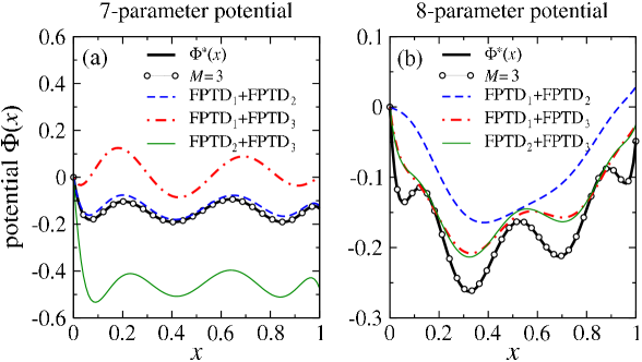
In figure 9 we successfully reconstruct 7-parameter and 8-parameter potential wells containing multiple minima using $g(s)=1$ and three ($M=3$) FPTDs. For both (a) the 7-parameter and (b) the 8-parameter potential, we see that any combination of two first passage time distribution data sets fails to accurately reproduce the original $\Phi^{*}(x)$. However, using the three defined data sets ($M=3$), we were able converge to the correct $\Phi^{*}(x)$ in fewer than 20 iterations. Importantly, we were able to quantitatively resolve the multiple minima. It should be noted, however, that with the current optimization algorithm we were only able to obtain about 2 significant digits of accuracy on the coefficients $a_{i}$ for these potentials.