Phenomenological analysis of D-brane Pati-Salam vacua

Abstract:

In the present work, we perform a phenomenological analysis of the effective low energy models with Pati-Salam (PS) gauge symmetry derived in the context of D-branes. The main issue in these models arises from the fact that the right-handed fermions and the PS-symmetry breaking Higgs field transform identically under the symmetry, causing unnatural matter-Higgs mixing effects. We argue that this problem can be solved in particular D-brane setups where these fields arise in different intersections. We further observe that whenever a large Higgs mass term is being generated in a particular class of mass spectra, a splitting mechanism –reminiscent of the doublet triplet splitting– may protect the neutral Higgs components from becoming heavy. We analyze the implications of each individual representation available in these models in order to specify the minimal spectrum required to build up a consistent model that reconciles the low energy data. A short discussion is devoted to the effects of stringy instanton corrections, particularly those generating missing Yukawa couplings and contributing to the fermion mass textures. We discuss the correlations of the intersecting D-brane spectra with those obtained from Gepner constructions and analyze the superpotential, the resulting mass textures and the low energy implications of some examples of the latter along the lines proposed above.

1 Introduction

Extended objects of the non-perturbative sector of string theory, the so-called D-branes [1, 2, 3], appears to be a promising framework for model building. Intersecting D-branes in particular, can provide chiral fermions and gauge symmetries, which contain the Standard Model spectrum and the $SU(3)\times SU(2)\times U(1)$ symmetry as a subgroup. The fermion and gauge fields are localized on the D-branes while gravity propagates in the bulk thus, D-brane models are natural candidates for phenomenological explorations. During the last years, particular supersymmetric or non-supersymmetric models have been proposed, based on various D-brane configurations, which exhibit a number of interesting properties.

Indeed, there are several remarkable features in these constructions that convincingly point towards a thorough investigation of promising D-brane derived models at low energy. An interesting property, for example, is that the multiplicity of the chiral sector and the strength of the Yukawa couplings are related to the geometry of the internal space. It has been also shown that instanton contributions play a vital rôle in the interpretation of the hierarchical mass spectrum. Furthermore, generically, the embedding of old successful Grand Unified Theories into D-brane configurations enhance the old GUT gauge symmetries by several $U(1)$ factors, while some of them remain at low energies as global symmetries. Interestingly, in certain occasions, there exist combinations of them, which can be identified with baryon or lepton conserving quantum numbers. At the String level, these abelian symmetries contain anomalies, which are canceled by a generalized Green-Schwarz mechanism. Usually, a linear combination of these $U(1)$’s remains anomaly free and plays a significant rôle in phenomenological investigations [4]-[11].

In this work, we discuss in some detail D-brane models based on the Pati-Salam (PS) symmetry [12]. The realization of this gauge model is assumed in the context of type IIA intersecting D6-brane models. However, the landscape of the string derived constructions is vast and it is not easy to select a viable vacuum. Thus, to ascertain the required characteristics and incorporate the low energy phenomenological constraints of the string derived construction, in the first part of this paper, we will start our analysis with a bottom up approach. This will help us to pin down the most promising models in Gepner constructions which will be discussed in the last sections.

As it is the case for all GUT models realized within the context of intersecting D-branes, the PS gauge group can also be accommodated within a larger gauge symmetry, namely

$$U(4)\times U(2)_{L}\times U(2)_{R}\cdot$$

Any gauge group factor $U(n)$ of the above symmetry contains a decoupled $U(1)$ component, and we can locally write $U(n)=SU(n)\times U(1)$. Therefore, one ends up with an extended PS symmetry accompanied by three $U(1)$ factors, which carry a strong impact on the superpotential of the effective low energy theory. Among other implications, they considerably restrict the trilinear terms available in the superpotential, while in particular cases, a certain combination of them is anomaly free and can be used to modify the hypercharge generator. In several cases, such a modification could occur without affecting the hypercharges of the Standard Model content while it might be used to provide integral charges to exotic states.

In what follows, we will present the emerging massless spectrum of the simpler D-brane configurations and determine the conditions under which realistic effective field theory models can be obtained. Next, as a testing ground of our general analysis, we will attempt to work out some semi-realistic examples derived from Gepner constructions where similar spectra arise.

In building up PS models from D-brane configurations, we are mainly faced with two problems. One arises from the fact that the right-handed fermions and the PS breaking Higgs $H,\bar{H}$ transform exactly in the same way under the non-abelian part of the gauge symmetry. Since Higgs representations usually appear in vector like pairs, we are led to unacceptable family and Higgs supermultiplets mixing. This mixing occurs via effective mass terms generated from the trilinear part of the superpotential, after some appropriate singlet fields develop non-zero vevs. A crucial observation in these models is that these representations can appear under two different $U(1)$ charges, depending on whether the relevant string-endpoint is attached to the $U(2)_{R}$ brane or its mirror. We will subsequently show that this fact can be used to discriminate between the Higgs and the right-handed fermions and avoid this way the Higgs-family mixing. The second difficulty is closely related to the first one. It is quite frequent that the representations accommodating the chiral matter are accompanied by anti-chiral fields, and only the net number ($\#$ of chiral minus $\#$ of anti-chiral) can be identified with the three generations required. Consequently, there is an excess of vector like pairs, which must become massive at a high ($\sim M_{GUT}$) scale and decouple from the low energy spectrum. Whatever mechanism is mobilized to make these pairs massive, it will also provide for a same order of magnitude mass term to the vector-like Higgs fields $H,\bar{H}$. We will discuss the available mechanisms which provide sufficiently large masses to the extraneous matter fields and, at the same time protect the Higgs field from receiving too large a mass. As an alternative scenario, we will propose a mechanism (reminiscent to the doublet-triplet splitting) which separates the charged particles from the neutral singlet, allowing the latter to develop a non-zero vev. This vev will prove useful to generate masses for the various states through tree-level and non-renormalizable Yukawa couplings.

The paper is organized as follows. In section 2, we briefly describe the basic set up of the $SU(4)\times SU(2)\times SU(2)$ (PS) gauge symmetry and discuss the minimal number of fields required to reproduce the low energy Standard Model (SM) spectrum. In section 3 we present the general features of the $U(4)\times U(2)\times U(2)$ D-brane analogue, paying particular attention to the new features and their implications. In particular, we consider the implications of the additional $U(1)$ symmetries in detail (as in comparison to the minimal PS gauge group) to the form of the superpotential couplings. We further discuss the implications of the extraneous representations which accompany the Standard Model spectrum. We present the possibilities of accommodating the SM spectrum in the D-brane intersections and exhibit the generic forms of the fermion mass textures for each case. We discuss the neutrino sector and give a short presentation of the possible stringy instanton generated masses whenever $U(1)$ symmetries or anomaly cancellation restrictions do not allow their explicit appearance in the perturbative superpotential. In section 4 we present the Higgs sector and discuss the possible patterns of symmetry breaking down to the Standard Model gauge symmetry. In section 5 we discuss the analogy between this generic D-brane spectra and comparable spectra derived from Gepner constructions, and apply the above analysis to specific examples. More details together with further examples of Gepner spectra are included in the appendices. Finally, in section 6 we present our conclusions.

2 A Minimal Model with PS Symmetry

In this section, we describe the minimal field theory version [13] of the model based on the Pati Salam (PS) gauge symmetry

$$SU(4)\times SU(2)_{L}\times SU(2)_{R}\cdot$$ (1)

This model has been extensively investigated in the context of the heterotic superstring and it was shown to possess several attractive features. Among them, we mention that this symmetry does not require the use of the adjoint or larger Higgs representations to be broken down to the SM, while the doublet-triplet splitting [14] is not an issue here, since the color triplets and the Higgs doublets are no longer members of the same multiplet. Furthermore, this model, in its minimal version, predicts unification of the third generation Yukawa couplings while the gauge couplings attain a common value at a scale as high as $M_{GUT}\sim 2\times 10^{16}$GeV.

The matter field content of the minimal model consists of the following representations. There are three chiral copies of $F_{L}$ and $\bar{F}_{R}$ multiplets transforming as the bifundamentals $(4,2,1)$ and $(\bar{4},1,2)$ respectively under the corresponding gauge symmetry factors in (1) which accommodate SM fields including the right-handed neutrino. Both multiplets are integrated in the $16$ of the $SO(10)$

$$16 \rightarrow (4,2,1)+(\bar{4},1,2)\cdot$$ (2)

Employing the hypercharge definition

$$Y=\frac{1}{2}\,Q_{B-L}+\frac{1}{2}\,Q_{3R}$$ (3)

where

$$Q_{3R}=\left(\begin{array}[]{cc}1&0\\ 0&-1\end{array}\right), Q_{B-L}=\left(\begin{array}[]{cccc}\frac{1}{3}&0&0&0\\ 0&\frac{1}{3}&0&0\\ 0&0&\frac{1}{3}&0\\ 0&0&0&-1\end{array}\right)$$ (10)

the Standard particle assignment is

$$F_{L} = ({4},{2},{1})=Q({3},{2},\frac{1}{6})+\ell{({1},{2},-\frac{1}{2})}$$ (11)

$$\bar{F}_{R} = (\bar{{4}},{1},{2})=u^{c}({\bar{3}},{1},-\frac{2}{3})+d^{c}({\bar{3}},{1},\frac{1}{3})+\nu^{c}({1},{1},0)+e^{c}({1},{1},1)\cdot$$ (12)

The $SU(4)\times SU(2)_{R}\rightarrow SU(3)_{C}\times U(1)_{Y}$ breaking can be realized with two Higgs fields $\bar{H}=(\bar{4},1,2)$ and $H=(4,1,2)$

$$\bar{H}=(\bar{4},1,2) = (u^{c}_{H},\,d^{c}_{h},\,e^{c}_{H},\,\nu^{c}_{H})$$ (13)

$$H=(4,1,2) = (\bar{u}^{c}_{H},\,\bar{d}^{c}_{h},\,\bar{e}^{c}_{H},\,\bar{\nu}^{c}_{H})$$ (14)

which descend from the $16$ and $\overline{16}$ of $SO(10)$ respectively

$$16_{\bar{H}} \rightarrow (4,2,1)+({\bar{4},1,2})$$ (15)

$$\overline{16}_{H} \rightarrow (\bar{4},2,1)+({4,1,2})\cdot$$ (16)

The particle assignment of $\bar{H}$ shares the same quantum numbers with $\bar{F}_{R}$, whilst that of $H$ shares the conjugate. Both acquire vevs along their sneutrino like components at a high scale

$$\langle H\rangle\,=\langle\bar{\nu}^{c}_{H}\rangle\,=\,M_{GUT}, \langle\bar{H}\rangle\,=\langle\nu^{c}_{H}\rangle\,=\,M_{GUT}\cdot$$ (17)

The SM symmetry breaking is realized by means of a bidoublet field $h=(1,2,2)$. This bidoublet constitutes part of the $10$ of $SO(10)$ which, under the PS-chain breaking gives $10\rightarrow D_{6}(6,1,1)+h(1,2,2)$. After the spontaneous breaking of the PS symmetry down to the SM, the sextets decompose to the usual triplet pair $D_{6}\rightarrow D_{3}+\bar{D}_{3}$, and the bidoublet to the two MSSM Higgs multiplets $h\rightarrow h_{u}+h_{d}$ which subsequently realize the SM breaking and provide masses to the fermions.

At the tree-level, all fermion species receive Dirac mass from a common Yukawa term $\bar{F}_{R}F_{L}h$. In the presence of a $U(1)$ family-like symmetry [15] (as is the case of heterotic string models for example), only the third generation receives tree-level masses, and, at the GUT scale, Yukawa unification is predicted

$$\lambda_{t}(M_{GUT})=\lambda_{b}(M_{GUT})=\lambda_{\tau}(M_{GUT})=\lambda_{\nu}(M_{GUT})\cdot$$ (18)

Furthermore, the PS symmetry implies the following mass relations at $M_{GUT}$

$$m_{t}(M_{GUT}) = m_{\nu}(M_{GUT})$$ (19)

$$m_{b}(M_{GUT}) = m_{\tau}(M_{GUT})$$ (20)

up to small threshold corrections. Smaller Yukawa contributions to the fermion masses arise from non renormalizable terms involving the Higgs fields $H,\bar{H}$ and, eventually, a neutral singlet vev $\phi$ charged under the $U(1)$ family symmetry. Majorana masses which realize the see-saw mechanism may arise from fourth order NR-operators and -depending on the particular $U(1)$ charge assignment- possible subleading terms of the form [15]

$$M_{\nu^{c}} \propto \frac{\bar{F}_{Ri}\bar{F}_{Rj}HH}{M_{GUT}},\;\frac{\bar{F}_{Ri}\bar{F}_{Rj}HH\phi}{M_{GUT}},\;\;\cdots$$ (21)

In the presence of sextet fields $D_{6}$, the trilinear superpotential terms $HHD_{6}+\bar{H}\bar{H}D_{6}$ provide the triplets $d_{H}^{c},\bar{d}_{H}^{c}$ (uneaten by the Higgs mechanism) with GUT-scale masses, by pairing them up with the triplets of $D_{6}$, $M_{GUT}d_{H}^{c}D_{3}$ and $M_{GUT}\bar{d}_{H}^{c}\bar{D}_{3}$ as follows:

$$HHD_{6}+\bar{H}\bar{H}D_{6}\rightarrow M_{GUT}d_{H}^{c}D_{3}+M_{GUT}\bar{d}_{H}^{c}\bar{D}_{3}\cdot$$ (22)

Having exhibited the salient features of the PS model, we now turn on to the D-brane version, which in its minimal form is obtained from a three-stack D-brane configuration leading to the enlarged $U(4)\times U(2)\times U(2)$ gauge group.

3 The D-brane Pati-Salam analogue

The D-brane realization of the PS symmetry requires a minimum of three stacks of branes [16]-[21]. Gauge fields are described by open strings with both endpoints attached on the same stack, and, they generically give rise to Unitary groups. The rest of the SM particles corresponds to open strings attached on different (or the same) stack providing bi-fundamental (as well as symmetric or antisymmetric) representations. The hypercharge is a linear combination of the abelian factors of each stack. In general, the other linear combinations of the abelian factors are anomalous. These anomalies are canceled by the Green-Schwarz mechanism and by generalized Chern-Simons terms [22]. The anomalous U(1) gauge bosons are massive and their masses can vary between the string scale and a much lower scale depending on the appropriate volume factors [23]. The $F_{L},~{}F_{R},~{}F_{L}^{\prime},~{}F_{R}^{\prime},~{}H,~{}H^{\prime}$ and their conjugates are described by strings with one end on the a-stack (the 4 branes stack), and the other on the b- or c-stacks (the 2 branes stacks). The $h,~{}h^{\prime}$ and their conjugates correspond to strings stretched between the b- and c-stack. Strings with one end on one stack and the other on the image stack, transform under symmetric or antisymmetric representations.

Table 1 shows all the possible representations that can be generated by strings stretched between the three brane-stacks and their corresponding mirrors. The appearance of any of these states in the model spectrum depends upon the particular choice of the intersections number which has to respect certain consistency conditions. In the intersecting D-brane scenario, for example, one has to ensure appropriate numbers of intersections, which lead to three chiral families and the disappearance of exotic matter. At the same time, the solutions should respect the constraints ensuring anomalies and tadpole cancelation [1, 2, 24].

Although several D-brane variants have so far appeared in the literature [25]-[30], a lot still remains to be done concerning a systematic investigation of the resulting effective low energy theory and its predictions. Up until now considerable work has been devoted to explore the implications of the heterotic analogue. However, the issue of the D-brane construction carries a separate interest of its own. The reason is that in comparison to the heterotic constructions, D-brane models contain new ingredients. These ingredients predict new states not previously available, that include the adjoints and various symmetric representations under the three gauge group factors of the PS symmetry. On the other hand, global $U(1)$ symmetries impose rather important restrictions on the superpotential couplings at low energies, remnants from the additional gauged abelian factors discussed earlier. Thus, given the aforementioned differences with other (heterotic string and orbifold) embeddings of the PS symmetry, the hope is that in working out a realistic brane model, the exotic matter would give a clear signal that could discriminate it from other string constructions. This way, we will consider a PS model carrying the general characteristics of these D-brane variants and discuss the implications, the viability and the prospects. In particular, we will attempt to specify the minimal spectrum and the properties required for obtaining a viable low energy effective field theory. In the next sections, we will also discuss the matching of the intersecting D-brane spectrum with spectra arising in certain Gepner constructions and analyze a number of semi-realistic examples [30].

Inters.	$SU(4)\times SU(2)_{L}\times SU(2)_{R}$	$Q_{4}$	$Q_{2L}$	$Q_{2R}$
$ab$	$(n+k)\times F_{L}\,(4,\bar{2},1)$	$1$	$-1$	$0$
	$n\times F_{L}\,(\bar{4},2,1)$	$-1$	$1$	$0$
$ab^{*}$	$(m+k^{\prime})\times F^{\prime}_{L}\,(4,2,1)$	$1$	$1$	$0$
	$m\times\bar{F}^{\prime}_{L}\,(\bar{4},\bar{2},1)$	$-1$	$-1$	$0$
$ac$	$\ell\times\bar{F}_{R}\,(\bar{4},1,2)$	$-1$	$0$	$1$
	$\bar{n}\times\bar{H}\,(\bar{4},1,2)$	$-1$	$0$	$1$
	$\bar{n}\times H\,(4,1,\bar{2})$	$1$	$0$	$-1$
$ac^{*}$	$\ell^{\prime}\times\bar{F}^{\prime}_{R}\,(\bar{4},1,\bar{2})$	$-1$	$0$	$-1$
	$\bar{m}\times\bar{H}^{\prime}\,(\bar{4},1,\bar{2})$	$-1$	$0$	$-1$
	$\bar{m}\times H^{\prime}\,(4,1,2)$	$1$	$0$	$1$
$aa^{*}$	$D_{6}\,(6,1,1)$	$\pm 2$	$0$	$0$
	$(S_{10},\bar{S}_{10})$	$\pm 2$	0	0
$cc^{*}$	$\Delta_{R}\,(1,1,3)$	$0$	$0$	$\pm 2$
	$(\phi,\bar{\phi})$	0	0	$\pm 2$
$bb^{*}$	$\Delta_{L}\,(1,3,1)$	$0$	$\pm 2$	$0$
	$(\nu_{s},\bar{\nu}_{s})$	$0$	$\pm 2$	$0$
$bc^{*}$	$\left.\begin{array}[]{c}h(1,2,2)\\ \bar{h}(1,\bar{2},\bar{2})\end{array}\right.$	$\left.\begin{array}[]{c}0\\ 0\end{array}\right.$	$\left.\begin{array}[]{c}1\\ -1\end{array}\right.$	$\left.\begin{array}[]{c}1\\ -1\end{array}\right.$
$bc$	$\left.\begin{array}[]{c}h^{\prime}(1,2,\bar{2})\\ \bar{h}^{\prime}(1,\bar{2},2)\end{array}\right.$	$\left.\begin{array}[]{c}0\\ 0\end{array}\right.$	$\left.\begin{array}[]{c}1\\ -1\end{array}\right.$	$\left.\begin{array}[]{c}-1\\ 1\end{array}\right.$

Table 1: The Spectrum and the corresponding quantum numbers emerging in a D-brane configuration with $U(4)\times U(2)\times U(2)$ gauge symmetry. $\ell,\ell^{\prime},k,k^{\prime},m,\bar{m},n,\bar{n}$ represent multiplicities of the corresponding states. By $a,~{}b,~{}c$ we denote the stacks of 4-, 2_L- and 2_R-stack of branes respectively and “*” denotes the mirror branes under the orientifold planes. Multiple numbers of fields may also arise in the remaining intersections $aa^{*}$, $bb^{*}$, $cc^{*}$, $bc$, $bc^{*}$.

3.1 The Superpotential

We start our discussion with the superpotential of the effective theory which at the perturbative level may receive tree-level contributions and higher order corrections. It is to be noted that in these constructions several tree-level superpotential terms of crucial importance are absent because of the surplus $U(1)$ symmetries. In addition, in several cases non-renormalization theorems can also prevent the appearance of non-renormalizable terms. In this case, stringy instanton effects [31]-[46] could compensate for the absence of the missing terms. This situation occurs usually in solutions with minimal spectra. In what follows, we make a detailed investigation of the perturbative and non-perturbative superpotential terms in order to pin down the minimal number of fields of Table 1 required to build a consistent model.

3.1.1 Perturbative superpotential

We first observe that in the PS model fermions belong to bifundamentals created by strings whose endpoints are attached on the branes with $U(4)$ and $U(2)_{L/R}$ factors. Left-handed fermions transform as $4\in SU(4)$ and are represented by strings attached on the $U(4)$ brane with $+1$ charge under the corresponding $U(1)$. Right-handed fermions transform as $\bar{4}\in SU(4)$ and carry $-1$ charge under the same abelian factor. We have more options for the other endpoint of the string. Since in $SU(2)$ doublets and antidoublets are indistinguishable, we may choose to attach the other endpoint of these strings either on the $U(2)$ branes or on their mirrors. Families attached to the $U(2)$ branes however, will differ from those attached to the mirrors with respect to the corresponding $U(1)_{L/R}$ factors. We may take advantage of this fact and make a suitable arrangement of the families to obtain the desired fermion mass hierarchy and meet all the related requirements of low-energy physics. We assume three families of left $F^{\prime}_{L},F_{L}$ and right $\bar{F}^{\prime}_{R},\bar{F}_{R}$ fields, thus, the multiplicities shown in Table must fulfill

$$k+k^{\prime}=\ell+\ell^{\prime}=3.$$ (23)

We also assume Higgs bidoublets $h,\bar{h}$ originating from the $bc^{*}$ intersection, corresponding to the two possible orientations of the string . Additional Higgs bidoublets (designated by $h^{\prime},\bar{h}^{\prime}$) may also arise from the $bc$ intersection.

The fermions of the three Standard Model families obtain their masses from gauge invariant couplings of the form $\bar{F}_{R}^{i}\,F_{L}^{j}\,h$. However, due to the $U(1)$ symmetries, some of these terms might not be allowed. Introducing indices for the representations with identical transformation properties, while assuming that the Higgs fields arise only in $bc^{*}$ intersection, (i.e., if only $h,\bar{h}$ exist), the available tree-level couplings are

$${\cal W} = \lambda_{im}\,\bar{F}^{\prime}_{R_{i}}F_{L_{m}}\langle h\rangle+\lambda^{\prime}_{nj}\bar{F}_{R_{n}}F^{\prime}_{L_{j}}\langle\bar{h}\rangle\cdot$$ (24)

If the $h^{\prime},\bar{h}^{\prime}$ bidoublet Higgses are also present, we may have the supplementary terms

$${\cal W}^{\prime} = y_{nm}\bar{F}_{R_{n}}F_{L_{m}}\langle\bar{h}^{\prime}\rangle+y^{\prime}_{ij}\,\bar{F}^{\prime}_{R_{i}}F^{\prime}_{L_{j}}\langle h^{\prime}\rangle\cdot$$ (25)

In the minimal case where we have no-extra vector like pairs $F_{L}\bar{F}_{L}$ and $\bar{F}_{R}F_{R}$, the various fermion masses are obtained by the usual $3\times 3$ matrices whose formal structure looks like

$$m_{u,d,\ell,\nu} \sim \left(\begin{array}[]{ll}y_{nm}\langle\bar{h}^{\prime}\rangle&\lambda_{nj}^{\prime}\langle\bar{h}\rangle\\ \lambda_{im}\langle h\rangle&y_{ij}^{\prime}\langle h^{\prime}\rangle\end{array}\right)$$ (28)

where the various indices $i,j,m,n$ take the appropriate values.

As we will soon see, the presence of both kinds of bidoublet Higgs fields ($ac$ and $ac^{*}$) generates a number of undesired Yukawa couplings. Therefore, in a rather realistic construction, we should be able to accommodate only one kind of Higgs, (say $h$ and/or $\bar{h}$). In this case, we distinguish between the following distinct non-trivial classes of mass matrices.

• If all the left handed representations arise from the $ab$ sector and the right-handed ones from the $ac^{*}$ intersection, the only surviving term is $\lambda_{im}\,\bar{F}^{\prime}_{R_{i}}F_{L_{m}}\langle h\rangle$ and the mass matrices take the form

  $$m_{u,d,\ell,\nu} \sim \left(\begin{array}[]{lll}\lambda_{11}&\lambda_{12}&\lambda_{13}\\ \lambda_{21}&\lambda_{22}&\lambda_{23}\\ \lambda_{31}&\lambda_{32}&\lambda_{33}\end{array}\right)\langle h\rangle\cdot$$ (32)

• As a second possibility we consider the case where the left-handed fields arise from both the $ab$ and $ab^{*}$ sectors, $F_{1L}^{\prime},F_{2L},F_{3L}$, with all the right-handed ones descending from the $ac^{*}$ intersection. Now, we get

  $$m_{u,d,\ell,\nu} \sim \left(\begin{array}[]{lll}0&0&0\\ \lambda_{21}&\lambda_{22}&\lambda_{23}\\ \lambda_{31}&\lambda_{32}&\lambda_{33}\end{array}\right)\langle h\rangle\cdot$$ (36)

  In addition, two more cyclic permutations of the above matrix can be obtained by interchanging the generation indices. A comment is here in order. The PS gauge symmetry implies in all cases the same texture form for the up and down quarks. Higher order corrections are expected to discriminate between up and down quark mass matrices and create the desired Cabibbo-Kobayashi-Maskawa (CKM) mixing. We note that this is in contrast to some cases [51]-[55] which arise in the context of SM gauge symmetry where the up and down quark mass matrices have a ‘complementary’ texture-zero structure making it hard to reconcile the CKM mixing [58].

• As a final possibility, we consider the case of $F_{1L}^{\prime},F_{2L},F_{3L}$, and $F_{1R},F_{2R}^{\prime},F_{3R}^{\prime}$ combination which leads to the following texture

  $$m_{u,d,\ell,\nu} \sim \left(\begin{array}[]{lll}0&\lambda_{12}\langle h\rangle&\lambda_{13}\langle h\rangle\\ \lambda^{\prime}_{21}\langle\bar{h}\rangle&0&0\\ \lambda^{\prime}_{31}\langle\bar{h}\rangle&0&0\end{array}\right)\cdot$$ (40)

  In general, the above tree-level mass matrices contain several zeros which are expected to be filled by contributions coming from non-renormalizable terms or instantons.

The above textures deserve some discussion. In case A, we have seen that the specific choice of field accommodation has led to a mass texture where all the entries appear at the tree-level of the perturbative superpotential. In this case, it is expected that all Yukawa couplings $\lambda_{ij}$ are of the same order of magnitude. In such a texture, the hierarchical pattern will be rather difficult to explain in a natural way. Case B leads to a texture zero mass matrix with three zeros in the first row. Due to the PS symmetry, there is a unique gauge invariant Yukawa coupling to account for the fermion mass matrices, thus, we end up with the same texture for all kinds of fermions, namely up, down, charged leptons and Dirac neutrinos. Since non-perturbative contributions and/or NR-terms are expected to fill the gaps, and these contributions are naturally suppressed as compared to tree-level terms, this texture looks more realistic than the case A. Finally, the structure of case C is rather peculiar and probably less suitable for the charged fermion mass spectrum.

Let us now deal with the $SU(4)$ breaking Higgs fields. These may arise at the $ac$ and $ac^{*}$ intersections and are denoted by $H+\bar{H}$, and $H^{\prime}+\bar{H}^{\prime}$ respectively. Since $\bar{H},\bar{H}^{\prime}$ carry exactly the same quantum numbers as $\bar{F}_{R_{i}},\bar{F}^{\prime}_{R_{i}}$ correspondingly, we must also have the couplings

$${\cal W}^{\prime\prime} = \lambda_{ij}\,\bar{H}^{\prime}\,F_{L_{j}}\,h+\lambda^{\prime}_{ij}\bar{H}\,F^{\prime}_{L_{i}}\,\bar{h}\cdot$$ (41)

In order to break the $SU(4)\times SU(2)_{R}$ symmetry, we have to assign vevs either to $H+\bar{H}$, or to $H^{\prime}+\bar{H}^{\prime}$. Allowing the RH fields to descend from both $ac$ and $ac^{*}$ intersections, anyone of the $\bar{H},\bar{H}^{\prime}$ vevs will render at least one lepton and one Higgs doublet massive at an unacceptably large scale

$$\lambda_{ij}\,\langle\bar{H}^{\prime}\rangle\,F_{L_{j}}\,h \rightarrow M_{GUT}\ell_{j}h_{u}$$ (42)

$$\lambda_{ij}\,\langle\bar{H}\rangle\,F^{\prime}_{L_{j}}\,\bar{h} \rightarrow M_{GUT}\ell^{\prime}_{j}\bar{h}_{u}\cdot$$

This problem may be evaded by assuming that the $SU(4)$ breaking Higgs and the representation $\bar{F}_{R}$ accommodating the right-handed fields have distinct quantum numbers under $U(1)$ symmetries. This is possible under the following arrangement:

First, we will assume that all three representations $(4,2,1)$ accommodating the left handed fields arise in the $ab$ intersection, thus $k=3,k^{\prime}=0$. We will further demand that the right-handed fields are only at the $bc^{*}$ intersection thus $\ell=0,\ell^{\prime}=3$. Then, only the first tree-level coupling in (24) is present at ${\cal W}$:

$$\lambda_{ij}\,\bar{F}^{\prime}_{R_{i}}F_{L_{j}}\,h \rightarrow Q\,u^{c}\,\langle h_{u}\rangle+\ell\,\nu^{c}\,\langle h_{u}\rangle+Q\,d^{c}\,\langle h_{d}\rangle+\ell\,e^{c}\,\langle h_{d}\rangle\cdot$$ (43)

Next, in order to avoid undesired similar couplings, we will impose $\bar{m}=0$, and $\bar{n}\neq 0$ (preferably $\bar{n}=1$), so we have only $H+\bar{H}$ pairs, which carry different $U(1)$ charges from $\bar{F}^{\prime}_{R_{i}}$’s. This choice prevents the appearance of the unwanted couplings (42).

The $SU(4)$ breaking Higgs fields $H+\bar{H}$ involve $\bar{u}_{H}^{c},u_{H}^{c},\bar{e}_{H}^{c},e_{H}^{c}$ ‘eaten’ by the Higgs mechanism, and ‘uneaten’ down-quark type color triplets $\bar{d}_{H}^{c},d_{H}^{c}$ which must become massive at a high scale. In the presence of the sextet fields $D_{6}=D_{3}+D^{c}_{3}$ and $\bar{D}_{6}=\bar{D}_{3}+\bar{D}^{c}_{3}$, the simplest way to realize this is via couplings of the form $HH\bar{D}_{6},\bar{H}\bar{H}D_{6}$, which in the intersecting D-brane scenarios are not allowed by the $U(1)$ symmetries at the tree-level. Fortunately, there are alternative ways to obtain masses for the triplets in these constructions. These involve the inclusion of non-renormalizable terms in the presence of additional singlet fields, which develop appropriate vevs and/or, possible instanton effects.

We start with the first approach. We observe that the singlet fields $\phi,\bar{\phi}$ arising from the $cc^{*}$ sector and presented in Table 1, have the appropriate $U(1)$ charges to generate the fourth order terms

$$\frac{\phi}{M_{S}}\,HH\,\bar{D}_{6},\;\;\frac{\bar{\phi}}{M_{S}}\,\bar{H}\bar{H}D_{6}\cdot$$ (44)

Upon developing vevs $\langle\phi\rangle\sim\langle\bar{\phi}\rangle\sim M_{GUT}$, the singlet fields generate the missing mass terms for the triplets. We should point out however, that possible non-zero vevs for these singlets, would generate undesired effects as it is the case, for example, for the term $\bar{F}_{R}\,\phi\,H$. In such cases, we are forced to set $\langle\phi\rangle=0$ nevertheless we will see that it is possible to derive the mass terms (44) by instanton effects.

To determine the final form of the down-type colored triplet sector, one should also encounter the terms $\bar{H}\,\bar{F}^{\prime}_{R}\,D_{6}$ and $H\,F_{L}\,\bar{D}_{6}\,h$ which mix the down quarks in $\bar{F}^{\prime}_{R}$ with the triplet fields living in $D_{6},\,\bar{D}_{6}$, leading thus to an extended down quark mass matrix. Higher order non-renomalizable terms may also contribute to the generalized down quark mass matrix, which, under a judicious choice of the various field vevs for $\phi,H,\bar{H}$ can leave three light eigenstates to be identified with the ordinary down quarks.

Proceeding with the analysis, we recall that as opposed to the minimal field theory version presented previously, in D-brane constructions there exist additional states, which belong to the symmetric and/or antisymmetric representations of each non-abelian gauge group factor. These are designated by $S_{10},\bar{S}_{10}$ for the $SU(3)$ case and $\Delta_{L,R}$ for the $SU(2)_{L,R}$ respectively. The additional $SU(2)_{R}$ triplets have the particle assignment $\Delta_{R}(1,1,3)=(\delta^{+},\delta^{0},\delta^{-})$, or

$$\tau\cdot{\Delta}_{R} = \left(\begin{array}[]{cc}\frac{\delta^{0}}{\sqrt{2}}&\delta^{+}\\ \delta^{-}&-\frac{\delta^{0}}{\sqrt{2}}\end{array}\right)$$ (47)

and analogously for the $\Delta_{L}(1,3,1)$ ones. Also, the $S_{10}$ SM-decomposition involves

$$S_{10} \rightarrow S_{6}(6,-\frac{2}{3})+S_{3}(3,\frac{2}{3})+S_{1}(1,2)$$ (48)

where the triplet field $S_{3}$ carries the quantum numbers of the down quarks. We will see that in cases where more conventional representations (i.e., the neutral singlets and color sextet fields $D_{6}$) are absent from the massless spectrum, the fields (47) and (48) provide supplementary terms in the superpotential which can act as surrogates to make the color triplets in $H,\bar{H}$ Higgs fields massive, or even realize the see-saw mechanism.

Indeed, in models containing the representations $S_{10}$ and $\bar{S}_{10}$ we may also have the trilinear couplings

$$H\,H\,\bar{S}_{10}+\bar{H}\,\bar{H}\,S_{10} \rightarrow M_{GUT}\,(\bar{d}_{H}^{c}\,\bar{S}_{3}+d_{H}^{c}\,S_{3})\cdot$$ (49)

The fields $S_{10}$ and $\bar{S}_{10}$, under the Standard Model gauge group decomposition involve also other exotic representations, which should become massive at a high scale. This can be realized by a mass term $M_{10}S_{10}\bar{S}_{10}$ generated by a superpotential term where an effective scalar component $\phi_{0}$ acquires a non-zero vev at a scale $\langle\phi_{0}\rangle\sim M_{GUT}$. In this case, a term $M_{GUT}\bar{S}_{3}S_{3}$ is also implied which, in conjunction with the mass terms (49) form a triplet mass matrix with eigenmasses being naturally of the order $M_{GUT}$.

Finally, we also comment on the existence of an additional Higgs pair $h^{\prime}+\bar{h}^{\prime}$ in the intersection $bc$. Denoting $h^{\prime}=h_{u}^{\prime}+h_{d}^{\prime}$ and $F_{L}=Q+\ell$, we observe that the coupling

$$\bar{H}F_{L}h^{\prime} \rightarrow \langle\nu_{H}\rangle\,\ell\,h_{u}^{\prime}$$ (50)

couples the lepton doublet $\ell$ with $h_{u}^{\prime}$ through a mass of the order of GUT scale. We could be further elaborate on this case by constructing the full doublet mass matrix, taking into account possible non-renormalizable terms, and seek solutions with three light doublets in analogy to the down quark mass matrix discussed above. This line, however, would lead to a rather contrived model, thus, it is more natural to assume the simpler case with only one light bidoublet Higgs $h$ and/or $\bar{h}$.

3.1.2 Neutrino masses

In PS models right-handed neutrinos are incorporated into the same representation with the right-handed charged fermions. They receive Dirac masses through the same term (24) sharing the same Higgs doublet with the up-quarks. Therefore, the Dirac neutrino masses are of the same order of magnitude with the up quark masses and a see-saw mechanism is required in order to generate light Majorana mass eigenstates compatible with the present experimental bounds.

In the presence of the fields $\Delta_{R}$ and $\phi$, an extended see-saw mechanism can generate light Majorana masses through the following tree level terms

$$\lambda^{\prime}_{\nu^{c}}\bar{F}^{\prime}_{R_{i}}\Delta_{R}\,H+\lambda_{\nu^{c}}\bar{F}^{\prime}_{R}\,\phi\,H \to \langle\tilde{\bar{\nu}}_{H}^{c}\rangle\delta^{0}{\nu^{\prime}}^{c}+\langle\tilde{\bar{\nu}}_{H}^{c}\rangle\,\phi\,{\nu^{\prime}}^{c}$$ (51)

with $\delta^{0}\in\Delta_{R}$. Either one of these terms is sufficient to realize the see-saw mechanism. We also note that in the presence of $\bar{\phi}$ singlets, non-renormalizable mass terms contributing to the neutrino mass matrix are also possible

$$\frac{\bar{F}^{\prime}_{R}\bar{F}^{\prime}_{R}HH\bar{\phi}}{M_{GUT}} \sim M_{nr}{\nu^{\prime}}^{c}{\nu^{\prime}}^{c}\cdot$$ (52)

Suppressing generation indices, the complete tree-level neutrino mass matrix in the basis $\nu_{i},\nu_{i}^{c}$, and $\delta^{0}$ (and/or $\phi$) can be written as

$$M_{\nu} \sim \left(\begin{array}[]{lll}0&m_{u}&0\\ m_{u}&M_{nr}&M\\ 0&M&0\end{array}\right)\cdot$$ (56)

Thus, taking into account all the contributions to neutrinos and other neutral states, we end up with the extended see-saw type mass matrix (56) which leads to three light left-handed neutrino states, which can naturally lie in the sub-eV range as required by the present neutrino data.

3.1.3 Instanton induced masses

We have seen in the previous sections, that for certain cases of D-brane spectra, several Yukawa couplings of crucial importance are absent from the tree level superpotential. For example, in the absence of the $h^{\prime}+\bar{h}^{\prime}$ bidoublets we noticed that Yukawas implying $\bar{F}_{R}F_{L}$ and $\bar{F}_{R}^{\prime}F_{L}^{\prime}$ mixings are not possible. Similarly, the terms $HHD_{6}$ and $\bar{H}\bar{H}D_{6}$ are prevented by global $U(1)$ symmetries leaving the dangerous color triplets massless. Furthermore, in the absence of appropriate singlet scalar fields with non-vanishing vevs, non-renormalizable contributions are impossible.

It has been suggested [33, 35, 36] that for a matter fields operator $\prod_{j}\Phi_{a_{j}b_{j}}$ violating the $U(1)$ symmetry, it is possible that Euclidean D2 (${\cal E}2$ for short) instantons having the appropriate number of intersections with the $D6$-branes can induce non-perturbative superpotential terms of the form

$${\cal W}_{n.p.} \supset \prod_{j=1}^{J}\Phi_{a_{j}b_{j}}\,e^{-S_{\cal E}}\cdot$$ (57)

In other words, the perturbatively forbidden Yukawa coupling is now realized non perturbatively, since in the presence of appropriate instanton zero modes, the instanton action $S_{\cal E}$ can absorb the $U(1)_{a}$ charge excess of the field operator violating the $U(1)$ symmetry. Indeed, under the $U(1)_{a}$ symmetry the transformation property of the exponential instanton action is

$$\,e^{-S_{\cal E}} \rightarrow \,e^{-S_{\cal E}}\,e^{\imath\,{\cal Q}_{a}({\cal E}2)\Lambda_{a}}$$ (58)

where ${\cal Q}_{a}({\cal E}2)$ represents the amount of the $U(1)_{a}$-charge violation by the ${\cal E}2$ instanton. If $\pi_{a},\pi_{a^{*}}$ are the homological three-cycles of the $D6_{a}$ brane-stack and its mirror respectively, then this is given by

$${\cal Q}_{a}({\cal E}2) = -{\cal N}_{a}\,\pi_{\cal E}\circ(\pi_{a}-\pi_{a^{*}})\equiv-{\cal N}_{a}\,(I_{{\cal E}a}-I_{{\cal E}{a^{*}}})$$ (59)

where the $I_{{\cal E}a}$ and $I_{{\cal E}{a^{*}}}$ stand for the relevant intersection numbers. For rigid $O(1)$ instantons, wrapping a rigid orientifold-invariant cycle in the internal space, due to the ${\cal E}2-a$ and ${\cal E}2-a^{*}$ identification the charge (59) simplifies to

$${\cal Q}_{a}({\cal E}2) = -{\cal N}_{a}\,\pi_{\cal E}\circ\pi_{a}\equiv-{\cal N}_{a}\,I_{{\cal E}a}$$ (60)

Thus, allowing for an appropriate number of wrappings, the above can exactly match the $U(1)_{a}$ charge excess of the filed operator $\prod_{j}\Phi_{a_{j}b_{j}}$ and the total coupling (58) is $U(1)_{a}$-invariant.

   

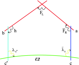
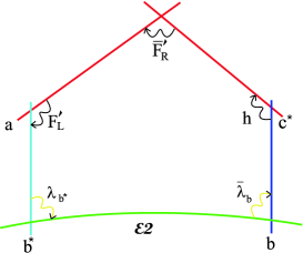
Figure 1: Stringy instanton generated Yukawa coupling $F_{R}F_{L}h,\,F_{R}^{\prime}\,F^{\prime}_{L}\,h$.

Returning to our specific model discussed here, we can, for example, observe that when $h^{\prime},\bar{h}^{\prime}$ bidoublets related to the intersection $bc$, are not found in the massless spectrum, the couplings (25) are not available. It is then possible that the zero entries in the fermion mass matrices discussed in the previous section, are filled by the instanton contributions (see fig 1)

$${\cal W}_{n.p.} = \lambda_{1}^{np}\,F_{R}F_{L}h+\lambda_{2}^{np}\,F_{R}^{\prime}\,F^{\prime}_{L}\,h\cdot$$ (61)

The induced coupling (57) involves an exponential suppression by the classical instanton action ${\cal W}_{n.p.}\propto\exp\{-\frac{8\pi^{2}{\rm Vol}_{\cal E}}{g_{a}^{2}{\rm Vol}_{D6_{a}}}\}$. This way, the couplings $\lambda_{1,2}^{np}$ are suppressed by exponential factors involving the classical instanton action, and are expected to be much smaller than the perturbative ones.

$$\lambda_{i}^{n.p.} \sim {\cal O}\left(e^{-S_{\cal E}}\lambda_{i}\right)\cdot$$ (62)

Note that other instantons can generate additional contributions to the same fermion zero entries, inducing factorizable Yukawa couplings instead of (61). This latter type of couplings appears also for the sextets fields. In particular, the zero mode wrapping conditions $I_{{\cal E}a}=1$ and $I_{{\cal E}b}=-1$ allow for the coupling $HHD_{6}$. Similar instanton effects with the appropriate winding numbers may generate couplings of the form $\bar{H}\bar{H}D_{6}$. We should remark however, that when both terms are present, potentially dangerous dimension five proton decay operators are generated as it was also observed in [43, 52, 54]. A crucial rôle is then played by the the scale at which the triplets $D_{3},\bar{D}_{3}\subset D_{6}$ become massive.

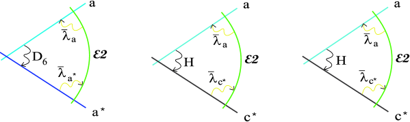
Figure 2: Stringy instanton generated Yukawa coupling $HHD_{6}$ giving mass to the color triplets.

4 The Higgs Sector and the right-handed “Doublet-Triplet” splitting

We have already pointed out that a rather general phenomenon in these constructions is the appearance of extra matter fields beyond those contained in the Standard Model. Our interest in the present section will focus on the extraneous matter related to the Higgs problem mentioned in the introduction. This particular extra matter comes in vector like pairs. Such a case was already encountered in the previous section, namely the $SU(3)$ non-trivial states $S_{10}+\bar{S}_{10}$. The most common case consists of the representations accommodating the same chiral fields themselves. Indeed, as it is generally shown in the Table, one might have $n+3$ chiral states in $F_{L}$ and $n$ states in $\bar{F}_{L}$, thus the net number of chiral supermultiplets is three; however, there are $n\neq 0$ copies of vector-like representations $F_{L}+\bar{F}_{L}$ since it is rather difficult in practice to derive a D-brane spectrum with $n=0$. The same is also true for the right handed partners $F_{R},\bar{F}_{R}$ which in addition to the three chirals $\bar{F}_{R}$ may also have an excess of several $\bar{F}_{R}+F_{R}$ copies. In a viable effective field theory model, all these states should decouple at a high scale. A natural mechanism to deal with this situation is to allow a non-zero vev to a singlet field that couples to these states $\langle\phi_{0}\rangle(\bar{F}_{L}F_{L}+\bar{F}_{R}F_{R}+\dots)$, $\langle\phi_{0}\rangle\sim M_{GUT}$, in order to avoid large threshold effects in the renormalization group (RG) running of precisely measured quantities at $M_{W}$ (i.e., $\sin^{2}\theta_{w},a_{em},a_{s}$ etc). In this case, it is unavoidable that a mass term $M_{GUT}H\bar{H}$ is generated, implying that the $H,\bar{H}$ fields decouple from the spectrum and cannot develop vevs along their neutral components. Another complication related to the same Higgs fields emerges from the fact that $\bar{H}$ and $\bar{F}_{R}$ transform identically under the PS symmetry, sharing thus the same Yukawa couplings and leading to the unacceptable matter-Higgs mixing already discussed in the previous sections. In what follows, we will suggest a solution to avoid these problems.

We start with the second issue. Taking the previous analysis at face value, we infer that in order to avoid undesired mixings, the RH fields $\bar{F}_{R}$ should not share the same Yukawa couplings with the Higgs $\bar{H}$. Since both of them transform equivalently under the non-abelian part of the gauge symmetry, they can only differ with respect to the $U(1)_{R}$ gauge factor. Thus, we may choose all RH-fermions from the $ac^{*}$ sector and pick up the $SU(4)$ breaking Higgs pair from the $ac$ intersection. This arrangement solves the problem of large unacceptable $H\bar{F}_{R}$ mixing. However, both $H,\bar{H}$ Higgs come from the same intersection with opposite $U(1)$ charges as indicated in the Table. If no extra matter in vector-like form is present in the spectrum of the theory, then there is no need for developing non-zero singlet vevs which could couple to the Higgs pair $\bar{H}H$. Consequently, the Higgs fields remain in the massless spectrum of the theory and their rôle as discussed in the previous sections remains intact.

We have argued that quite often vector-like fields are unavoidable, while consistency with low energy data requires that these should decouple from the light spectrum at a high scale. The most natural candidate mass terms for the extra pairs may arise at fourth order and can be of the form

$$\frac{\langle\bar{H}H\rangle}{M_{S}}\left(\bar{F}_{L}F_{L}+\bar{F}_{R}F_{R}+\bar{S}_{10}S_{10}+\bar{H}H+\bar{h}h+\cdots\right)\cdot$$ (63)

Assuming vevs of the Higgs fields along the D-flat direction, we naturally expect them to be of the order $\langle H\rangle\sim\langle\bar{H}\rangle\sim 10^{-1}M_{S}$ leading to an adequately large mass $M\sim 10^{-1}M_{GUT}$ for all extra matter. Unfortunately, a large number of such fields would generate sizable threshold effects in the renormalization group running of the gauge couplings, spoiling this way the unification prediction.

As an alternative to the NR-contributions we can let a singlet develop a non-zero vev $\langle\phi_{0}\rangle\sim M_{GUT}$ but as already discussed above, this would lead into the problem of a similar Higgs mass term. Below, we present a mechanism that could resolve this problem. In this case, whenever a mass term for $\bar{F}_{L}F_{L}$, $\bar{F}_{R}F_{R}$ is generated, the $U(1)$ symmetries cannot prevent the appearance of the analogous mass term for the Higgs pair $M_{H}\,H\bar{H}$, where $M_{H}$ is naturally of the order of the Unification scale $M_{GUT}$. Note that in the presence of an $SU(4)$ adjoint Higgs field $\Phi_{4}$, the following terms are allowed;

$${\cal W}_{H}\supset\bar{H}\,\Phi_{4}\,H+M_{H}\,\bar{H}\,H\cdot$$ (64)

We may now solve the problem by allowing the $SU(4)$-adjoint scalar $\Phi_{4}$ to obtain a vacuum expectation value which cancels the $M_{H}$ term. The $SU(4)$ adjoint is

$$(15,1,1) = \left(\begin{array}[]{cc}A_{8}-\frac{A_{0}}{2\sqrt{3}}\times{\bf 1}_{3}&B\\ \bar{B}&\frac{\sqrt{3}}{2}A_{0}\end{array}\right)\cdot$$ (67)

On the left-hand side of the above we explicitly indicate the transformation of the adjoint representation under the $SU(4)\times SU(2)_{L}\times SU(2)_{R}$ gauge symmetry. Take $v=-\langle\frac{\sqrt{3}A_{0}}{2}\rangle$, so that

$$\langle\Phi_{4}\rangle = \left(\begin{array}[]{cccc}\frac{v}{3}&0&0&0\\ 0&\frac{v}{3}&0&0\\ 0&0&\frac{v}{3}&0\\ 0&0&0&-v\end{array}\right)\cdot$$ (72)

The resulting mass terms from (64) are written as

$${\cal W}_{H}\supset\left(M_{H}-{v}\right)\,{\bar{L}}_{H}^{c}\,L_{H}^{c}+\left(\frac{v}{3}+M_{H}\right)\bar{Q}^{c}_{H}\,Q^{c}_{H}$$ (73)

where $Q^{c}_{H}=(u_{H}^{c},d^{c}_{H})^{T}$, $L^{c}_{H}=(e_{H}^{c},\nu^{c}_{H})^{T}$ are $SU(2)_{R}$ doublets. Clearly, because of the trivial transformation properties of the $SU(4)$ adjoint under the $SU(2)_{L/R}$ gauge groups (see (67), left-hand side), the corresponding gauge group factors are preserved. The choice $v\sim M_{H}$ would leave the right-handed doublets ${\bar{L}}^{c}_{H},\,L_{H}^{c}$ of $H,\bar{H}$ massless, while at the same time would supply all additional color particles with heavy masses $M\sim\frac{4}{3}M_{H}$ and break the original symmetry down to a left-right symmetric model

$$SU(3)\times SU(2)_{L}\times SU(2)_{R}\times U(1)_{B-L}\cdot$$

Thus, in this scenario, the PS symmetry breaking can occur in two steps. The vev $\langle\Phi_{4}\rangle$ realizes the $SU(4)$ symmetry breaking while, the vevs of the RH doublets ${\bar{L}}_{H}^{c},\,L_{H}^{c}$ along their neutral directions can break the $SU(2)_{R}$ symmetry. Although, in principle, these two breaking scales could differ substantially, purely phenomenological requirements demand that the $SU(2)_{R}$ breaking scale should not be much lower than the $SU(4)$ scale. Indeed, this arrangement permits several tree-level and NR-terms to generate useful mass contributions for the various SM fields, when $H,\bar{H}$ fields are allowed to acquire vevs along the neutral directions. If the $SU(2)_{R}$ breaking scale is substantially smaller than $M_{GUT}$, these contributions would be suppressed and therefore, become irrelevant. Since the natural expansion parameter in NR contributions is $\epsilon\sim\frac{\langle\bar{H}H\rangle}{M_{S}}$, we may assume that $\langle H\rangle\sim\langle\bar{H}\rangle\sim v\sim M_{GUT}$, thus $\epsilon$ takes natural values $\epsilon\sim{\cal O}(10^{-1})$. This estimate is quite reasonable and is not in conflict with the Renormalization Group analysis of the field theory model. Indeed, for mass spectra not deviating considerably from the minimal one, renormalization group analysis shows [57] that the magnitude of these $SU(4)$-breaking vevs cannot differ substantially from the standard SUSY GUT scale $M_{GUT}\sim(2-3)\times 10^{16}$ GeV. Taking into account that $M_{String}\approx 2\times 10^{17}$ GeV, we conclude that $M_{U}/M_{S}\sim 10^{-1}$. On the other hand, the various $M_{GUT}$ vevs including those of the $SU(4)$ breaking Higgs fieds $\langle\bar{H},H\rangle$ are related to the FI terms and their values depend on the various moduli. The solutions for particular Gepner models to be discussed later on show consistency with the above estimates.

From the last term in (63) we observe that in general there exist analogous effective mass terms for the light Higgs bidoublet fields as well. These couplings remove pairs $h_{i},\bar{h}_{i}$ of left-handed doublets from the light spectrum. To implement the $SU(2)_{L}$ symmetry breaking and provide fermions with masses, we need at least the content of one bidoublet Higgs $h\rightarrow h_{u}+h_{d}$ in the massless spectrum. Since bidoublet fields include both electroweak Higgs doublets, they are not necessarily required to appear in pairs $h,\bar{h}$. So, by arranging that the number $n_{h}$ of $h$’s does not coincide with the number $n_{\bar{h}}$, of $\bar{h}$ fields, a number of $|n_{h}-n_{\bar{h}}|$ bidoublets could, in principle, remain massless. As it will become evident in the next sections, this is exactly the case for the several examples obtained in the Gepner constructions. Also, in the case of $n_{h}=n_{\bar{h}}$ a splitting mechanism analogous to the $SU(4)$ case described above could be activated for the bidoublets where now the rôle of $\Phi_{4}$ is played by the vev of an $SU(2)_{R}$ triplet $\Delta_{R}$ or the adjoint $\Phi_{2R}$ . Implementing this mechanism, while assuming $\langle\Phi_{2R}\rangle={\rm diag}(v_{R},-v_{R})$, we obtain

$${\cal W}_{h} \supset \left(\frac{\langle H\bar{H}\rangle}{M_{S}}-v_{R}\right)h_{u}\bar{h}_{d}+\left(\frac{\langle H\bar{H}\rangle}{M_{S}}+v_{R}\right)\bar{h}_{u}h_{d}$$ (74)

with $\langle H\bar{H}\rangle\sim M_{GUT}^{2}$ as above. Hence, to ensure a massless electroweak pair $h_{u},\bar{h}_{d}$, we must impose the geometric mean relation $M_{GUT}\sim\sqrt{M_{S}\,|v_{R}|}$.

In the more general situation where there are several Higgses (as is often the case in realistic constructions), (64) generalizes to

$${\cal W}_{H} \supset \sum_{i,j}\bar{H}_{j}\,\Phi_{4}\,H_{i}+M_{H_{ij}}\,\bar{H}_{i}\,H_{j}$$ (75)

$$+ \sum_{i,j}\bar{H}_{i}^{\prime}\,\Phi_{4}\,H_{j}^{\prime}+M_{H_{ij}^{\prime}}\,\bar{H}_{i}^{\prime}\,H_{j}^{\prime}\cdot$$

Now, the mass terms in (73) become mass matrices and one has to seek conditions for the existence of zero eigenvalues in the ${\bar{L}}^{c}_{H_{i}},\,L_{H_{i}}^{c}$ mass matrix.

5 Pati Salam models at Gepner points

In the context of orientifolds constructed from Gepner models there has been an extensive search for all possible embeddings of the SM gauge theory in D-brane configurations [30, 52]. Among them, there are several cases where the SM is consistently embedded in a unified gauge group. The predicted spectrum in these models includes all SM matter representations, and the gauge couplings naturally unify at scales $M_{GUT}\sim 10^{16}$GeV. Successful candidate groups include $SU(5)$, flipped $SU(5)$, Pati-Salam gauge symmetry and trinification models. Studies to identify semi-realistic unified models based in $SU(5)$ symmetry had appeared as well  [52]. In what follows, we elaborate on two characteristic examples with the PS gauge group chosen from the pool of models derived in [30, 52] which have been found in the context of Gepner constructions. Guided by our previous phenomenological analysis, we pick up characteristic cases with massless spectra fulfilling most of the aforementioned requirements. First, we will deal with a model possessing extra states. This does not necessarily mean that the model is ruled out, however a number of refinements are necessary in order to overcome some of the problems discussed previously. As a second example, we choose a model with a minimal spectrum which inherits several of the nice features discussed above.

For both models we will present a phenomenological analysis of the superpotential, the fermion mass spectrum as well as related phenomenological issues. Doing so, we will need to make several mild assumptions about the parameter space. We should not forget however, the rather subtle issue of moduli stabilization , that might affect the freedom of choice for parameters used in this analysis. We will tacitly assume that a stabilization mechanism does exist, so we will mainly concentrate on the general forms and values for parameters in order to get semi-realistic realizations. We further note that there exists no explicit computation of Yukawas for orientifold models at Gepner points. This way, our superpotential is constrained by gauge invariance only, without taking into account conformal invariance restrictions that might shorten its length. This is not necessarily a shortcoming since several problematic gauge invariant couplings would probably be eliminated.

5.1 First Example

Here, we present a vacuum with a Pati-Salam-like massless spectrum that consists of the minimal configuration of three brane-stacks. In this model, the internal sector consists of a tensor product of five copies of ${\cal N}=2$ superconformal minimal models with levels $k_{i}=3$ for $i=1,\dots,5$. It contains a single orientifold plane. A stack of 4 almost coincident branes gives rise to the $U(4)$ symmetry, while two stacks of 2 branes account for the two $U(2)$ gauge factors. The massless spectrum found together with the particle assignment is as follows [30]:

$$\begin{array}[]{llrcl}&Gauge~{}Group&~{}~{}~{}~{}~{}~{}~{}~{}~{}~{}~{}~{}Chirality&{}{}{}{}{}{}{}{}\hfil&Spectrum\\ &U(4)\times U(2)\times U(2)\\ 3\times&(V,0,\bar{V})&-1&\to&\bar{F}_{R}+H+\bar{H}\\ 2\times&(V,0,V)&-2&\to&2\bar{F}_{R}^{\prime}\\ 1\times&(0,0,S)&1&\to&\Delta_{R}\\ 5\times&(0,A,0)&1&\to&3\nu+2\bar{\nu}\\ 5\times&(V,\bar{V},0)&1&\to&3F_{L}+2\bar{F}_{L}\\ 6\times&(V,V,0)&2&\to&4F_{L}^{\prime}+2\bar{F}_{L}^{\prime}\\ 3\times&(0,V,V)&-1&\to&h+2\bar{h}\\ 4\times&(0,S,0)&0&\to&2\Delta_{L}+2\bar{\Delta}_{L}\\ 4\times&(S,0,0)&0&\to&2S_{10}+2\bar{S}_{10}\\ 3\times&(Adj,0,0)&0&\to&0\\ 5\times&(0,Adj,0)&0&\to&0\\ 1\times&(0,0,Adj)&0&\to&0\\ 2\times&(0,V,\bar{V})&0&\to&h^{\prime}+\bar{h}^{\prime}\end{array}$$ (90)

In the above, the symbol $Adj$ denotes the adjoint, and $A,~{}S,~{}V$ the antisymmetric, the symmetric and the fundamental representation of the relevant group respectively. The “bar” refers to the conjugate representations. The charge of the above representations under the corresponding abelian factor of each stack is $2,~{}2,~{}1$ and $-2,~{}-2,~{}-1$ for the conjugate representations (see also Table 1 for a detailed presentation of all quantum numbers). Comparing the Gepner vacuum above with Table 1 we find a coincidence for the following choice of multiplicities: $n=2$, $m=2$, $\bar{n}=1$, $\bar{m}=0$. In addition, we find the $\Delta_{L}$, $\bar{\Delta}_{L}$, $S_{10}$, $\bar{S}_{10}$ representations, while the sextet $D_{6}$ field in this particular Gepner model is absent. This is a welcome fact since one can now avoid various awkward mixings with SM fields, as discussed in the previous sections.

The number multiplying the representation denotes the total number of states that appear in the spectrum. In order to avoid too much clutter, we present the spectrum without distinguishing between the fields and their conjugates. Instead, in the column “chirality” of the above Table we designate the number of chiral fields. For example, there are 5 fields like $(V,\bar{V},0)$ in total but 4 of them appear like $(V,\bar{V},0)$, and one with the opposite chirality $(\bar{V},V,0)$.

Next, we discuss the superpotential terms. Since we have extra matter pairs $\bar{F}_{L}F_{L}$, $\bar{F}_{R}F_{R}$, it is natural to expect that in a viable model, they get a large mass. This can be achieved by an (effective) singlet non zero vev $\langle\phi_{0}\rangle$ or NR-terms with mass parameter of the form $\langle\bar{H}H\rangle/M_{S}$. Omitting the multiplicity indices for the fields $F_{L,i}$, $\bar{F}_{L,i}$, $F^{\prime}_{L,i}$, $\bar{F}^{\prime}_{L,i}$, $F_{R,i}$, $S_{10,i}$, $\bar{S}_{10,i}$, $\nu_{i}$, $\bar{\nu}_{i}$, $h_{i}$, $\Delta_{L,i}$, $\bar{\Delta}_{L,i}$, the bilinear terms are

$${\cal W}_{2} = M\bar{F}_{L}F_{L}+M^{\prime}\bar{F}_{L}^{\prime}F_{L}^{\prime}+\mu_{1}\bar{F}_{R}H+\mu_{2}\bar{H}H$$ (91)

$$+\mu_{S}\bar{S}_{10}S_{10}+\mu_{\nu}\bar{\nu}\nu+\mu_{s}\bar{\Delta}_{L}\Delta_{L}+\mu^{\prime}\bar{h}^{\prime}h^{\prime}+\mu\bar{h}h\cdot$$

Clearly, the natural scale of the mass parameters in (91) is of the order of $M_{GUT}$. Since several of these couplings play a decisive rôle for the viability of the model, we discuss these terms separately.

The mass terms for the left-handed representations $M\bar{F}_{L}F_{L}+M^{\prime}\bar{F}_{L}^{\prime}F_{L}^{\prime}$ generate masses for two pairs of $F_{L},\bar{F}_{L}$ fields and another two of $\bar{F}_{L}^{\prime},F_{L}^{\prime}$. Counting the total number of these states and their conjugates, we conclude that two linear combinations of $F_{L}^{\prime}$ and another one from $F_{L}$ remain massless. Thus, there are in total three massless ($4,2,1$)’s which suffice to accommodate the left-handed fields of the Standard Model.

Next, we discuss the couplings $\mu_{1}\bar{F}_{R}H+\mu_{2}\bar{H}H$. We observe that the appearance of the term $\bar{F}_{R}H$ indicates that this model suffers from a shortcoming since it fails to discriminate between the Higgs and the RH $\bar{F}_{R}$ states. Indeed, one $\bar{F}_{R}$ necessarily shares the same $U(1)$ charges with the $SU(4)$ breaking Higgs $\bar{H}$. In this case, we may redefine the fields $\bar{F}_{R},\bar{H}$, so that the Higgs field is represented by $\bar{H}^{\prime\prime}=\bar{H}\cos\theta+\bar{F}_{R}\sin\theta$ with $\tan\theta=\frac{\mu_{1}}{\mu_{2}}$. Then, the orthogonal linear combination to $\bar{H}^{\prime\prime}$ accommodates one right-handed fermion generation, thus

$$\bar{H}^{\prime\prime} = ~{}~{}\bar{H}\cos\theta+\bar{F}_{R}\sin\theta$$ (92)

$$\bar{F}_{R}^{\prime\prime} = -\bar{H}\sin\theta+\bar{F}_{R}\cos\theta\cdot$$ (93)

Under this redefinition of fields, the two terms ‘merge’ into a Higgs coupling $M_{H}\bar{H}^{\prime\prime}H$ with $M_{H}=\sqrt{\mu_{1}^{2}+\mu_{2}^{2}}$ and the analysis can be carried out just as discussed in the previous sections.

Analogous mass terms appear in (91) for other states. Among those remaining terms, a separate discussion should be devoted to the bidoublet fields because of their crucial rôle in the electroweak symmetry breaking. The two terms $\mu^{\prime}\bar{h}^{\prime}h^{\prime}+\mu\bar{h}h$ render two pairs of bidoublets massive, thus, consulting the table representing the spectrum of the model we conclude that there always remains one bidoublet $\bar{h}$ in the massless spectrum, up to this order at least. Actually, the problem of the Higgs mass is even more complicated since one is confronted with affluent doublets and Yukawa couplings between them in these constructions. Consequently, in order to determine the massless Higgs spectrum a more detailed analysis should be carried out, including higher order superpotential terms. This is usually feasible (see, for example, [61]) by appropriately tuning the unknown parameters (i.e., Yukawa couplings and various vev scales). However, such an analysis goes beyond the scope of the present work. Alternatively, one may implement the splitting scenario discussed in the previous sections to ensure the existence of a massless $SU(2)_{L}$ Higgs pair $h_{u}^{\prime},\bar{h}_{d}^{\prime}$.

We now proceed to the trilinear couplings. Among them, the most important are those which provide masses to ordinary fermions. The terms supplying the families with Dirac masses are

$${\cal W}_{3} \supset (\lambda_{1F}\bar{F}_{R}+\lambda_{1H}\bar{H})F_{L}h^{\prime}+(\lambda_{2F}\bar{F}_{R}+\lambda_{2H}\bar{H})F_{L,i}^{\prime}\bar{h}+\lambda_{3}F_{L}\bar{F}_{R,i}^{\prime}h+\lambda_{4}\bar{F}_{R,i}^{\prime}F_{L,i}^{\prime}\bar{h}^{\prime}$$

where $\lambda_{i}$ stand for the Yukawa couplings. Under the redefinitions (92,93) the above terms imply the following fermion generation Yukawa couplings

$${\cal W}_{3} \supset \lambda_{1}^{\prime}\bar{F}^{\prime\prime}_{R}F_{L}h^{\prime}+\lambda_{2}^{\prime}\bar{F}^{\prime\prime}_{R}F_{L,i}^{\prime}\bar{h}+\lambda_{4}F_{L}\bar{F}_{R,i}^{\prime}h+\lambda_{5}\bar{F}_{R,i}^{\prime}F_{L,i}^{\prime}\bar{h}^{\prime}$$ (94)

with $\lambda_{j}^{\prime}=\lambda_{jF}\cos\theta-\lambda_{jH}\sin\theta$ and $j=1,2$.

Before analyzing the resulting mass terms (94), we point out that the above field rotation generates also the couplings $\lambda^{\prime\prime}_{1}\bar{H}^{\prime\prime}F_{L}h^{\prime}+\lambda^{\prime\prime}_{2}\bar{H}^{\prime\prime}F^{\prime}_{L}\bar{h}$, with $\lambda^{\prime\prime}_{j}=\lambda_{jF}\sin\theta+\lambda_{jH}\cos\theta$ where $j=1,2$. Clearly, since the $\bar{H}^{\prime\prime}$ field acquires a GUT order vev, a corresponding mass term is generated for each of the lepton doublets coupled to the appropriate doublets $h^{\prime}_{u}\in h^{\prime}$ and $\bar{h}_{u}\in\bar{h}$. A definite conclusion on the masslessness of the lepton doublet fields would require the investigation of the complete doublet mass matrix and the determination of the mass eigenstates. A simpler approach to this problem would be to assume that there is enough freedom in the parameter space, so that one can impose the condition $\lambda^{\prime\prime}_{j}=0$, (or in terms of the mass parameters $\mu_{1}\lambda_{jF}+\mu_{2}\lambda_{jH}=0$) and the problematic couplings disappear from the superpotential. Additional redefinitions may be applied to the left-handed fields since these fields participate also in couplings which involve pairs $\bar{F}_{L}F_{L}$ and so on. Nevertheless, such additional effects will not modify our general discussion and for our present purposes such redefinitions will not be considered.

To estimate the individual contributions coming from each one of the above terms in the fermion mass matrix, we first discuss the bidoublet Higgs spectrum. We have previously seen that bilinear mass terms leave in general only one massless bidoublet state, namely one $\bar{h}=(1,2,2)$. The masslessness of the Higgs field(s), can only be ensured if an inspection of the non-renormalizable terms up to a sufficient order is consistently carried out  [61]. When constructing the entire bidoublet mass matrix, we expect that any other contribution is hierarchically smaller compared to the bilinear mass terms in (91). Therefore, it is natural to expect that the main component of the bilinear Higgs combination $\alpha_{i}\,h_{i}+\beta_{j}\,\bar{h}_{j}$ which will eventually remain massless will arise from $\bar{h}(1,2,2)$. We infer that the large entries in the fermion mass matrices come from the terms $\lambda_{2}^{\prime}\bar{F}^{\prime\prime}_{R}F_{L,i}^{\prime}\bar{h}$ in (94) and therefore, $\bar{F}^{\prime\prime}_{R},F_{L,i}^{\prime}$ are suitable for accommodating the heavier generations. Motivated by the above, we define the parameters $\epsilon_{1}\sim\frac{\lambda_{1}^{\prime}h^{\prime}}{\lambda_{2}^{\prime}\bar{h}}\ll 1$, etc., thus it is expected that the general structure of a typical mass matrix in this model obtains the form

$$M_{u,d,l} \sim ~{}\left(\begin{array}[]{lll}\epsilon_{13}{}&\epsilon_{23}{}&\epsilon_{1}\\ \epsilon_{14}{}&\epsilon_{24}{}&\lesssim 1\\ \epsilon_{34}&\epsilon_{44}&1\\ \end{array}\right)\cdot$$ (98)

Since $\epsilon_{ij}\ll 1$, this texture roughly predicts the anticipated hierarchical fermion mass pattern.

We finally come to the neutrino sector. To realize the see-saw mechanism and bring the masses down to experimentally acceptable limits, we need to search for heavy Majorana contributions to the right-handed partners. The gauge invariant couplings we find at the tree-level as well as at the fourth order are

$${\cal W}_{NR} \supset \kappa_{0}\,H\bar{F}^{\prime}_{R_{j}}\Delta_{R}+\left(\kappa_{1}\bar{F}_{R}^{2}+\kappa_{2}\bar{F}_{R}\bar{H}+\kappa_{3}\bar{H}^{2}\right)\,H^{2}$$ (99)

$$\rightarrow \kappa_{0}\,H\bar{F}^{\prime}_{R_{j}}\Delta_{R}+\kappa\,(\bar{F}^{\prime\prime}_{R})^{2}\,H^{2}+\cdots$$

The first term which couples the ordinary RH-neutrinos to the neutral component of $\Delta_{R}$ was already discussed in the previous sections. In the second line, the couplings were written in terms of the redefined field $\bar{F}^{\prime\prime}_{R}$ and dots stand for terms $(H\,\bar{H}^{\prime\prime})^{2}$ etc. In the basis $\bar{F}_{R_{j}}^{\prime},\bar{F}_{R}^{\prime\prime},\Delta_{R}$, the extended heavy neutrino mass matrix becomes (suppressing for convenience the index $j=1,2$)

$$M_{\nu^{c}} = \left(\begin{array}[]{ccc}0&0&M_{GUT}\\ 0&\frac{M_{GUT}^{2}}{M_{S}}&0\\ M_{GUT}&0&0\end{array}\right)\cdot$$ (103)

Here, $M_{GUT}\sim\langle H\rangle$ and $M_{S}$ is an effective (string) scale suppressing the fourth order Yukawa couplings. Contributions from higher order corrections to the mass matrix are of course expected, but the essential result does not change. The form of the heavy neutrino mass matrix is appropriate for suppressing the left-handed neutrino masses down to the desired level, through the see-saw mechanism.

5.2 Second example

One of the semi-realistic Gepner constructions presented in [30] is based on an extended PS gauge symmetry by two additional $U(2)$ factors, thus the corresponding gauge symmetry is

$$\left[U(4)\times U(2)\times U(2)\right]_{\rm obs.}\times\left[U(2)\times U(2)\right]_{\rm hid.}$$

In this model, the internal sector consists of a tensor product of five copies of ${\cal N}=2$ superconformal minimal models with levels $k_{i}={1,1,2,14,46}$, and it contains a single orientifold plane.

The massless fields read as follows:

$$\begin{array}[]{llrcl}&Gauge~{}Group&Chirality&{}{}{}{}{}{}{}{}\hfil&Spectrum\\ &U(4)\times U(2)\times U(2)\times U(2)\times U(2)\\ 3\times&(V,V,0;0,0)&3&\to&F_{L\,i},\,i=1,2,3\\ 4\times&(V,0,\bar{V};0,0)&0&\to&H_{a}+\bar{H}_{a},\,a=1,2\\ 3\times&(V,0,V;0,0)&-3&\to&\bar{F}_{R\,i}^{\prime}\\ 7\times&(0,0,S;0,0)&3&\to&5\Delta_{R}+2\bar{\Delta}_{R}\\ 8\times&(0,S,0;0,0)&0&\to&4\Delta_{L}+4\bar{\Delta}_{L}\\ 3\times&(0,A,0;0,0)&3&\to&3\nu\\ 3\times&(0,V,V;0,0)&-3&\to&3\bar{h}\\ 4\times&(0,V,\bar{V};0,0)&0&\to&2h^{\prime}+2\bar{h}^{\prime}\\ 1\times&(Adj,0,0;0,0)&0\\ 2\times&(0,Adj,0;0,0)&0\\ 3\times&(0,0,Adj;0,0)&0\\ 2\times&(0,0,0;0,Adj)&0\\ 6\times&(0,V,0;0,V)&0\\ 2\times&(0,0,V;\bar{V},0)&0\\ \end{array}$$ (119)

The hypercharge embedding is $Y={1\over 6}A_{3}+{1\over 2}A_{1}+{1\over 2}A_{1}^{\prime}$ while all the remaining abelian factors are massive due to anomalies.

This is a rather interesting case from the point of view that there are no extra vector-like pairs sitting in the same representations with ordinary families. Therefore, ‘creation’ of tree-level terms $M_{GUT}\bar{F}_{i}F_{i}$ which would also eliminate the Higgs can be avoided and the analysis can be simpler.

The trilinear terms are:

$${\cal W}_{3} = \bar{H}F_{L}h^{\prime}+\bar{F}_{R}^{\prime}\Delta_{R}H+\bar{h}\bar{h}^{\prime}\nu+\bar{h}\bar{h}^{\prime}\Delta_{L}+\bar{h}\Delta_{R}h^{\prime}\cdot$$ (120)

There are no fermion mass terms at this level, so these are expected to appear from higher order terms. In addition, in order to avoid severe problems due to the presence of the $\bar{H}F_{L}h^{\prime}$ term, we demand that $\langle\,h^{\prime}\rangle=0$. The $SU(4)$ breaking Higgs acquires a non-vanishing vev $\langle\bar{H}\rangle\neq 0$, combining the lepton doublet in $F_{L}$ with the appropriate $SU(2)_{L}$ doublet in $h^{\prime}\rightarrow h_{u}^{\prime}+h_{d}^{\prime}$ to a heavy mass term $\sim M_{GUT}\ell h_{u}^{\prime}$. In this case, the $SU(2)$ lepton doublet of the particular family should be accommodated in the remaining massless part of $h^{\prime}$ bidoublet, i.e., $h_{d}^{\prime}\equiv\ell$. Looking for fermion mass terms at higher orders, we get from fourth order NR-contributions

$${\cal W}_{4} \supset \bar{F}_{R}^{\prime}F_{L}(\bar{h}^{\prime}\nu+\Delta_{R}h^{\prime})\cdot$$ (121)

Since $h^{\prime}$ has a vanishing vev, at least one of the two bidoublets $\bar{h}^{\prime}$ has to acquire a non-vanishing vev, $\langle\bar{h}^{\prime}\rangle\neq 0$. Furthermore, to generate mass terms at the fourth order, we must turn on a non-zero vev for the neutral singlet $\nu$. We may now write the relevant term of (121) giving masses to the fermions

$${\cal W}_{Y} \sim \lambda_{ij}\bar{F}_{Ri}^{\prime}F_{Lj}\langle\hat{h}\nu\rangle$$ (122)

where the indices $i,j$ take all the values $i,j=1,2,3$. In addition, we can search for heavy RH-neutrino contributions, which realize the see-saw mechanism. Already at the fourth order we can find the term

$$H\bar{\Delta}_{R}\bar{F}_{R}\Delta_{R} \rightarrow \langle H\bar{\Delta}_{R}\rangle\,\nu^{c}\delta^{0}_{R}\cdot$$ (123)

Similar contributions are naturally expected to occur in higher order NR-terms. These contributions will lead to a heavy RH neutrino mass matrix coupled to other neutral states and can prove sufficient to suppress the LH neutrino masses and reconcile the data.

5.2.1 A variation of model 2

When analyzing model 2 in the last section, we noticed that all Yukawa couplings are realized at the fourth order, since no-tree level mass terms can exist. This situation may look uncomfortable in the sense that the top-quark Yukawa coupling is also derived from a fourth order superpotential term. Although this fact cannot necessarily prevent the model from reconciling the data, we would like to discuss in brief an alternative interpretation of the spectrum which would result to a tree-level term. To this end, we rename the fields of the previous case as follows:

$$\begin{array}[]{llrcl}&Gauge~{}Group&Chirality&{}{}{}{}{}{}{}{}\hfil&Spectrum\\ &U(4)\times U(2)\times U(2)\times U(2)\times U(2)\\ 3\times&(V,V,0;0,0)&3&\to&F_{L\,i},\,i=1,2,3\\ 4\times&(V,0,\bar{V};0,0)&0&\to&H_{a}+\bar{F}_{R\,a},\,a=2,3\\ 3\times&(V,0,V;0,0)&-3&\to&\bar{F}_{R}^{\prime}+\bar{H}^{\prime}_{a}\\ \end{array}$$ (128)

where only the relevant spectrum is shown, since the remaining fields do not change. The trilinear terms are:

$${\cal W}_{3} = \bar{F}_{R}F_{L}h^{\prime}+(\bar{F}_{R}^{\prime}+2\bar{H}^{\prime})\Delta_{R}H+\bar{h}\bar{h}^{\prime}\nu+\bar{h}\bar{h}^{\prime}\Delta_{L}+\bar{h}\Delta_{R}h^{\prime}$$ (129)

and imply an interesting structure for the mass matrices

$$m_{u,d,l,\nu}\sim\left(\begin{array}[]{lll}0&0&0\\ \lambda_{21}&\lambda_{22}&\lambda_{23}\\ \lambda_{31}&\lambda_{32}&\lambda_{33}\end{array}\right)\langle h^{\prime}\rangle\cdot$$ (133)

Such textures seem to be rather generic in several D-brane constructions. If these were to be the only contributions, the model would be ruled out for predicting zero masses for the light generation. However, the zeros in the above textures could be filled with either non-renormalizable terms or instanton contributions as discussed in section (3.1.3). Assuming that such contributions exist, the mass matrix takes the form

$$m_{u,d,l,\nu}\sim\left(\begin{array}[]{lll}h_{11}&h_{12}&h_{13}\\ \lambda_{21}&\lambda_{22}&\lambda_{23}\\ \lambda_{31}&\lambda_{32}&\lambda_{33}\end{array}\right)\langle h^{\prime}\rangle$$ (137)

where $h_{1i},i=1,2,3$ are the relevant Yukawa couplings, and it is expected that $h_{1i}\ll\lambda_{jk}$. These suppressed contributions are in accordance with the family mass hierarchy. Nevertheless, the predicted structure in this model is rather peculiar. Indeed, we have seen that the last two lines of the matrix receive contributions at the tree-level, and thus it is naturally expected that the scales of their entries are comparable, i.e., $\lambda_{2i}\sim{\cal O}(\lambda_{3j})$ at least for some values of the indices $i,j$. On the other hand, the question arises whether such a non-symmetric mass texture can still reconcile the experimentally known pattern of fermion generations. Although at present we do not know how to calculate the exact values of Yukawas for a given model, we stress that this rather peculiar structure is at least compatible with the observed fermion mass hierarchy. Since this is decisive for the viability of the model, we will devote a separate discussion on the analysis of the above texture. To this end, we define the vectors $\vec{\xi}_{j}$, $j=1,2,3$,

$$\vec{\xi}_{1}=(h_{11},h_{12},h_{12}),\;\;\vec{\xi}_{k}=(\lambda_{k1},\lambda_{k2},\lambda_{k3}),k=2,3$$ (138)

so that the generic form of the above matrices is written in the vector like form

$$m_{\vec{\xi}}=(\vec{\xi}_{1},\vec{\xi}_{2},\vec{\xi}_{3})^{T}\cdot$$ (139)

We argue that this vector-like presentation of the matrix is the most appropriate for investigating the viability of textures like (133). Indeed, we have seen that the first line of this matrix as compared to the other two is characterized by a vastly different mass scale. Instead, therefore, of seeking solutions for individual Yukawa couplings, it is adequate to investigate the viability conditions for a structure with hierarchy

$$|\vec{\xi}_{1}|\;\;\ll\;\;|\vec{\xi}_{2}|\;\;\sim\;\;|\vec{\xi}_{3}|\cdot$$ (140)

To simplify the analysis, we can bring the matrix $m_{\vec{\xi}}$ into a lower triangular (Cholesky) form $m_{C}$ and work out cases with real entries[58]. The two matrices are connected by an orthogonal matrix $U$, i.e., $m_{\vec{\xi}}=m_{C}\cdot U$, where $U=(\hat{e}_{1},\hat{e}_{2},\hat{e}_{3})^{T}$ (with $\hat{e}_{i}$ representing three-vectors), or, analytically

$$m_{\vec{\xi}}\equiv\left(\begin{array}[]{c}\vec{\xi}_{1}\\ \vec{\xi}_{2}\\ \vec{\xi}_{3}\end{array}\right) = \left(\begin{array}[]{ccc}\vec{\xi}_{1}\cdot\hat{e}_{1}&0&0\\ \vec{\xi}_{2}\cdot\hat{e}_{1}&\vec{\xi}_{2}\cdot\hat{e}_{2}&0\\ \vec{\xi}_{3}\cdot\hat{e}_{1}&\vec{\xi}_{3}\cdot\hat{e}_{2}&\vec{\xi}_{3}\cdot\hat{e}_{3}\end{array}\right)\left(\begin{array}[]{c}\hat{e}_{1}\\ \hat{e}_{2}\\ \hat{e}_{3}\end{array}\right)\cdot$$ (150)

We can easily observe that the transformation of the original matrix to its Cholesky form does not affect the eigenvalues and eigenvectors , since

$$m_{\vec{\xi}}\cdot m_{\vec{\xi}}^{T} =\;(m_{C}\cdot U)\cdot(U^{T}\cdot m_{C}^{T}) \equiv\;m_{C}m_{C}^{T}\cdot$$ (151)

It can be shown [58] that all the elements of $m_{C}$ can be expressed as simple functions of the mass eigenstates and the diagonalizing matrix entries, the latter being related to the Cabbibo-Kobayashi-Maskawa (CKM) mixing effects. Thus, using the triangular form of the matrix where everything can be expressed in terms of physical quantities (masses and mixing), we may easily seek solutions that satisfy the required inequality (140). Returning to our particular texture, we give an illustrative example for the case of the quark sector where the quark masses and the CKM matrix are experimentally known to a good precision. Let therefore, the down quark mass texture be [58]

$$m_{D} = \left(\begin{array}[]{ccc}m_{d}&0&0\\ 0&\sqrt{m_{s}^{2}\cos^{2}\beta+m_{b}^{2}\sin^{2}\beta}&0\\ 0&\frac{(m_{b}^{2}-m_{s}^{2})\sin(2\beta)}{2\sqrt{m_{s}^{2}\cos^{2}\beta+m_{b}^{2}\sin^{2}\beta}}&\frac{m_{b}m_{s}}{\sqrt{m_{s}^{2}\cos^{2}\beta+m_{b}^{2}\sin^{2}\beta}}\end{array}\right)$$ (155)

which can be checked to give the correct down quark masses for any value of the arbitrary angle $\beta$. To keep the algebra tractable, we have assumed a Cholesky texture with $m_{21}=m_{31}=0$, however, as it can be seen from (151), there is a whole class of mass matrices $m_{C}\cdot U$, where $U$ is any orthogonal matrix, which have the same physical properties (mass eigenstates and mixing). Clearly, $m_{D}$ was chosen in a way so that the condition $|\vec{\xi}_{1}|\ll|\vec{\xi}_{2,3}|$ is satisfied, while we can still adjust the value of $\beta$ to obtain the naturalness condition $|\vec{\xi}_{2}|\sim|\vec{\xi}_{3}|$, since the components of both vectors are related to tree-level Yukawa couplings. Choosing, for example, $\beta=\frac{\pi}{4}$ while substituting the quark masses we obtain

$$m_{D} = \left(\begin{array}[]{lll}0.005&0&0\\ 0&3.01&0\\ 0&3.001&0.177\end{array}\right)\,m_{D}^{0}\cdot$$ (159)

This matrix clearly satisfies the required conditions. Using the well known CKM matrix we can calculate the up-quark mass matrix which takes the form

$$m_{U} = \left(\begin{array}[]{lll}0.29&0&0\\ 43.23&107.4&0\\ 48.6&116.1&0.02\end{array}\right)\,m_{U}^{0}$$ (163)

and exhibits the same ‘vector’ hierarchy (140) as the down quark mass matrix. This example suggests that, in principle at least, it may be feasible to obtain a correct hierarchical mass spectrum and CKM mixing from the predicted mass texture (133).

These were just two characteristic examples picked up from a wider number of models derived in [30]. Several PS models with different spectra (some also with additional gauge group factors in the hidden sector of the theory) are collected in the Appendix for reasons of completeness.

6 Conclusions

In this work, we performed a generic phenomenological analysis of the effective low energy models with Pati-Salam (PS) gauge symmetry derived in the context of D-brane vacua, concentrating on the major issues. We discussed the problem raised by the absence of Yukawa couplings prevented by $U(1)$ symmetries, and suggested solutions to generate the missing terms. We analyzed the implications of the various exotic representations which can appear in the D-brane PS models and presented viable scenarios to decouple them from the light spectrum. In these string vacua, the right-handed fermions and the PS-breaking Higgs fields are described by the same kind of strings stretched between the $U(4)$ and $U(2)_{R}$ D-brane stacks. This fact, typically leads to undesirable couplings, which put the reliability of these models under question. We showed that this problem can be bypassed by focusing on classes of models where the right-handed fermions emerge from strings attached to $U(2)_{R}$ stack while the PS breaking Higgs fields are described by strings attached to its mirror. In this case, the presence of a heavy Higgs mass term eliminates all the unwanted effects from the spectrum, by means of a doublet-triplet splitting mechanism and an alternative symmetry breaking pattern.

Furthermore, we analyzed the mass matrices that appear in these models and argued on the importance of higher order non-renormalizable terms and the stringy instantonic contributions that generate the missing Yukawa couplings contributing to the fermion mass textures. We also described how in certain cases the antisymmetric and symmetric representations can trigger the see-saw mechanism, to generate the light neutrino masses.

In addition, we discussed the correlations between the intersecting D-brane spectra and those obtained from Gepner constructions and analyzed the superpotential, the mass textures and the low energy implications in two examples derived in [30].

The first one is a typical case in a characteristic class of Gepner models with minimal PS symmetry. The spectrum is rather complicated and contains several exotic states. We have explored mechanisms to remove the exotics from the light spectrum and discussed ways to obtain a viable low energy effective model. The second model is characterized by an extended PS symmetry and additional $U(2)$ hidden gauge factors. It has exactly three families without extra vector like pairs, and is free from exotic representations. Two variants of this case were presented and found that there are definite predictions for the fermion mass textures which, in principle, can be compatible with the low energy fermion mass data. This is an encouraging fact which prompts for further future investigation.

Aknowledgements

We would like to thank Ignatios Antoniadis, Elias Kiritsis, Bert Schellekens and in particular Robert Richter, for illuminating discussions, useful comments and reading the manuscript.

P.A. would like to thank University of Crete, LPT Université Paris XI Orsay and LP Ecole Normale Supérieure de Lyon for hospitality during the last stage of this work.

This work is partially supported by the European Research and Training Network ‘Unification in the LHC era’ (PITN-GA-2009-237920).

Appendix

Appendix A Superpotentials

Here we give for completeness the tree-level and the fourth order superpotential terms of the models discussed in the text. Unless explicitly written, fourth order terms are assumed to be divided by the scale $M_{S}$.

A.1 First example

$${\cal W}_{3} = \bar{\Delta}_{L}hh^{\prime}+\bar{\nu}hh^{\prime}+\bar{h}\Delta_{L}\bar{h}^{\prime}+\bar{H}F_{L}h^{\prime}+\bar{h}\bar{H}F_{L}^{\prime}+\bar{F}_{L}H\bar{h}^{\prime}$$

$$+\bar{F}_{L}\bar{\Delta}_{L}F_{L}^{\prime}+\bar{F}_{L}\bar{\nu}F_{L}^{\prime}+hH\bar{F}_{L}^{\prime}+F_{L}\Delta_{L}\bar{F}_{L}^{\prime}+\bar{F}_{R}F_{L}h^{\prime}+\bar{F}_{R}\bar{h}F_{L}^{\prime}$$

$$+F_{L}h\bar{F}_{R}^{\prime}+\bar{F}_{R}^{\prime}\bar{h}^{\prime}F_{L}^{\prime}+\bar{S}_{10}F_{L}F_{L}^{\prime}+\bar{F}_{L}S_{10}\bar{F}_{L}^{\prime}+\bar{H}S_{10}\bar{F}_{R}^{\prime}$$

$$+\bar{F}_{R}S_{10}\bar{F}_{R}^{\prime}+\bar{h}\Delta_{R}h^{\prime}+\Delta_{R}H\bar{F}_{R}^{\prime}+\bar{h}\nu\bar{h}^{\prime}+F_{L}\nu\bar{F}_{L}^{\prime}$$

$${\cal W}_{4} = \bar{h}^{2}h^{2}+\bar{h}\bar{H}hH+\bar{H}^{2}H^{2}+\bar{h}h\bar{h}^{\prime}h^{\prime}+\bar{H}H\bar{h}^{\prime}h^{\prime}+\bar{h}^{\prime 2}h^{\prime 2}+\bar{h}\bar{\Delta}_{L}h\Delta_{L}$$ (164)

$$+\bar{H}\bar{\Delta}_{L}H\Delta_{L}+\bar{\Delta}_{L}\Delta_{L}\bar{h}^{\prime}h^{\prime}+\bar{\Delta}_{L}^{2}\Delta_{L}^{2}+\bar{h}\bar{H}F_{L}\Delta_{L}+\bar{H}\bar{\Delta}_{L}F_{L}^{\prime}h^{\prime}+\bar{H}\bar{\nu}F_{L}^{\prime}h^{\prime}$$

$$+\bar{F}_{L}\bar{\Delta}_{L}hH+\bar{F}_{L}\bar{\nu}hH+\bar{F}_{L}\bar{h}F_{L}h+\bar{F}_{L}\bar{H}F_{L}H+\bar{F}_{L}F_{L}\bar{h}^{\prime}h^{\prime}+\bar{F}_{L}\bar{\Delta}_{L}F_{L}\Delta_{L}$$

$$+\bar{F}_{L}\bar{h}\bar{h}^{\prime}F_{L}^{\prime}+\bar{F}_{L}^{2}F_{L}^{2}+H\Delta_{L}\bar{F}_{L}^{\prime}\bar{h}^{\prime}+F_{L}h\bar{F}_{L}^{\prime}h^{\prime}+\bar{h}h\bar{F}_{L}^{\prime}F_{L}^{\prime}+\bar{H}H\bar{F}_{L}^{\prime}F_{L}^{\prime}+\bar{F}_{L}^{\prime}\bar{h}^{\prime}F_{L}^{\prime}h^{\prime}$$

$$+\bar{\Delta}_{L}\Delta_{L}\bar{F}_{L}^{\prime}F_{L}^{\prime}+\bar{F}_{L}F_{L}\bar{F}_{L}^{\prime}F_{L}^{\prime}+\bar{F}_{L}^{\prime 2}F_{L}^{\prime 2}+\bar{F}_{R}\bar{h}hH+\bar{F}_{R}\bar{H}H^{2}+\bar{F}_{R}H\bar{h}^{\prime}h^{\prime}$$

$$+\bar{F}_{R}\bar{\Delta}_{L}H\Delta_{L}+\bar{F}_{R}\bar{h}F_{L}\Delta_{L}+\bar{F}_{R}\bar{\Delta}_{L}F_{L}^{\prime}h^{\prime}+\bar{F}_{R}\bar{\nu}F_{L}^{\prime}h^{\prime}+\bar{F}_{L}\bar{F}_{R}F_{L}H+\bar{F}_{R}H\bar{F}_{L}^{\prime}F_{L}^{\prime}$$

$$+\bar{F}_{R}^{2}H^{2}+hH\bar{F}_{R}^{\prime}\bar{h}^{\prime}+F_{L}\Delta_{L}\bar{F}_{R}^{\prime}\bar{h}^{\prime}+\bar{\Delta}_{L}h\bar{F}_{R}^{\prime}F_{L}^{\prime}+\bar{\nu}h\bar{F}_{R}^{\prime}F_{L}^{\prime}+\bar{H}F_{L}\bar{F}_{R}^{\prime}F_{L}^{\prime}+\bar{F}_{R}F_{L}\bar{F}_{R}^{\prime}F_{L}^{\prime}$$

$$+\bar{S}_{10}F_{L}hH+\bar{S}_{10}F_{L}^{2}\Delta_{L}+\bar{S}_{10}H\bar{h}^{\prime}F_{L}^{\prime}+\bar{S}_{10}\bar{\Delta}_{L}F_{L}^{\prime 2}+\bar{\nu}\bar{S}_{10}F_{L}^{\prime 2}+\bar{F}_{L}\bar{h}\bar{H}S_{10}$$

$$+\bar{F}_{L}^{2}\bar{\Delta}_{L}S_{10}+\bar{F}_{L}^{2}\bar{\nu}S_{10}+\bar{H}S_{10}\bar{F}_{L}^{\prime}h^{\prime}+S_{10}\Delta_{L}\bar{F}_{L}^{\prime 2}+\bar{F}_{L}\bar{F}_{R}\bar{h}S_{10}+\bar{F}_{R}S_{10}\bar{F}_{L}^{\prime}h^{\prime}$$

$$+\bar{F}_{L}S_{10}\bar{F}_{R}^{\prime}\bar{h}^{\prime}+hS_{10}\bar{F}_{L}^{\prime}\bar{F}_{R}^{\prime}+\bar{h}\bar{S}_{10}hS_{10}+\bar{H}\bar{S}_{10}HS_{10}+\bar{S}_{10}S_{10}\bar{h}^{\prime}h^{\prime}+\bar{S}_{10}\bar{\Delta}_{L}S_{10}\Delta_{L}$$

$$+\bar{F}_{L}\bar{S}_{10}F_{L}S_{10}+\bar{S}_{10}S_{10}\bar{F}_{L}^{\prime}F_{L}^{\prime}+\bar{F}_{R}\bar{S}_{10}HS_{10}+\bar{S}_{10}^{2}S_{10}^{2}+\bar{\Delta}_{L}\Delta_{R}h^{\prime 2}+\bar{\nu}\Delta_{R}h^{\prime 2}$$

$$+\bar{h}^{2}\Delta_{R}\Delta_{L}+\bar{F}_{L}\bar{h}\Delta_{R}H+\Delta_{R}H\bar{F}_{L}^{\prime}h^{\prime}+\Delta_{R}F_{L}\bar{F}_{R}^{\prime}h^{\prime}+\bar{h}\Delta_{R}\bar{F}_{R}^{\prime}F_{L}^{\prime}+\bar{S}_{10}\Delta_{R}H^{2}$$

$$+\Delta_{R}S_{10}\bar{F}_{R}^{\prime 2}+\bar{h}\bar{\nu}h\nu+\bar{H}\bar{\nu}H\nu+\bar{\nu}\nu\bar{h}^{\prime}h^{\prime}+\bar{\nu}\bar{\Delta}_{L}\nu\Delta_{L}+\bar{h}\bar{H}F_{L}\nu+\bar{F}_{L}\bar{\nu}F_{L}\nu$$

$$+H\nu\bar{F}_{L}^{\prime}\bar{h}^{\prime}+\bar{\nu}\nu\bar{F}_{L}^{\prime}F_{L}^{\prime}+\bar{F}_{R}\bar{\nu}H\nu+\bar{F}_{R}\bar{h}F_{L}\nu+F_{L}\nu\bar{F}_{R}^{\prime}\bar{h}^{\prime}$$

$$+\bar{S}_{10}F_{L}^{2}\nu+\nu S_{10}\bar{F}_{L}^{\prime 2}+\bar{\nu}\bar{S}_{10}\nu S_{10}+\bar{h}^{2}\Delta_{R}\nu+\bar{\nu}^{2}\nu^{2}$$

where ${\cal W}_{3}$ denotes the cubic and ${\cal W}_{4}$ the nonrenormalizable terms.

Notice that, several terms which are present in the Pati-Salam model are now absent at tree level due to conservation under the extended $SU(4)\times SU(2)\times SU(2)\times U(1)\times U(1)\times U(1)$ gauge group. For example, the term $HHD_{6}$ does not preserve U(1) gauge invariance: $(1,0,-1)+(1,0,-1)+(2,0,0)=(4,0,-2)$ and consequently, is not present in (164). Such terms can be present due to instanton effects fig. 1.

A.1.1 Flatness

In model 1 we made a choice of vevs which is consistent with the F- and D-flatness of the superpotential. For a superpotential ${\cal W}(\Phi_{j})$, where $\Phi_{j}$ stands for the various superfields, the F-flatness conditions read

$$\frac{\partial{\cal W}}{\partial\Phi_{j}} = 0$$ (165)

The fields with non-zero vevs should satisfy also the D-flatness conditions. For the non-anomalous $U(1)$’s

$$\sum_{j}Q_{j}|\Phi_{j}|^{2} = 0$$ (166)

and for the anomalous ones

$$\sum_{j}Q_{j}^{A}|\Phi_{j}|^{2} = -\frac{\rm{Tr}Q_{j}^{A}}{192\pi^{2}}\,g_{s}^{2}M_{S}^{2}$$ (167)

where $Q_{j},Q_{j}^{A}$ the corresponding $U(1)$ charges of the field $\Phi_{j}$.

Since in this case we have extra vector multiplets $\bar{F}_{L}F_{L}$, $\bar{S}_{10}S_{10}$ etc, we may assume that an appropriate singlet or other (i.e., $U(4)$-adjoint) vev generates mass terms of the form

$$\mu_{H}\bar{H}\,H+\mu_{R}\bar{F}_{R}H+\mu_{\nu}\bar{\nu}\nu+\mu_{S}\bar{S}_{10}S_{10}+\cdots$$ (168)

We first note that there are two vastly different mass scales in the model, $M_{GUT}\gg m_{W}$. The high GUT scale is determined by the vacuum expectation values of the $SU(4)$ breaking Higgses $\langle H\rangle\sim M_{GUT}$ etc, whilst the weak scale is related to the vevs of the bidoublets $\langle h,\bar{h}\rangle\sim m_{W}$. Therefore, to check the consistency of the choice of $SU(4)$ vevs, we may omit small ${\cal O}(m_{W})$ contributions to flatness.

We may assume $\langle\bar{H}\rangle\gg\langle h\rangle$ and $\langle F_{L}\rangle=\langle\bar{F}_{L}\rangle=0$. We also put $\langle F_{R}\rangle=0$ for all three representations accommodating the right-handed fermions and the $F$-flatness conditions simplify to

$$\frac{\partial{\cal W}}{\partial H} \approx \mu_{H}\bar{H}+2\bar{H}^{2}H+\bar{H}\bar{S}_{10}S_{10}+\bar{H}\bar{\Delta}_{L}\Delta_{L}+2\Delta_{R}\bar{S}_{10}H+\bar{H}\bar{\nu}\nu$$ (169)

$$\frac{\partial{\cal W}}{\partial\bar{H}} \approx \mu_{H}H+2\bar{H}H^{2}+\bar{H}\bar{\Delta}_{L}\Delta_{L}+H\bar{S}_{10}S_{10}+H\bar{\nu}\nu$$ (170)

Analogously, taking derivatives of the remaining fields we have the additional terms

$$\frac{\partial{\cal W}}{\partial\bar{F}_{R}} \approx \mu_{R}H+\bar{H}H^{2}+\bar{\Delta}_{L}H\Delta_{L}+\bar{\nu}H\nu+\bar{S}_{10}HS_{10}$$ (171)

$$\frac{\partial{\cal W}}{\partial S_{10}} \approx \mu_{S}\bar{S}_{10}+\bar{H}\,H\bar{S}_{10}+\bar{S}_{10}\bar{\Delta}_{L}\,\Delta_{L}+2\bar{S}_{10}^{2}\,S_{10}+\bar{S}_{10}\bar{\nu}\nu$$ (172)

$$\frac{\partial{\cal W}}{\partial\bar{S}_{10}} \approx \mu_{S}S_{10}+\bar{H}\,H\,S_{10}+S_{10}\bar{\Delta}_{L}\,\Delta_{L}+2\bar{S}_{10}\,S_{10}^{2}+S_{10}\bar{\nu}\nu+\Delta_{R}\,H^{2}$$ (173)

$$\frac{\partial{\cal W}}{\partial\nu} \approx \mu_{\nu}\bar{\nu}+\bar{H}\,H\bar{\nu}+S_{10}\bar{S}_{10}\bar{\nu}+2\nu\bar{\nu}^{2}$$ (174)

$$\frac{\partial{\cal W}}{\partial\bar{\nu}} \approx \mu_{\nu}\bar{\nu}+\bar{H}\,H\,\nu+S_{10}\bar{S}_{10}\,\nu+2\nu^{2}\bar{\nu}$$ (175)

$$\frac{\partial{\cal W}}{\partial\Delta_{L}} \approx \mu_{s}\bar{\Delta}_{L}+2\Delta_{L}\bar{\Delta}_{L}^{2}+\bar{\Delta}_{L}S_{10}\bar{S}_{10}+\bar{\Delta}_{L}H\bar{H}$$ (176)

$$\frac{\partial{\cal W}}{\partial\bar{\Delta}_{L}} \approx \mu_{s}\Delta_{L}+2\Delta_{L}^{2}\bar{\Delta}_{L}+\Delta_{L}S_{10}\bar{S}_{10}+\Delta_{L}H\bar{H}$$ (177)

$$\frac{\partial{\cal W}}{\partial\Delta_{R}} \approx \bar{S}_{10}H^{2}$$ (178)

In the above, we have omitted a common denominator $M_{S}$, dividing all fourth order terms. Since $S_{10}$ fields carry charge and color, we must put $\langle S_{10}\rangle=\langle\bar{S}_{10}\rangle=0$, while any non-zero vev for the left-handed triplets is negligible, thus we also put $\langle\Delta_{L}\rangle=\langle\bar{\Delta}_{L}\rangle\approx 0$. Furthermore, charge conservation implies that in (173) $\langle\Delta_{R}H^{2}\rangle=0$, even if both fields $\Delta_{R}$ and $H$ acquire non-zero vevs. Plugging into the F-flatness conditions, while restoring units $M_{S}$ for the NR-terms, we arrive at the simple system of algebraic equations

$$2\langle\bar{H}H\rangle+\langle\bar{\nu}\nu\rangle+\mu_{H}\,M_{S} \approx 0$$ (179)

$$\langle\bar{H}H\rangle+2\langle\bar{\nu}\nu\rangle+\mu_{\nu}\,M_{S} \approx 0$$ (180)

$$\langle\bar{H}H\rangle+\langle\bar{\nu}\nu\rangle+\mu_{R}\,M_{S} \approx 0$$ (181)

Thus, the F-flatness conditions are consistent with the choice of vevs

$$\frac{\langle H\bar{H}\rangle}{M_{S}}\sim\frac{\mu_{\nu}-2\mu_{H}}{3} \frac{\langle\bar{\nu}\nu\rangle}{M_{S}}\sim\frac{\mu_{H}-2\mu_{\nu}}{3}$$ , (182)

while $\langle\Delta_{R}\rangle$ is not constrained by F-flatness. On the contrary, the condition $\mu_{H}+\mu_{\nu}\sim 3\mu_{R}$ on the mass parameters should be imposed. If, for example, we adopt that the $\mu$ parameters originate from non-perturbative effects, we expect that $\langle H\bar{H}\rangle\sim 10^{-2}M_{S}$, or $\langle H\rangle\sim 10^{-1}M_{S}$, in accordance with our analysis.

From the D-flatness conditions we have:

$$\sum_{j}Q_{j}^{U(1)_{4}}|\Phi_{j}|^{2}~{}=~{}|\langle H\rangle|^{2}-|\langle\bar{H}\rangle|^{2}~{}=~{}0$$ (183)

$$\sum_{j}Q_{j}^{U(1)_{2L}}|\Phi_{j}|^{2}~{}=~{}3\times 2|\langle\nu\rangle|^{2}+2\times(-2)|\langle\bar{\nu}\rangle|^{2}~{}=~{}-\frac{6}{192\pi^{2}}\,g_{s}^{2}M_{S}^{2}$$ (184)

$$\sum_{j}Q_{j}^{U(1)_{2R}}|\Phi_{j}|^{2}~{}=~{}|\langle H\rangle|^{2}-|\langle\bar{H}\rangle|^{2}+2|\langle\Delta_{R}\rangle|^{2}~{}=~{}-\frac{-6}{192\pi^{2}}\,g_{s}^{2}M_{S}^{2}$$ (185)

Solving the above system we find:

$$|\langle H\rangle|=|\langle\bar{H}\rangle|$$ (186)

$$|\langle\nu\rangle|=\frac{2\sqrt{2}}{3{\cal M}}M_{S}\left(\mu_{H}-2\mu_{\nu}\right)$$ (187)

$$|\langle\bar{\nu}\rangle|=\frac{\cal M}{2\sqrt{2}}$$ (188)

$$|\langle\Delta_{R}\rangle|\sim\frac{g_{s}}{8\pi}\,M_{S}$$ (189)

where ${\cal M}={\sqrt{\frac{g_{s}^{2}M_{S}^{2}}{32\pi^{2}}-\sqrt{\frac{g_{s}^{4}M_{S}^{4}}{1024\pi^{4}}+\frac{32M_{S}^{2}}{3}\left(\mu_{H}-2\mu_{\nu}\right){}^{2}}}}$.

We notice that the $D$-flatness conditions determine the scales of $\langle\nu\rangle,\langle\bar{\nu}\rangle$ and $\langle\Delta_{R}\rangle$ vevs, correlating them with the scale $M=\frac{g_{s}}{8\pi}\,M_{S}$, but leave the vevs for the $SU(4)$ breaking Higgs fields $H,\bar{H}$. completely unspecified. Thus, we are free to choose the GUT scale $M_{GUT}\sim\langle H\rangle$ appropriately to reconcile other phenomenological requirements, such as fermion mass hierarchy and other aspects related to renormalization group analysis of various low energy measured quantities.

A.2 Second example

Here, we collect the ${\cal W}_{3,4}$ superpotential terms of the second model case 1.

$${\cal W}_{3} = \bar{F}_{R}F_{L}h^{\prime}+(\bar{F}_{R}^{\prime}+2\bar{H}^{\prime})\Delta_{R}H+\bar{h}\bar{h}^{\prime}\nu+\bar{h}\bar{h}^{\prime}\Delta_{L}+\bar{h}\Delta_{R}h^{\prime}$$

$${\cal W}_{4} = \bar{h}\bar{F}_{R}F_{L}\nu+\bar{h}\bar{F}_{R}\Delta_{L}F_{L}+(\bar{F}_{R}^{\prime}+2\bar{H}^{\prime})\bar{h}^{\prime}F_{L}\nu+(\bar{F}_{R}^{\prime}+2\bar{H}^{\prime})\bar{h}^{\prime}\Delta_{L}F_{L}+(\bar{F}_{R}^{\prime}+2\bar{H}^{\prime})\Delta_{R}F_{L}h^{\prime}$$ (190)

$$+\bar{F}_{R}^{2}H^{2}+\bar{\Delta}_{L}\bar{F}_{R}\Delta_{L}H+\bar{F}_{R}\bar{h}^{\prime}Hh^{\prime}+\bar{\Delta}_{R}\bar{F}_{R}\Delta_{R}H+\bar{\Delta}_{R}\bar{h}^{\prime 2}\nu+\bar{h}^{2}\Delta_{R}\nu+\bar{\Delta}_{L}^{2}\Delta_{L}^{2}$$

$$+\bar{\Delta}_{L}\bar{h}^{\prime}\Delta_{L}h^{\prime}+\bar{\Delta}_{L}\bar{\Delta}_{R}\Delta_{L}\Delta_{R}+\bar{\Delta}_{R}\bar{h}^{\prime 2}\Delta_{L}+\bar{h}^{2}\Delta_{L}\Delta_{R}+\bar{\Delta}_{L}\Delta_{R}h^{\prime 2}+\bar{h}^{\prime 2}h^{\prime 2}$$

$$+\bar{\Delta}_{R}\bar{h}^{\prime}\Delta_{R}h^{\prime}+\bar{\Delta}_{R}^{2}\Delta_{R}^{2}$$

Case 2 can be easily extracted from the above terms after suitable field redefinitions.

A.3 Third example

Here we give a third case to be worked out similarly to the two examples given in the main text. There are $two$ models with identical massless spectrum:

$$\begin{array}[]{llrcl}&Gauge~{}Group&Chirality&{}{}{}{}{}{}{}{}\hfil&Spectrum\\ &U4\times U2\times U2\\ 5\times&(V,\bar{V},0)&3&\to&4F_{L}+\bar{F}_{L}\\ 4\times&(V,0,\bar{V})&0&\to&2H+2\bar{H}\\ 3\times&(V,0,V)&-3&\to&3\bar{F}_{R}^{\prime}\\ 3\times&(A,0,0)&3&\to&3D_{6}\\ 8\times&(S,0,0)&0&\to&4S_{10}+4\bar{S}_{10}\\ 5\times&(0,0,S)&3&\to&4\Delta_{R}+\bar{\Delta}_{R}\\ 6\times&(0,0,A)&0&\to&3\phi+3\bar{\phi}\\ 6\times&(0,\bar{V},\bar{V})&0&\to&3h+3\bar{h}\\ 3\times&(0,\bar{A},0)&3&\to&3\bar{\nu}\\ 3\times&(0,\bar{V},V)&-3&\to&3h^{\prime}\\ 4\times&(Adj,0,0)&0&\to&0\\ 1\times&(0,Adj,0)&0&\to&0\\ 4\times&(0,0,Adj)&0&\to&0\\ \end{array}$$ (205)

but different hypercharge embedding.

These models, have the same internal sector that consists of a tensor product of six copies of ${\cal N}=2$ superconformal minimal models with levels $k_{i}=\{1,1,1,1,7,16\}$, and they contain a single orientifold plane.

After the breaking: In the first, the hypercharge is embedded as: $Y={1\over 6}A_{3}+{1\over 2}A_{1}+{1\over 2}A_{1}^{\prime}$ and in the other as: $Y=-{1\over 3}A_{3}+{1\over 2}A_{2}$. Both models have two extra massless U(1)’s: $B_{1}={1\over 2}A_{2}+{1\over 2}A_{1}$, $B_{2}={1\over 2}A_{2}-A_{1}^{\prime}$.

This model has: $n=1,~{}m=0,~{}\bar{n}=2,~{}\bar{m}=0$. The trilinear couplings are:

$${\cal W}_{3} = \bar{h}\phi h^{\prime}+\bar{\nu}hh^{\prime}+\bar{H}F_{L}h^{\prime}+\bar{h}D_{R}h^{\prime}+\bar{F}_{R}^{\prime}\phi H$$ (206)

$$+\bar{F}_{R}^{\prime}\bar{H}D_{6}+\bar{F}_{R}^{\prime}F_{L}h+\bar{F}_{R}^{\prime}\bar{H}S_{10}+\bar{F}_{R}^{\prime}D_{R}H$$

$${\cal W}_{4} = \bar{F}_{L}\bar{h}\bar{H}D_{6}+\bar{\Delta}_{R}\bar{H}^{2}D_{6}+\bar{\phi}\bar{H}^{2}D_{6}+\bar{F}_{L}^{2}\bar{\nu}D_{6}+\bar{F}_{R}^{\prime 2}D_{6}\Delta_{R}$$ (207)

$$+\bar{\Delta}_{R}^{2}\Delta_{R}^{2}+\bar{F}_{R}^{\prime 2}D_{6}\phi+\bar{\phi}^{2}\phi^{2}+\bar{\Delta}_{R}\bar{F}_{L}\Delta_{R}F_{L}+\bar{\phi}\bar{F}_{L}\phi F_{L}$$

$$+\bar{F}_{L}^{2}F_{L}^{2}+\bar{\Delta}_{R}\bar{h}\Delta_{R}h+\bar{\phi}\bar{h}\phi h+\bar{F}_{L}\bar{h}F_{L}h+\bar{\Delta}_{R}\bar{H}F_{L}h$$

$$+\bar{\phi}\bar{H}F_{L}h+\bar{h}^{2}h^{2}+\bar{\Delta}_{R}\bar{\nu}h^{2}+\bar{\phi}\bar{\nu}h^{2}+\bar{F}_{L}\bar{h}\Delta_{R}H$$

$$+\bar{\Delta}_{R}\bar{H}\Delta_{R}H+\bar{F}_{L}\bar{h}\phi H+\bar{\phi}\bar{H}\phi H+\bar{F}_{L}\bar{H}F_{L}H+\bar{h}\bar{H}hH$$

$$+\bar{F}_{L}\bar{\nu}hH+\bar{S}_{10}F_{L}hH+\bar{H}^{2}H^{2}+\bar{S}_{10}\Delta_{R}H^{2}+\bar{S}_{10}\phi H^{2}$$

$$+\bar{F}_{R}^{\prime}\Delta_{R}F_{L}h^{\prime}+\bar{F}_{R}^{\prime}\phi F_{L}h^{\prime}+\bar{\nu}\Delta_{R}h^{\prime 2}+\bar{\nu}\phi h^{\prime 2}+\bar{F}_{L}\bar{h}\bar{H}S_{10}$$

$$+\bar{\Delta}_{R}\bar{H}^{2}S_{10}+\bar{\phi}\bar{H}^{2}S_{10}+\bar{F}_{L}^{2}\bar{\nu}S_{10}+\bar{F}_{R}^{\prime 2}\Delta_{R}S_{10}+\bar{\Delta}_{R}\bar{S}_{10}\Delta_{R}S_{10}+\bar{S}_{10}^{2}S_{10}^{2}$$

$$+\bar{F}_{R}^{\prime 2}\phi S_{10}+\bar{\phi}\bar{S}_{10}\phi S_{10}+\bar{F}_{L}\bar{S}_{10}F_{L}S_{10}+\bar{h}\bar{S}_{10}hS_{10}+\bar{H}\bar{S}_{10}HS_{10}$$

Appendix B Rest of Pati-Salam models at Gepner points

In this appendix, we present several other consistent Pati-Salam Gepner vacua with or without additional branes [30].

B.1 Without Hidden Sector

• Three models with internal sector that consists of a tensor product of five copies of ${\cal N}=2$ superconformal minimal models with levels $k_{i}=\{1,1,1,7,16\}$, a single orientifold plane and spectra:

  $$\begin{array}[]{llrcl}&Gauge~{}Group&Chirality&{}{}{}{}{}{}{}{}\hfil&Spectrum\\ &U4\times U2\times U2\\ 3\times&(A,0,0)&3&\to&3D_{6}\\ 3\times&(0,A,0)&3&\to&3\nu\\ 5\times&(V,V,0)&3&\to&\bar{F}_{L}^{\prime}+4F_{L}^{\prime}\\ 5\times&(0,0,S)&3&\to&\bar{\Delta}_{R}+4\Delta_{R}\\ 3\times&(0,V,V)&-3&\to&3\bar{h}\\ 3\times&(V,0,V)&-3&\to&3\bar{F}_{R}^{\prime}\\ 4\times&(Adj,0,0)&0&\to&0\\ 1\times&(0,Adj,0)&0&\to&0\\ 4\times&(0,0,Adj)&0&\to&0\\ 6\times&(0,0,A)&0&\to&3\bar{\phi}+3\phi\\ 8\times&(S,0,0)&0&\to&4\bar{S}_{10}+4S_{10}\\ 6\times&(0,V,\bar{V})&0&\to&3\bar{h}^{\prime}+3h^{\prime}\\ 4\times&(V,0,\bar{V})&0&\to&2\bar{H}+2H\end{array}$$ (222)

  but different hypercharge embedding after the breaking: In the first, the hypercharge is embedded as: $Y={1\over 6}A_{3}+{1\over 2}A_{1}+{1\over 2}A_{1}^{\prime}$ and in the other as: $Y=-{1\over 3}A_{3}+{1\over 2}A_{2}$. Both models have two extra massless U(1)’s: $B_{1}={1\over 2}A_{2}+{1\over 2}A_{1}$, $B_{2}={1\over 2}A_{2}-A_{1}^{\prime}$.

• A model with internal sector that consists of a tensor product of six copies of ${\cal N}=2$ superconformal minimal models with levels $k_{i}=\{1,1,1,1,7,16\}$, a single orientifold plane and spectrum:

  $$\begin{array}[]{llrcl}&Gauge~{}Group&Chirality&{}{}{}{}{}{}{}{}\hfil&Spectrum\\ &U4\times U2\times U2\\ 9\times&(0,0,S)&3&\to&3\bar{\Delta}_{R}+6\Delta_{R}\\ 3\times&(A,0,0)&3&\to&3D_{6}\\ 3\times&(0,A,0)&3&\to&3\nu\\ 3\times&(V,0,V)&-3&\to&3\bar{F}_{R}^{\prime}\\ 3\times&(0,V,V)&-3&\to&3\bar{h}\\ 5\times&(V,V,0)&3&\to&\bar{F}_{L}^{\prime}+4F_{L}^{\prime}\\ 6\times&(Adj,0,0)&0&\to&0\\ 4\times&(S,0,0)&0&\to&2\bar{S}_{10}+2S_{10}\\ 8\times&(0,S,0)&0&\to&4\bar{\Delta}_{L}+4\Delta_{L}\\ 3\times&(0,Adj,0)&0&\to&0\\ 2\times&(0,0,Adj)&0&\to&0\\ 8\times&(V,0,\bar{V})&0&\to&4\bar{H}+4H\\ 6\times&(0,V,\bar{V})&0&\to&3\bar{h}^{\prime}+3h^{\prime}\end{array}$$ (237)

  and hypercharge embedding after breaking: $Y={1\over 6}A_{3}+{1\over 2}A_{1}+{1\over 2}A_{1}^{\prime}$. This model contains an extra massless U(1)’s $B={1\over 2}A_{1}+A_{1}^{\prime}$.

• A model with internal sector that consists of a tensor product of five copies of ${\cal N}=2$ superconformal minimal models with levels $k_{i}=\{1,1,7,7,7\}$, a single orientifold plane and spectrum:

  $$\begin{array}[]{llrcl}&Gauge~{}Group&Chirality&{}{}{}{}{}{}{}{}\hfil&Spectrum\\ &U4\times U2\times U2\\ 6\times&(A,0,0)&6&\to&6D_{6}\\ 6\times&(0,A,0)&6&\to&6\nu\\ 3\times&(0,0,A)&3&\to&3\phi\\ 5\times&(0,0,S)&3&\to&\bar{\Delta}_{R}+4\Delta_{R}\\ 5\times&(V,V,0)&3&\to&\bar{F}_{L}^{\prime}+4F_{L}^{\prime}\\ 3\times&(V,0,V)&-3&\to&3\bar{F}_{R}^{\prime}\\ 7\times&(Adj,0,0)&0&\to&0\\ 4\times&(0,Adj,0)&0&\to&0\\ 7\times&(0,0,Adj)&0&\to&0\\ 2\times&(S,0,0)&0&\to&\bar{S}_{10}+S_{10}\\ 12\times&(V,\bar{V},0)&0&\to&6\bar{F}_{L}+6F_{L}\\ 4\times&(V,0,\bar{V})&0&\to&2\bar{H}+2H\end{array}$$ (251)

  and hypercharge embedding after breaking: $Y={1\over 6}A_{3}+{1\over 2}A_{1}+{1\over 2}A_{1}^{\prime}$. All the remaining abelian factors are massive due to anomalies.

B.2 With Hidden Sector

We have several vacua where the massless spectrum consists of the Pati Salam branes (a stack of 4 and two stacks of 2 branes) plus additional branes. Here we present vacua with at most three stacks of additional branes:

• A model with internal sector that consists of a tensor product of five copies of ${\cal N}=2$ superconformal minimal models with levels $k_{i}=\{1,4,4,4,4\}$, a single orientifold plane and spectrum:

  $$\begin{array}[]{llrcl}&Gauge~{}Group&Chirality&{}{}{}{}{}{}{}{}\hfil&Spectrum\\ &U4\times U2\times U2\times O4\\ 5\times&(V,V,0;0)&3&\to&4F_{L}+\bar{F}_{L}\\ 3\times&(V,0,\bar{V};0)&-1&\to&F_{R},H,\bar{H}\\ 2\times&(V,0,V;0)&-2&\to&2F_{R}^{\prime}\\ 2\times&(A,0,0;0)&0&\to&D_{6}+\bar{D}_{6}\\ 10\times&(0,S,0;0)&0&\to&5\Delta_{L}+5\bar{\Delta}_{L}\\ 1\times&(0,0,A;0)&1&\to&\phi\\ 3\times&(0,V,V;0)&-3&\to&3h\\ 5\times&(0,V,\bar{V};0)&-3&\to&4h^{\prime}+\bar{h}^{\prime}\\ 1\times&(0,0,S;0)&1&\to&\Delta_{R}\\ 1\times&(Adj,0,0;0)&0\\ 4\times&(0,Adj,0;0)&0\\ 1\times&(0,0,Adj;0)&0\\ 6\times&(V,0,0;V)&0\\ 2\times&(0,0,V;V)&0\\ 2\times&(0,V,0;V)&0\\ 2\times&(0,0,0;S)&0\\ 4\times&(0,0,0;A)&0\\ \end{array}$$ (270)

  and hypercharge after breaking: $Y={1\over 6}A_{3}+{1\over 2}A_{1}+{1\over 2}A_{1}^{\prime}$. It also contains another massless U(1): $B={1\over 3}A_{2}+A_{1}$.

• A model with internal sector that consists of a tensor product of five copies of ${\cal N}=2$ superconformal minimal models with levels $k_{i}=\{1,4,4,4,4\}$, a single orientifold plane and spectrum:

  $$\begin{array}[]{llrcl}&Gauge~{}Group&Chirality&{}{}{}{}{}{}{}{}\hfil&Spectrum\\ &U4\times U2\times U2\times U1\times U2\\ 1\times&(V,\bar{V},0;0,0)&1&\to&F_{L}\\ 2\times&(V,V,0;0,0)&2&\to&2F_{L}^{\prime}\\ 1\times&(V,0,\bar{V};0,0)&-1&\to&F_{R}\\ 2\times&(V,0,V;0,0)&-2&\to&2F_{R}^{\prime}\\ 2\times&(0,V,\bar{V};0,0)&-2&\to&2\bar{h}^{\prime}\\ 1\times&(0,V,V;0,0)&1&\to&2h\\ 1\times&(0,A,0;0,0)&1&\to&\nu^{\prime}s\\ 2\times&(0,0,A;0,0)&-2&\to&2\bar{\phi}\\ 3\times&(0,0,S;0,0)&-1&\to&\Delta_{R}+2\bar{\Delta}_{R}\\ 2\times&(0,V,0;V,0)&0\\ 2\times&(V,0,0;\bar{V},0)&0\\ 2\times&(V,0,0;V,0)&0\\ 2\times&(0,V,0;\bar{V},0)&0\\ 1\times&(0,0,Adj;0,0)&0\\ 11\times&(0,0,0;Adj,0)&0\\ 6\times&(0,0,V;\bar{V},0)&0\\ 2\times&(0,0,V;V,0)&0\\ 12\times&(0,0,0;A,0)&0\\ 8\times&(0,0,0;S,0)&0\\ 2\times&(0,0,0;V,\bar{V})&0\\ 2\times&(0,0,0;V,V)&0\\ \end{array}$$ (293)

  and hypercharge embedding after breaking: $Y={1\over 6}A_{3}+{1\over 2}A_{1}+{1\over 2}A_{1}^{\prime}$. All remaining abelian factors are massive due to anomalies.

• A model with internal sector that consists of a tensor product of five copies of ${\cal N}=2$ superconformal minimal models with levels $k_{i}=\{1,1,2,14,46\}$, a single orientifold plane and spectrum:

  $$\begin{array}[]{llrcl}&Gauge~{}Group&Chirality&{}{}{}{}{}{}{}{}\hfil&Spectrum\\ &U4\times U2\times U2\times U2\times U2\\ 7\times&(0,0,S;0,0)&3&\to&5\Delta_{R}+2\bar{\Delta}_{R}\\ 3\times&(V,0,V;0,0)&-3&\to&3F_{R}\\ 3\times&(0,A,0;0,0)&3&\to&3\nu^{\prime}s\\ 3\times&(V,V,0;0,0)&3&\to&3F_{L}\\ 3\times&(0,V,V;0,0)&-3&\to&3h\\ 8\times&(0,S,0;0,0)&0&\to&4\Delta_{L}+4\bar{\Delta}_{L}\\ 4\times&(V,0,\bar{V};0,0)&0&\to&2H+2\bar{H}\\ 4\times&(0,V,\bar{V};0,0)&0&\to&2h^{\prime}+2\bar{h}^{\prime}\\ 1\times&(Adj,0,0;0,0)&0\\ 2\times&(0,Adj,0;0,0)&0\\ 3\times&(0,0,Adj;0,0)&0\\ 2\times&(0,0,0;0,Adj)&0\\ 6\times&(0,V,0;0,V)&0\\ 2\times&(0,0,V;\bar{V},0)&0\\ \end{array}$$ (309)

  and hypercharge embedding after breaking: $Y={1\over 6}A_{3}+{1\over 2}A_{1}+{1\over 2}A_{1}^{\prime}$ All remaining abelian factors are massive due to anomalies.

• A model with internal sector that consists of a tensor product of four copies of ${\cal N}=2$ superconformal minimal models with levels $k_{i}=\{2,10,10,10\}$, a single orientifold plane and spectrum:

  $$\begin{array}[]{llrcl}&Gauge~{}Group&Chirality&{}{}{}{}{}{}{}{}\hfil&Spectrum\\ &U4\times U2\times U2\times U2\\ 3\times&(0,0,S;0)&1&\to&2\Delta_{R}+\bar{\Delta}_{R}\\ 4\times&(V,V,0;0)&2&\to&3F_{L}^{\prime}+\bar{F}_{L}^{\prime}\\ 3\times&(V,0,\bar{V};0)&-1&\to&F_{R},H,\bar{H}\\ 3\times&(0,V,V;0)&-1&\to&2h+\bar{h}\\ 3\times&(V,\bar{V},0;0)&1&\to&2F_{L}+\bar{F}_{L}\\ 2\times&(V,0,V;0)&-2&\to&2F_{R}^{\prime}\\ 1\times&(0,A,0;0)&1&\to&\nu^{\prime}s\\ 6\times&(0,S,0;0)&0&\to&3\Delta_{L}+3\bar{\Delta}_{L}\\ 4\times&(0,V,\bar{V};0)&0&\to&2h^{\prime}+2\bar{h}^{\prime}\\ 4\times&(S,0,0;0)&0&\to&2S_{10}+2\bar{S}_{10}\\ 2\times&(A,0,0;0)&0&\to&1D_{6}+\bar{D}_{6}\\ 2\times&(Adj,0,0;0)&0\\ 2\times&(0,Adj,0;0)&0\\ 1\times&(0,0,Adj;0)&0\\ 2\times&(0,V,0;\bar{V})&0\end{array}$$ (326)

  and hypercharge embedding after breaking: $Y={1\over 6}A_{3}+{1\over 2}A_{1}+{1\over 2}A_{1}^{\prime}$. All the remaining abelian factors are massive due to anomalies.

• A model with internal sector that consists of a tensor product of five copies of ${\cal N}=2$ superconformal minimal models with levels $k_{i}=\{1,4,4,4,4\}$, a single orientifold plane and spectrum:

  $$\begin{array}[]{llrcl}&Gauge~{}Group&Chirality&{}{}{}{}{}{}{}{}\hfil&Spectrum\\ &U4\times U2\times U2\times U2\times Sp6\\ 2\times&(0,A,0;0,0)&2&\to&2\nu^{\prime}s\\ 2\times&(0,0,A;0,0)&-2&\to&2\bar{\Delta}_{R}\\ 3\times&(V,V,0;0,0)&3&\to&3F_{L}\\ 3\times&(V,0,V;0,0)&-3&\to&3F_{R}\\ 2\times&(S,0,0;0,0)&0&\to&S_{10}+\bar{S}_{10}\\ 2\times&(0,V,V;0,0)&0&\to&h+\bar{h}\\ 4\times&(0,V,\bar{V};0,0)&-4&\to&2h^{\prime}+2\bar{h}^{\prime}\\ 2\times&(0,V,0;0,V)&0\\ 2\times&(0,0,V;0,V)&0\\ 7\times&(0,0,0;A,0)&3\\ 3\times&(0,0,0;V,V)&-1\\ 2\times&(0,0,0;S,0)&2\\ 2\times&(0,0,0;Adj,0)&0\\ 2\times&(0,0,0;0,A)&0\\ \end{array}$$ (342)

  and hypercharge embedding after breaking: $Y={1\over 6}A_{3}+{1\over 2}A_{1}+{1\over 2}A_{1}^{\prime}$. All the remaining abelian factors are massive due to anomalies.

• A model with internal sector that consists of a tensor product of four copies of ${\cal N}=2$ superconformal minimal models with levels $k_{i}=\{3,8,8,8\}$, a single orientifold plane and spectrum:

  $$\begin{array}[]{llrcl}&Gauge~{}Group&Chirality&{}{}{}{}{}{}{}{}\hfil&Spectrum\\ &U4\times U2\times U2\times U4\times U2\times U4\\ 2\times&(0,A,0;0,0,0)&2&\to&2\nu^{\prime}s\\ 2\times&(0,0,A;0,0,0)&-2&\to&2\phi\\ 2\times&(V,0,V;0,0,0)&-2&\to&2F_{R}\\ 2\times&(V,V,0;0,0,0)&2&\to&2F_{L}\\ 1\times&(V,\bar{V},0;0,0,0)&1&\to&F_{L}^{\prime}\\ 1\times&(V,0,\bar{V};0,0,0)&-1&\to&F_{R}^{\prime}\\ 2\times&(A,0,0;0,0,0)&0&\to&D_{6}+\bar{D}_{6}\\ 2\times&(0,V,\bar{V};0,0,0)&0&\to&h^{\prime}+\bar{h}^{\prime}\\ 2\times&(0,V,V;0,0,0)&0&\to&h+\bar{h}\\ 1\times&(Adj,0,0;0,0,0)&0\\ 2\times&(V,0,0;\bar{V},0,0)&0\\ 2\times&(V,0,0;0,V,0)&0\\ 1\times&(0,0,0;0,Adj,0)&0\\ 2\times&(0,0,0;0,0,Adj)&0\\ \end{array}$$ (358)

  and hypercharge embedding after breaking: $Y={1\over 6}A_{3}+{1\over 2}A_{1}+{1\over 2}A_{1}^{\prime}$. All the remaining abelian factors are massive due to anomalies.

• A model with internal sector that consists of a tensor product of five copies of ${\cal N}=2$ superconformal minimal models with levels $k_{i}=\{1,1,1,7,16\}$, a single orientifold plane and spectrum:

  $$\begin{array}[]{llrcl}&Gauge~{}Group&Chirality&{}{}{}{}{}{}{}{}\hfil&Spectrum\\ &U4\times U2\times U2\times U4\\ 3\times&(A,0,0;0)&3&\to&3D_{6}\\ 6\times&(0,A,0;0)&6&\to&6\nu^{\prime}s\\ 3\times&(0,0,A;0)&3&\to&3\phi\\ 5\times&(0,0,S;0)&3&\to&4\Delta_{R}+\bar{\Delta}_{R}\\ 5\times&(V,V,0;0)&3&\to&4F_{L}+\bar{F}_{L}\\ 3\times&(V,0,V;0)&-3&\to&3F_{R}\\ 12\times&(V,\bar{V},0;0)&0&\to&6F_{L}^{\prime}+6\bar{F}_{L}^{\prime}\\ 6\times&(V,0,\bar{V};0)&0&\to&3H+3\bar{H}\\ 1\times&(Adj,0,0;0)&0\\ 4\times&(0,Adj,0;0)&0\\ 7\times&(0,0,Adj;0)&0\\ 2\times&(0,0,V;\bar{V})&0\\ 6\times&(0,0,V;V)&0\\ 2\times&(V,0,0;\bar{V})&0\\ 6\times&(V,0,0;V)&0\\ 3\times&(0,0,0;A)&-3\\ 1\times&(0,0,0;Adj)&0\\ \end{array}$$ (377)

  and hypercharge embedding after breaking: $Y={1\over 6}A_{3}+{1\over 2}A_{1}+{1\over 2}A_{1}^{\prime}$. It also contains another massless U(1): $B={1\over 2}A_{2}+{1\over 2}A_{1}+2A_{1}^{\prime}$.

References

• [1] M. Bianchi and A. Sagnotti, “Open Strings and the Relative Modular Group” Phys. Lett.  B 231 (1989) 389;
“On the systematics of open string theories”, Phys. Lett.  B 247 (1990) 517;
“Twist symmetry and open string Wilson lines”, Nucl. Phys.  B 361 (1991) 519.
• [2] A. Sagnotti, “Open strings and their symmetry groups,” arXiv:hep-th/0208020.
G. Pradisi, A. Sagnotti, “Open String Orbifolds,” Phys. Lett.  B 216 (1989) 59.
M. Bianchi, G. Pradisi and A. Sagnotti, “Toroidal compactification and symmetry breaking in open string theories,” Nucl. Phys.  B 376 (1992) 365.
C. Angelantonj and A. Sagnotti, “Open strings,” Phys. Rept.  371 (2002) 1 [Erratum-ibid.  376 (2003) 339] arXiv:hep-th/0204089.
• [3] J. Polchinski, “Lectures on D-branes,” arXiv:hep-th/9611050.
• [4] E. Kiritsis and P. Anastasopoulos, “The anomalous magnetic moment of the muon in the D-brane realization of the standard model,” JHEP 0205 (2002) 054 arXiv:hep-ph/0201295.
• [5] D. M. Ghilencea, L. E. Ibanez, N. Irges and F. Quevedo, “TeV-Scale Z’ Bosons from D-branes,” JHEP 0208 (2002) 016 arXiv:hep-ph/0205083.
• [6] B. Kors and P. Nath, “A Stueckelberg extension of the standard model,” Phys. Lett.  B 586 (2004) 366 arXiv:hep-ph/0402047.
• [7] C. Coriano’, N. Irges and E. Kiritsis, “On the effective theory of low scale orientifold string vacua,” Nucl. Phys.  B 746 (2006) 77 arXiv:hep-ph/0510332.
• [8] D. Berenstein and S. Pinansky, “The Minimal Quiver Standard Model,” Phys. Rev.  D 75 (2007) 095009 arXiv:hep-th/0610104;
D. Berenstein, R. Martinez, F. Ochoa and S. Pinansky, “Z’ boson detection in the Minimal Quiver Standard Model,” 0807.1126[hep-ph].
• [9] P. Anastasopoulos, F. Fucito, A. Lionetto, G. Pradisi, A. Racioppi and Y. S. Stanev, “Minimal Anomalous U(1)’ Extension of the MSSM,” Phys. Rev.  D 78 (2008) 085014 0804.1156[hep-th].
F. Fucito, A. Lionetto, A. Mammarella and A. Racioppi, “Axino Dark Matter in Anomalous U(1)’ Models,” arXiv:0811.1953 [hep-ph].
A. Lionetto and A. Racioppi, “Gaugino radiative decay in an anomalous U(1)’ model,” arXiv:0905.4607 [hep-ph].
• [10] E. Dudas, Y. Mambrini, S. Pokorski, A. Romagnoni, “(In)visible Z’ and dark matter”, 0904.1745[hep-ph]. Y. Mambrini, “A clear Dark Matter gamma ray line generated by the Green-Schwarz mechanism,” JCAP 0912 (2009) 005 [arXiv:0907.2918 [hep-ph]].
• [11] I. Antoniadis, A. Boyarsky, S. Espahbodi, O. Ruchayskiy and J. D. Wells, “Anomaly driven signatures of new invisible physics at the Large Hadron Collider,” 0901.0639[hep-ph].
• [12] J. C. Pati and A. Salam, “Lepton Number As The Fourth Color,” Phys. Rev.  D 10 (1974) 275 [Erratum-ibid.  D 11 (1975) 703].
• [13] I. Antoniadis and G. K. Leontaris, “A Supersymmetric $SU(4)\times O(4)$ Model,” Phys. Lett.  B 216, 333 (1989).
I. Antoniadis, G. K. Leontaris and J. Rizos, “A Three generation $SU(4)\times O(4)$ string model,” Phys. Lett.  B 245, 161 (1990).
• [14] S. Dimopoulos and H. Georgi, Nucl. Phys.  B 193 (1981) 150.
• [15] T. Dent, G. Leontaris and J. Rizos, “Fermion masses and proton decay in string-inspired $SU(4)\times SU(2)^{2}\times U(1)_{X}$,” Phys. Lett.  B 605 (2005) 399 [arXiv:hep-ph/0407151].
• [16] G. K. Leontaris, “A String Model with $SU(4)\times O(4)\times[Sp(4)]_{Hidden}$ Gauge Symmetry,” Phys. Lett.  B 372 (1996) 212 [arXiv:hep-ph/9601337].
• [17] M. Cvetic, T. Li and T. Liu, “Supersymmetric Pati-Salam models from intersecting D6-branes: A road to the standard model,” Nucl. Phys.  B 698 (2004) 163 [arXiv:hep-th/0403061].
• [18] R. Blumenhagen, M. Cvetic, P. Langacker and G. Shiu, “Toward realistic intersecting D-brane models,” Ann. Rev. Nucl. Part. Sci.  55 (2005) 71 [arXiv:hep-th/0502005].
• [19] C. M. Chen, T. Li and D. V. Nanopoulos, “Type IIA Pati-Salam flux vacua,” Nucl. Phys.  B 740 (2006) 79 [arXiv:hep-th/0601064]. C. M. Chen, T. Li, V. E. Mayes and D. V. Nanopoulos, “A Realistic World from Intersecting D6-Branes,” Phys. Lett.  B 665 (2008) 267 [arXiv:hep-th/0703280]. “Towards realistic supersymmetric spectra and Yukawa textures from intersecting branes,” Phys. Rev.  D 77 (2008) 125023 [arXiv:0711.0396 [hep-ph]].
• [20] B. Assel, K. Christodoulides, A. E. Faraggi, C. Kounnas and J. Rizos, “Exophobic Quasi-Realistic Heterotic String Vacua,” Phys. Lett.  B 683 (2010) 306 [arXiv:0910.3697].
• [21] A. Chatzistavrakidis and G. Zoupanos, arXiv:1002.3242 [Unknown].
• [22] P. Anastasopoulos, M. Bianchi, E. Dudas and E. Kiritsis, “Anomalies, anomalous U(1)’s and generalized Chern-Simons terms,” JHEP 0611 (2006) 057 [arXiv:hep-th/0605225];
P. Anastasopoulos, “Phenomenological properties of unoriented D-brane models,” Int. J. Mod. Phys.  A 22 (2008) 5808;
P. Anastasopoulos, “Anomalies, Chern-Simons terms and the standard model,” J. Phys. Conf. Ser.  53 (2006) 731;
P. Anastasopoulos, “Anomalous U(1)’s, Chern-Simons couplings and the standard model,” Fortsch. Phys.  55 (2007) 633, [arXiv:hep-th/0701114].
• [23] I. Antoniadis, E. Kiritsis and J. Rizos, “Anomalous U(1)s in type I superstring vacua,” Nucl. Phys.  B 637 (2002) 92 [arXiv:hep-th/0204153].
P. Anastasopoulos, “4D anomalous U(1)’s, their masses and their relation to 6D anomalies,” JHEP 0308 (2003) 005, [arXiv:hep-th/0306042]; “Anomalous U(1)s masses in non-supersymmetric open string vacua,” Phys. Lett. B 588 (2004) 119, [arXiv:hep-th/0402105].
• [24] G. Aldazabal, S. Franco, L. E. Ibanez, R. Rabadan and A. M. Uranga, “D = 4 chiral string compactifications from intersecting branes,” J. Math. Phys.  42 (2001) 3103 [arXiv:hep-th/0011073].
• [25] I. Antoniadis, E. Kiritsis and T. N. Tomaras, “A D-brane alternative to unification,” Phys. Lett.  B 486 (2000) 186 arXiv:hep-ph/0004214;
I. Antoniadis, E. Kiritsis, J. Rizos andT. N. Tomaras, “D-brane Standard Model,” Fortsch. Phys.  49 (2001) 573 arXiv:hep-th/0111269.
• [26] G. K. Leontaris and J. Rizos, “A Pati-Salam model from branes,” Phys. Lett.  B 510 (2001) 295 [arXiv:hep-ph/0012255].
• [27] L. L. Everett, G. L. Kane, S. F. King, S. Rigolin and L. T. Wang, “Supersymmetric Pati-Salam models from intersecting D-branes,” Phys. Lett.  B 531 (2002) 263 [arXiv:hep-ph/0202100].
• [28] R. Blumenhagen, L. Gorlich and T. Ott, “Supersymmetric intersecting branes on the type IIA T**6/Z(4) orientifold,” JHEP 0301 (2003) 021 [arXiv:hep-th/0211059].
• [29] T. P. T. Dijkstra, L. R. Huiszoon and A. N. Schellekens, “Chiral supersymmetric standard model spectra from orientifolds of Gepner models,” Phys. Lett.  B 609 (2005) 408 [arXiv:hep-th/0403196].
• [30] P. Anastasopoulos, T. P. T. Dijkstra, E. Kiritsis and A. N. Schellekens, “Orientifolds, hypercharge embeddings and the standard model,” Nucl. Phys.  B 759 (2006) 83 [arXiv:hep-th/0605226].
• [31] E. Kiritsis, “Duality and instantons in string theory,” Lectures given at ICTP Trieste Spring Workshop on Superstrings and Related Matters, Trieste, Italy, 22-30 Mar 1999. arXiv:hep-th/9906018.
• [32] M. Billo, M. Frau, I. Pesando, F. Fucito, A. Lerda and A. Liccardo, “Classical gauge instantons from open strings,” JHEP 0302, 045 (2003) arXiv:hep-th/0211250;
• [33] R. Blumenhagen, M. Cvetic and T. Weigand, “Spacetime instanton corrections in 4D string vacua - the seesaw mechanism for D-brane models,” arXiv:hep-th/0609191;
• [34] M. Haack, D. Krefl, D. Lust, A. Van Proeyen and M. Zagermann, “Gaugino condensates and D-terms from D7-branes,” arXiv:hep-th/0609211;
• [35] L. E. Ibanez and A. M. Uranga, “Neutrino Majorana masses from string theory instanton effects,” arXiv:hep-th/0609213;
• [36] B. Florea, S. Kachru, J. McGreevy and N. Saulina, “Stringy instantons and quiver gauge theories,” arXiv:hep-th/0610003;
• [37] M. Billo, M. Frau, F. Fucito and A. Lerda, “Instanton calculus in R-R background and the topological string,” JHEP 0611, 012 (2006) arXiv:hep-th/0606013;
• [38] M. Bianchi and E. Kiritsis, “Non-perturbative and Flux superpotentials for Type I strings on the $Z_{3}$ orbifold,” Nucl. Phys.  B 782 (2007) 26 arXiv:hep-th/0702015;
• [39] R. Argurio, M. Bertolini, G. Ferretti, A. Lerda and C. Petersson, “Stringy Instantons at Orbifold Singularities,” JHEP 0706 (2007) 067 0704.0262[hep-th];
• [40] M. Bianchi, F. Fucito and J. F. Morales, “D-brane Instantons on the $T^{6}/Z_{3}$ orientifold,” JHEP 0707 (2007) 038 0704.0784[hep-th];
• [41] L. E. Ibanez, A. N. Schellekens and A. M. Uranga, “Instanton Induced Neutrino Majorana Masses in CFT Orientifolds with MSSM-like spectra,” JHEP 0706 (2007) 011 0704.1079[hep-th];
• [42] M. Cvetic, R. Richter and T. Weigand, “Computation of D-brane instanton induced superpotential couplings - Majorana masses from string theory,” Phys. Rev.  D 76, 086002 (2007) hep-th}0703028; “D-brane instanton effects in Type II orientifolds: local and global issues,” arXiv:0712.2845 [hep-th]. “New stringy instanton effects and neutrino Majorana masses,” AIP Conf. Proc.  939 (2007) 227. “(Non-)BPS bound states and D-brane instantons,” JHEP 0807 (2008) 012 [arXiv:0803.2513 [hep-th]]. “New stringy instanton effects,” AIP Conf. Proc.  957 (2007) 30.
M. Cvetic and T. Weigand, “Hierarchies from D-brane instantons in globally defined Calabi-Yau Orientifolds,” Phys. Rev. Lett.  100, 251601 (2008) 0711.0209 [hep-th];
R. Blumenhagen, M. Cvetic, R. 2. Richter and T. Weigand, “Lifting D-Instanton Zero Modes by Recombination and Background Fluxes,” JHEP 0710 (2007) 098 [arXiv:0708.0403 [hep-th]].
• [43] M. Cvetic, I. Garcia-Etxebarria and R. 2. Richter, “Branes and instantons intersecting at angles,” JHEP 1001 (2010) 005 [arXiv:0905.1694 [hep-th]]. “Branes and instantons at angles and the F-theory lift of O(1) instantons,” arXiv:0911.0012 [hep-th]. “Mass Hierarchies from MSSM Orientifold Compactifications,” arXiv:0909.4292 [hep-th]. “Mass Hierarchies vs. Proton Decay in MSSM Orientifold Compactifications,” arXiv:0910.2239 [hep-th].
M. Cvetic, J. Halverson, P. Langacker and R. Richter, “The Weinberg Operator and a Lower String Scale in Orientifold Compactifications,” arXiv:1001.3148 [hep-th].
• [44] R. Blumenhagen, M. Cvetic, D. Lust, R. Richter and T. Weigand, “Non-perturbative Yukawa Couplings from String Instantons,” Phys. Rev. Lett.  100, 061602 (2008) 0707.1871 [hep-th];
• [45] L. E. Ibanez and R. Richter, “Stringy Instantons and Yukawa Couplings in MSSM-like Orientifold Models,” JHEP 0903, 090 (2009) 0811.1583[hep-th];
• [46] C. Angelantonj, C. Condeescu, E. Dudas and M. Lennek, “Stringy Instanton Effects in Models with Rigid Magnetized D-branes,” 0902.1694 [hep-th].
• [47] R. Blumenhagen, M. Cvetic, S. Kachru and T. Weigand, “D-Brane Instantons in Type II Orientifolds,” Ann. Rev. Nucl. Part. Sci.  59 (2009) 269 [arXiv:0902.3251 [hep-th]].
• [48] N. Akerblom, R. Blumenhagen, D. Lust and M. Schmidt-Sommerfeld, “D-brane Instantons in 4D Supersymmetric String Vacua,” Fortsch. Phys.  56 (2008) 313 [arXiv:0712.1793 [hep-th]].
• [49] M. Cvetic, R. 2. Richter and T. Weigand, “D-brane instanton effects in Type II orientifolds: local and global arXiv:0712.2845 [hep-th].
• [50] M. Bianchi and M. Samsonyan, “Notes on unoriented D-brane instantons,” Int. J. Mod. Phys.  A 24 (2009) 5737 [arXiv:0909.2173 [hep-th]].
• [51] G. K. Leontaris, “Instanton induced charged fermion and neutrino masses in a minimal Standard Model scenario from intersecting D-branes,” Int. J. Mod. Phys.  A 24 (2009) 6035 [arXiv:0903.3691 [hep-ph]].
• [52] P. Anastasopoulos, E. Kiritsis and A. Lionetto, “On mass hierarchies in orientifold vacua,” JHEP 0908 (2009) 026 [arXiv:0905.3044 [hep-th]].
P. Anastasopoulos and A. Lionetto, “Quark mass hierarchies in D-brane realizations of the Standard Model,” arXiv:0912.0121 [hep-ph].
• [53] M. Cvetic, J. Halverson and R. 2. Richter, “Realistic Yukawa structures from orientifold compactifications,” arXiv:0905.3379 [hep-th].
• [54] E. Kiritsis, M. Lennek and B. Schellekens, “SU(5) orientifolds, Yukawa couplings, Stringy Instantons and Proton Decay,” Nucl. Phys.  B 829 (2010) 298 [arXiv:0909.0271 [hep-th]].
• [55] S. Krippendorf, M. J. Dolan, A. Maharana and F. Quevedo, “D-branes at Toric Singularities: Model Building, Yukawa Couplings and Flavor Physics,” arXiv:1002.1790 [hep-th].
• [56] K. S. Babu, J. C. Pati and F. Wilczek, “Suggested new modes in supersymmetric proton decay,” Phys. Lett.  B 423 (1998) 337 [arXiv:hep-ph/9712307].
• [57] T. Dent, G. K. Leontaris, A. Psallidas and J. Rizos, Phys. Rev.  D 75 (2007) 065027 [arXiv:hep-ph/0603228].
• [58] G. K. Leontaris and N. D. Vlachos, “D-brane Inspired Fermion Mass Textures,” JHEP 1001 (2010) 016 [arXiv:0909.4701 [Unknown]].
• [59] C. Angelantonj, M. Bianchi, G. Pradisi, A. Sagnotti and Y. S. Stanev, “Comments on Gepner models and type I vacua in string theory,” Phys. Lett. B 387 (1996) 743 hep-th/9607229.
R. Blumenhagen and A. Wisskirchen, “Spectra of 4D, N = 1 type I string vacua on non-toroidal CY threefolds,” Phys. Lett. B 438, 52 (1998) hep-th/9806131.
G. Aldazabal, E. C. Andres, M. Leston and C. Nunez, “Type IIB orientifolds on Gepner points,” JHEP 0309, 067 (2003) hep-th/0307183.
I. Brunner, K. Hori, K. Hosomichi and J. Walcher, “Orientifolds of Gepner models,” hep-th/0401137.
R. Blumenhagen and T. Weigand, “Chiral supersymmetric Gepner model orientifolds,” JHEP 0402 (2004) 041 hep-th/0401148.
G. Aldazabal, E. C. Andres and J. E. Juknevich, “Particle models from orientifolds at Gepner-orbifold points,” JHEP 0405, 054 (2004) hep-th/0403262.
• [60] E. Poppitz, “On the one loop Fayet-Iliopoulos term in chiral four dimensional type I orbifolds,” Nucl. Phys.  B 542 (1999) 31 [arXiv:hep-th/9810010].
• [61] J. R. Ellis, G. K. Leontaris and J. Rizos, “Higgs mass textures in flipped SU(5),” Phys. Lett.  B 464 (1999) 62 [arXiv:hep-ph/9907476].
• [62] R. Blumenhagen, B. Kors, D. Lust and S. Stieberger, “Four-dimensional String Compactifications with D-Branes, Orientifolds and Fluxes,” Phys. Rept.  445 (2007) 1 [arXiv:hep-th/0610327].