Reactive-Coupling-Induced Normal Mode Splittings in Microdisk Resonators Coupled to Waveguides

Abstract

We study the optomechanical design introduced by M. Li et al. [Phys. Rev. Lett. 103, 223901 (2009)], which is very effective for investigations of the effects of reactive coupling. We show the normal mode splitting that is due solely to reactive coupling rather than due to dispersive coupling. We suggest feeding the waveguide with a pump field along with a probe field and scanning the output probe for evidence of reactive-coupling-induced normal mode splitting.

I Introduction

In a recent paper Li et al. Tang presented a new design for an optomechanical system that consists of a microdisk resonator coupled to a waveguide. This design has several attractive features. Besides its universality, it enables one to study the reactive effects Clerk ; Tang in optomechanical coupling. The origin of the reactive coupling is well explained in Ref. Li . Its origin lies in the mechanical motion dependence of the extrinsic losses of the disk resonator. Further phase-dependent gradient forces lead to reactive coupling. Li et al. have also argued that this design is more effective in achieving cooling of the system to its ground state. While cooling is desirable for studying quantum effects at the macroscopic scale Hartmann ; Bhattacharya ; Bose ; Sumei1 ; Paternostro ; Vitali , we examine other possibilities, which do not depend on the cooling of the system, to investigate the effects arising from strong reactive coupling. Since optomechanical coupling effects are intrinsically nonlinear, we examine the nonlinear response of the microdisk resonator to pump probe fields. We report reactive-coupling-induced normal mode splitting. Note that in previous works Marquardt ; Kippenberg ; Aspelmeyer ; Sumei2 on normal mode splitting in optomechanical devices, only dispersive coupling was used. In this paper, we report on normal mode splitting due to reactive effects.

The paper is organized as follows. In Sec. II, the physical system is introduced and the time evolutions of the expectation values of the system operators are given and solved. In Sec. III, the expectation value of the output fields is calculated, and the nonlinear susceptibilities for Stokes and anti-Stokes processes are obtained. In Sec. IV, we discuss normal mode splitting in output fields with or without reactive coupling. We find that there is no normal mode splitting in output fields in the absence of reactive coupling. However, normal mode splitting occurs in output fields in the presence of reactive coupling.

II Model

We consider the system shown in Fig. 1, in which a microdisk cavity is coupled to a freestanding waveguide. A strong pump field with frequency $\omega_{l}$ and a weak Stokes field with frequency $\omega_{s}$ enter the system through the waveguide. The waveguide will move along the $y$ direction under the action of the optical force exerted by the photons from the cavity. Further, considering the dispersive coupling and reactive coupling between the waveguide and the cavity, displacement $q$ of the waveguide from its equilibrium position will change the resonant frequency of the cavity field and the cavity decay rate, represented by $\omega_{c}(q)$ and $\kappa_{e}(q)$, respectively.

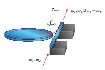
Figure 1: (Color online) Sketch of the studied system (from Ref.Tang ). The microdisk cavity is driven by a pump field and a Stokes field. The nonlinearity of the interaction also generates anti-Stokes field.

In a rotating frame at pump frequency $\omega_{l}$, the Hamiltonian of the system is given by Tang

$$\begin{array}[]{lcl}\displaystyle H=\hbar[\omega_{c}(q)-\omega_{l}]c^{{\dagger}}c+\frac{p^{2}}{2m}+\frac{1}{2}m\omega_{m}^{2}q^{2}\vspace{0.1in}\\ \hskip 21.68121pt+\hbar\frac{L}{c}\tilde{n}_{g}(\omega_{l}\varepsilon_{l}^{2}+\omega_{s}|\varepsilon_{s}|^{2})+i\hbar\sqrt{2\kappa_{e}(q)}\varepsilon_{l}(c^{{\dagger}}-c)\vspace{0.1in}\\ \hskip 21.68121pt+i\hbar\sqrt{2\kappa_{e}(q)}(\varepsilon_{s}e^{-i\delta t}c^{{\dagger}}-\varepsilon^{*}_{s}e^{i\delta t}c).\end{array}$$ (1)

The first term is the energy of the cavity field, whose annihilation (creation) operators are denoted $c(c^{{\dagger}})$. The second and third terms are the energy of the waveguide with mass $m$, frequency $\omega_{m}$, and momentum operator $p$. The fourth term gives the interactions between the waveguide and the incident fields (the pump field and the Stokes field), $L$ is the length of the waveguide, $c$ is the speed of light in vacuum, $\tilde{n}_{g}$ is the group index of the waveguide optical mode Pernice , $\varepsilon_{l}$ and $|\varepsilon_{s}|$ are the amplitudes of the pump field and the Stokes field, respectively, and they are related to their corresponding power $\wp_{l}$ and $\wp_{s}$ by $\varepsilon_{l}=\displaystyle\sqrt{\frac{\wp_{l}}{\hbar\omega_{l}}}$ and $|\varepsilon_{s}|=\displaystyle\sqrt{\frac{\wp_{s}}{\hbar\omega_{s}}}$. The latter two terms describe the coupling of the cavity field to the pump field and the Stokes field, respectively. And $\delta=\omega_{s}-\omega_{l}$ is the detuning between the Stokes field and the pump field. We would study the physical effects by scanning the Stokes laser.

For a small displacement $q$, $\omega_{c}(q)$ and $\kappa_{e}(q)$ can be expanded to the first order of $q$,

$$\begin{array}[]{lcl}\displaystyle\omega_{c}(q)\approx\omega_{c}+q\chi,\vspace{0.2in}\\ \displaystyle\kappa_{e}(q)\approx\kappa_{e}+q\kappa_{om},\end{array}$$ (2)

thus the quantities $\chi$ and $\kappa_{om}$ describe the cavity-waveguide dispersive and reactive coupling strength, respectively. Further, note that the photons in the cavity can leak out of the cavity by an intrinsic damping rate $\kappa_{i}$ of the cavity and by a rate of $\kappa_{e}(q)$ due to the reactive coupling between the waveguide and the cavity. In addition, the velocity of the waveguide is damped at a rate of $\gamma_{m}$. Applying the Heisenberg equation of motion and adding the damping terms, the time evolutions of the expectation values ($\langle q\rangle,\langle p\rangle$, and $\langle c\rangle$) for the system can be expressed as

$$\begin{array}[]{lcl}\displaystyle\langle\dot{q}\rangle=\frac{\langle p\rangle}{m},\vspace{0.2in}\\ \displaystyle\langle\dot{p}\rangle=-m\omega_{m}^{2}\langle q\rangle-\hbar\chi\langle c^{{\dagger}}\rangle\langle c\rangle\displaystyle-2\hbar\frac{\kappa_{om}}{\sqrt{\kappa}}\vspace{0.2in}\\ \hskip 28.90755pt\times\mbox{Im}[(\varepsilon_{l}+\varepsilon^{*}_{s}e^{i\delta t})\langle c\rangle]-\gamma_{m}\langle p\rangle,\vspace{0.2in}\\ \displaystyle\langle\dot{c}\rangle=-[\kappa+\langle q\rangle\kappa_{om}+i(\omega_{c}-\omega_{l}+\langle q\rangle\chi)]\langle c\rangle\vspace{0.2in}\\ \hskip 28.90755pt\displaystyle+\sqrt{\kappa}[1+\langle q\rangle\frac{\kappa_{om}}{\kappa}](\varepsilon_{l}+\varepsilon_{s}e^{-i\delta t}),\end{array}$$ (3)

where we have used the mean field assumption $\langle qc\rangle=\langle q\rangle\langle c\rangle$, expanded $\kappa_{e}(q)$ to the first order of $q$, and assumed $\kappa_{e}\approx\kappa_{i}\approx\kappa/2$, where $\kappa$ is the half-linewidth of the cavity field. It should be noted that the steady-state solution of Eq. (3) contains an infinite number of frequencies. Since the Stokes field $\varepsilon_{s}$ is much weaker than the pump field $\varepsilon_{l}$, the steady-state solution of Eq. (3) can be simplified to first order in $\varepsilon_{s}$ only. We find that in the limit $t\rightarrow\infty$, each $\langle q\rangle$,$\langle p\rangle$, and $\langle c\rangle$ has the form

$$\begin{array}[]{lcl}\langle s\rangle=s_{0}+s_{+}\varepsilon_{s}e^{-i\delta t}+s_{-}\varepsilon^{*}_{s}e^{i\delta t},\end{array}$$ (4)

where $s$ stands for any of the three quantities $q$, $p$, and $c$. Thus the expectation values $(\langle q\rangle,\langle p\rangle$, and $\langle c\rangle$) oscillate at three frequencies ($\omega_{l}$, $\omega_{s}$, and 2$\omega_{l}-\omega_{s}$). Substituting Eq. (4) into Eq. (3), ignoring those terms containing the small quantities $\varepsilon_{s}^{2}$, $\varepsilon_{s}^{*2}$, $|\varepsilon_{s}|^{2}$, and equating coefficients of terms with the same frequency, respectively, we obtain the following results

$$\begin{array}[]{lcl}\displaystyle c_{0}=\frac{A\varepsilon_{l}}{\kappa+q_{0}\kappa_{om}+i\Delta},\vspace{0.1in}\\ q_{0}=\displaystyle-\frac{\hbar}{m\omega_{m}^{2}}[\chi|c_{0}|^{2}+i\frac{\kappa_{om}}{\sqrt{\kappa}}\varepsilon_{l}(c_{0}^{*}-c_{0})],\vspace{.1in}\\ c_{+}=\displaystyle\frac{1}{d(\delta)}[A(BE+FJ)-i\hbar\frac{\kappa_{om}}{\sqrt{\kappa}}c_{0}^{*}BF^{*}],\vspace{.1in}\\ c_{-}=\displaystyle\frac{F^{*}}{d^{*}(\delta)}(-AJ+i\hbar\frac{\kappa_{om}}{\sqrt{\kappa}}c_{0}V),\vspace{0.1in}\\ q_{+}=\displaystyle\frac{B}{d(\delta)}(-AJ^{*}-i\hbar\frac{\kappa_{om}}{\sqrt{\kappa}}c_{0}^{*}V^{*}),\vspace{0.1in}\\ q_{-}=(q_{+})^{*},\end{array}$$ (5)

where

$$\Delta=\omega_{c}-\omega_{l}+\chi q_{0},$$ (6)

$$\begin{array}[]{lcl}d(\delta)=V^{*}(BE+FJ)+BF^{*}J^{*},\end{array}$$ (7)

and $A=\displaystyle\sqrt{\kappa}(1+\frac{\kappa_{om}}{\kappa}q_{0})$, $B=\kappa+q_{0}\kappa_{om}-i(\Delta+\delta)$, $E=m(\omega_{m}^{2}-\delta^{2}-i\gamma_{m}\delta)$, $F=-c_{0}^{*}(\kappa_{om}-i\chi)+\displaystyle\frac{\kappa_{om}}{\sqrt{\kappa}}\varepsilon_{l}$, $J=\chi\hbar c_{0}+i\hbar\displaystyle\frac{\kappa_{om}}{\sqrt{\kappa}}\varepsilon_{l}$, $V=\kappa+q_{0}\kappa_{om}-i(\Delta-\delta)$. The approach used in this paper is similar to our earlier work Sumei2 which dealt with optomechanical systems with dispersive coupling only.

III output fields

To investigate the normal mode splitting of the output fields, we need to calculate their expectation value. It can be obtained by using the input-output relation Walls $\langle c_{out}\rangle=\sqrt{2\kappa_{e}(q)}\langle c\rangle$. If we write $\langle c_{out}\rangle$ as

$$\begin{array}[]{lcl}\langle c_{out}\rangle=c_{l}+\varepsilon_{s}e^{-i\delta t}c_{s}+\varepsilon^{*}_{s}e^{i\delta t}c_{as},\end{array}$$ (8)

where $c_{l}$ is the response at the pump frequency $\omega_{l}$, $c_{s}$ is the response at the Stokes frequency $\omega_{s}$, and $c_{as}$ is the field generated at the new anti-Stokes frequency $2\omega_{l}-\omega_{s}$. Then we have

$$\begin{array}[]{lcl}c_{l}=\displaystyle\sqrt{\kappa}(1+\frac{\kappa_{om}}{\kappa}q_{0})c_{0},\vspace{0.1in}\\ c_{s}=\displaystyle\frac{\kappa_{om}}{\sqrt{\kappa}}q_{+}c_{0}+\sqrt{\kappa}(1+\frac{\kappa_{om}}{\kappa}q_{0})c_{+},\vspace{0.1in}\\ c_{as}=\displaystyle\frac{\kappa_{om}}{\sqrt{\kappa}}q_{-}c_{0}+\sqrt{\kappa}(1+\frac{\kappa_{om}}{\kappa}q_{0})c_{-}.\vspace{0.1in}\\ \end{array}$$ (9)

Furthermore, whether there is normal mode splitting in the output fields is determined by the roots of the denominator $d(\delta)$ of $c_{s}$. Here we examine the roots of $d(\delta)$ given by Eq. (7) numerically.

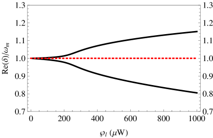
Figure 2: (Color online) The real roots of $d(\delta)$ in the domain Re$(\delta)>0$ as a function of the pump power $\wp_{l}$ for $\kappa_{om}=0$ (dotted curve) and $\kappa_{om}=-2\pi\times 26.6$ MHz/nm (solid curve).

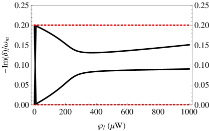
Figure 3: (Color online) Imaginary parts of the roots of $d(\delta)$ as a function of the pump power $\wp_{l}$ for $\kappa_{om}=0$ (dotted curve) and $\kappa_{om}=-2\pi\times 26.6$ MHz/nm (solid curve).

The response of the system is expected to be especially significant if we choose $\omega_{s}$ corresponding to a sideband $\omega_{s}=\omega_{l}\pm\omega_{m}$ or $\omega_{s}=\omega_{l}\pm\Delta$, so we consider the case $\Delta=\omega_{m}$. The other parameters are chosen from a recent experiment focusing on the effect of the reactive force on the waveguide Tang : the wavelength of the laser $\lambda=2\pi c/\omega_{l}=1564.25$ nm, $\chi=2\pi\times 2$ MHz/nm, $m=2$ pg (density of the silicon waveguide, 2.33 g/cm³; length, 10 $\mu$m; width, 300 nm; height, 300 nm), $\kappa=0.2\omega_{m}$, $\omega_{m}=2\pi\times 25.45$ MHz, and the mechanical quality factor $Q=\omega_{m}/\gamma_{m}=5000$. In the following, we work in the stable regime of the system.

Figure 2 shows the variation of the real parts of the roots of $d(\delta)$ in the domain Re$(\delta)>0$ with increasing pump power for no reactive coupling, $\kappa_{om}=0$, and for $\kappa_{om}=-2\pi\times 26.6$ MHz/nm. For $\kappa_{om}=0$, the interaction of the waveguide with the cavity is purely dispersive; the cavity decay rate does not depend on the displacement of the waveguide. In this case, the real parts of the roots of $d(\delta)$ always have two equal values with increasing pump power. Thus there is no splitting because the dispersive coupling is not strong enough. However, for $\kappa_{om}=-2\pi\times 26.6$ MHz/nm, the system has both dispersive and reactive couplings, the cavity decay rate depends on the displacement of the waveguide, and the real parts of the roots of $d(\delta)$ will change from two equal values to two different values with increasing pump power. And the difference between two real parts of the roots of $d(\delta)$ in the domain Re$(\delta)>0$ is increased with increasing pump power. Therefore, the reactive coupling between the waveguide and the cavity can result in normal mode splitting of the output fields, and the peak separation becomes larger with increasing pump power. Figure 3 shows the variation of the imaginary parts of the roots of $d(\delta)$ with increasing pump power for zero reactive coupling $\kappa_{om}=0$ and nonzero reactive coupling $\kappa_{om}=-2\pi\times 26.6$ MHz/nm. For $\kappa_{om}=0$, the imaginary parts of the roots of $d(\delta)$ do not change with increasing pump power. However, for $\kappa_{om}=-2\pi\times 26.6$ MHz, the imaginary parts of the roots of $d(\delta)$ change with increasing pump power. We thus conclude that for the present microdisk resonator coupled to a waveguide the normal mode splitting is solely due to the reactive coupling.

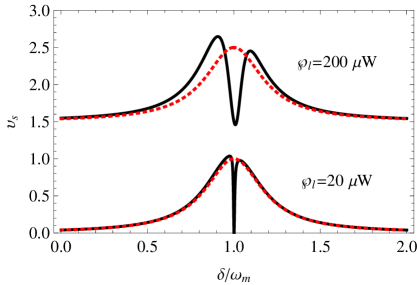
Figure 4: (Color online) The lower two curves show the normalized quadrature $v_{s}$ as a function of the normalized detuning between the Stokes field and the pump field, $\delta/\omega_{m}$ for $\kappa_{om}=0$ (dotted curve) and $\kappa_{om}=-2\pi\times 26.6$ MHz/nm (solid curve) for pump power $\wp_{l}=20$ $\mu$W. The upper two curves give the normalized quadrature $v_{s}$+1.5 for pump power $\wp_{l}=200$ $\mu$W.

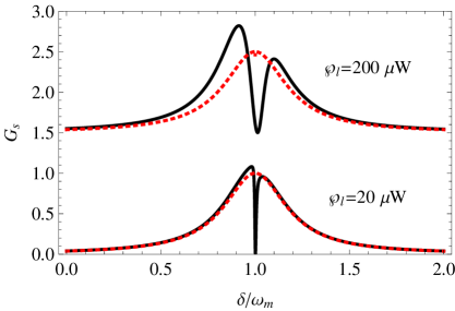
Figure 5: (Color online) The lower two curves show the normalized output power $G_{s}$ as a function of the normalized detuning between the Stokes field and the pump field, $\delta/\omega_{m}$ for $\kappa_{om}=0$ (dotted curve) and $\kappa_{om}=-2\pi\times 26.6$ MHz/nm (solid curve) for pump power $\wp_{l}=20$ $\mu$W. The upper two curves give the normalized output power $G_{s}$+1.5 for pump power $\wp_{l}=200$ $\mu$W.

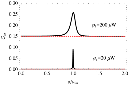
Figure 6: (Color online) The lower two curves show the normalized output power $G_{as}$ as a function of the normalized detuning between the Stokes field and the pump field, $\delta/\omega_{m}$ for $\kappa_{om}=0$ (dotted curve) and $\kappa_{om}=-2\pi\times 26.6$ MHz/nm (solid curve) for pump power $\wp_{l}=20$ $\mu$W. The upper two curves give the normalized output power $G_{as}$+0.15 for pump power $\wp_{l}=200$ $\mu$W.

IV Normal Mode Splitting In Output Fields

We now discuss how the output fields depend on the behavior of the roots of $d(\delta)$. For convenience, we normalize all quantities to the input Stokes power $\wp_{s}$. Assuming that $\varepsilon_{s}$ is real, we express the output power at the Stokes frequency $\omega_{s}$ in terms of the input Stokes power

$$\begin{array}[]{lcl}G_{s}=\displaystyle\frac{\hbar\omega_{s}|\varepsilon_{s}c_{s}|^{2}}{\wp_{s}}=|c_{s}|^{2}.\end{array}$$ (10)

Further, we introduce the two quadratures of the Stokes component of the output fields by $\displaystyle\upsilon_{s}=\frac{c_{s}+c_{s}^{*}}{2}$ and $\displaystyle\tilde{\upsilon}_{s}=\frac{c_{s}-c_{s}^{*}}{2i}$. One can measure either the quadratures of the output by homodyne techniques or the intensity of the output. For brevity, we only show $\upsilon_{s}$ and $G_{s}$ as a function of the normalized detuning between the Stokes field and the pump field $\delta/\omega_{m}$ for this model, without reactive coupling ($\kappa_{om}$=0) and with it ($\kappa_{om}=-2\pi\times 26.6$ MHz/nm), for different pump powers in Figs. 4–5. For $\kappa_{om}$=0, it is found that $\upsilon_{s}$ has a Lorentzian lineshape corresponding to the absorptive behavior. Note that $\upsilon_{s}$ and $G_{s}$ exhibit no splitting when $\kappa_{om}$=0. However, for $\kappa_{om}=-2\pi\times 26.6$ MHz/nm, it is clearly seen that normal mode splitting appears in $\upsilon_{s}$ and $G_{s}$. Therefore reactive coupling can lead to the appearance of normal mode splitting in the output Stokes field. And the peak separation increases with increasing pump power Agarwal . The dip at the line center exhibits power broadening. We also find that the Stokes field can be amplified by the stimulated process. Obviously the maximum gain $G_{s}$ for the Stokes field depends on the system parameters. For a pump power $\wp_{l}=200$ $\mu$W, the maximum gain for the Stokes field is about 1.3.

Note that the nonlinear nature of the reactive coupling generates anti-Stokes radiation. In a similar way, we define a normalized output power at the anti-Stokes frequency $2\omega_{l}-\omega_{s}$ as

$$\begin{array}[]{lcl}G_{as}=\displaystyle\frac{\hbar(2\omega_{l}-\omega_{s})|\varepsilon_{s}c_{as}|^{2}}{\wp_{s}}=|c_{as}|^{2}.\end{array}$$ (11)

The plots of $G_{as}$ versus the normalized detuning between the Stokes field and the pump field $\delta/\omega_{m}$ for this model, without reactive coupling ($\kappa_{om}$=0) and with it ($\kappa_{om}=-2\pi\times 26.6$ MHz/nm), for different pump powers are presented in Fig. 6. We can see that $G_{as}\approx 0$ for $\kappa_{om}$=0. The reason is that the dispersive coupling constant $\chi$ is too small. However, for $\kappa_{om}=-2\pi\times 26.6$ MHz/nm, $G_{as}$ is not equal to zero. This shows that the optomechanical system can generate an anti-Stokes field with frequency $(2\omega_{l}-\omega_{s})$ due to the reactive coupling. For pump power $\wp_{l}=200$ $\mu$W, the maximum gain defined with reference to the input Stokes power for the anti-Stokes field is about 0.1.

V Conclusions

In conclusion, we have observed normal mode splitting of output fields due to reactive coupling between the waveguide and the cavity. Meanwhile, the separation of the peaks increases for larger pump powers. Further, the reactive coupling can also cause four-wave mixing, which creates an anti-Stokes component generated by the optomechanical system.

We gratefully acknowledge support from NSF Grant No. PHYS 0653494.

References

- (1) M. Li, W. H. P. Pernice, and H. X. Tang, Phys. Rev. Lett. 103, 223901 (2009).
- (2) F. Elste, S. M. Girvin, and A. A. Clerk, Phys. Rev. Lett. 102, 207209 (2009).
- (3) M. Li, W. H. P. Pernice, and H. X. Tang, Nat. Photon. 3, 464 (2009).
- (4) M. J. Hartmann and M. B. Plenio, Phys. Rev. Lett. 101, 200503 (2008).
- (5) M. Bhattacharya and P. Meystre, Phys. Rev. Lett. 99, 073601 (2007).
- (6) S. Bose, K. Jacobs, and P. L. Knight, Phys. Rev. A 56, 4175 (1997).
- (7) S. Huang and G. S. Agarwal, New J. Phys. 11, 103044 (2009).
- (8) M. Paternostro, D. Vitali, S. Gigan, M. S. Kim, C. Brukner, J. Eisert, and M. Aspelmeyer, Phys. Rev. Lett. 99, 250401 (2007).
- (9) D. Vitali, S. Gigan, A. Ferreira, H. R. Böhm, P. Tombesi, A. Guerreiro, V. Vedral, A. Zeilinger, and M. Aspelmeyer, Phys. Rev. Lett. 98, 030405 (2007).
- (10) F. Marquardt, J. P. Chen, A. A. Clerk, and S. M. Girvin, Phys. Rev. Lett. 99, 093902 (2007).
- (11) J. M. Dobrindt, I. Wilson-Rae, and T. J. Kippenberg, Phys. Rev. Lett. 101, 263602 (2008).
- (12) S. Gröblacher, K. Hammerer, M. Vanner, and M. Aspelmeyer, Nature (London) 460, 724 (2009).
- (13) S. Huang and G. S. Agarwal, Phys. Rev. A 81, 033830 (2010). [this paper deals exclusively with designs where only dispersive optomechanical coupling occurs.]
- (14) W. H. P. Pernice, M. Li, and H. X. Tang, Opt. Express 17, 1806 (2009).
- (15) D. F. Walls and G. J. Milburn, Quantum Optics (Springer-Verlag, Berlin, 1994).
- (16) G. S. Agarwal and S. Huang, Phys. Rev. A 81, 041803(R) (2010); P. Anisimov and O. Kocharovskaya, J. Mod. Opt. 55, 3159 (2008).