Nonlinear quantum model for atomic Josephson junctions with one and two bosonic species

Abstract

We study atomic Josephson junctions (AJJs) with one and two bosonic species confined by a double-well potential. Proceeding from the second quantized Hamiltonian, we show that it is possible to describe the zero-temperature AJJs microscopic dynamics by means of extended Bose-Hubbard (EBH) models, which include usually-neglected nonlinear terms. Within the mean-field approximation, the Heisenberg equations derived from such two-mode models provide a description of AJJs macroscopic dynamics in terms of ordinary differential equations (ODEs). We discuss the possibility to distinguish the Rabi, Josephson, and Fock regimes, in terms of the macroscopic parameters which appear in the EBH Hamiltonians and, then, in the ODEs. We compare the predictions for the relative populations of the Bose gases atoms in the two wells obtained from the numerical solutions of the two-mode ODEs, with those deriving from the direct numerical integration of the Gross-Pitaevskii equations (GPEs). Our investigations shows that the nonlinear terms of the ODEs are crucial to achieve a good agreement between ODEs and GPEs approaches, and in particular to give quantitative predictions of the self-trapping regime.

1 Introduction

The prediction [1] of Bose-Einstein condensation (BEC) and the experimental achievement of BEC [2] has played a crucial role for theoretical and experimental developments in the physics of ultracold atoms. The study of the atomic counterpart [3, 4, 5, 6, 7] of the Josephson effect which occurs in superconductor-oxide-superconductor junctions [8] - which is an example of macroscopic quantum coherence - represents one of these developments. Albiez et al. [9] have provided the first experimental realization of the atomic Josephson junction (AJJ) previously analyzed theoretically in a certain number of papers [3, 4, 5, 6, 7]. In 2007 Gati et al. [10] reviewed the experiment by Albiez et al. [9] and compared the experimental data with the predictions of a many-body two-mode model [11] and a mean-field description. In the above references the analysis of AJJs physics is carried out in the presence of a single bosonic component. The possibility to tune intra- and inter-species interactions [12, 13] by means of the Feshbach resonance technique makes possible to study of AJJs with two bosonic species trapped together by double-well potentials and to use BECs mixtures as powerful instruments to investigate quantum coherence and nonlinear phenomena, with particular attention to the existence of self-trapped modes and intrinsically localized states.

In the superfluid regime the dynamics of the relative populations and relative phases of the Bose condensed atoms can be described by Josepshon’s two-mode equations, which are ordinary differential equations (ODEs), see for example Refs. [5, 14, 15, 16, 17]. This description is achieved in the presence of a confining double-well potential, with a single bosonic component [5] and also with bosonic mixtures [14, 15, 16, 17, 18]. One of the most interesting aspects of AJJs analysis is to compare the predictions deriving from the ODEs with the ones obtained from the Gross-Pitaevskii equations (GPEs). For single component condensates, Salasnich et al. [6] have shown that a good agreement exists between the results obtained from the GPE and those of the ODEs. Similar agreement was obtained in [7] for AJJs realized with weakly interacting solitons localized in two adjacent wells of an optical lattice. However, the situation may be quite different for multicomponent condensates, due to the interplay of intra- and inter-species interactions which enlarges the number of achievable states (for instance, mixed symmetry states can exist only in the presence of the inter-species interaction) as well as their stability, giving to the system many more dynamical possibilities. Recently it was shown that for the two components case the integration of the ODEs allows to predict the analogous of the macroscopic quantum self-trapping phenomenon observed in AJJs with one bosonic component [15, 17]. This phenomenon has been discussed for a two-components nonlinear Schrödinger model with a double-well potential by Wang and co-workers [19]. More recently, a comparison between the reduced ODEs system and the full GPE dynamics was performed, showing that, for various conditions, a good agreement exists between the two kinds of predictions [17].

The aim of the present work is to analyze how the accuracy of the two-mode approximation can be improved by taking into account the usually-neglected nonlinear terms. These terms derive from the overlaps between wave functions localized in different wells. Both for single component and for two components AJJs - introduced in the second section - we proceed from a full second quantized description of the system. In Sec. III we describe the system by the extended Bose-Hubbard (EBH) Hamiltonian. In the single component case, the EBH Hamiltonian is the two-sites restriction of the Hamiltonian considered in Refs. [20, 21] to analyze bosons loaded in one dimensional optical lattices. In the two species case, the EBH Hamiltonian is the extended version of the one considered by Kuklov and Svistunov in Ref. [22] to study the counterflow superfluidity of two-species ultracold atoms. We note that the study of the two components bosonic system proceeding from a pure quantum approach is a subject of wide interest. In fact, this topic is dealt with in certain regions of the phase space in Ref. [23] and in the case of hardcore bosons as discussed in Ref. [24].

The EBH Hamiltonian sustains the dynamics of the single-particle operators via the Heisenberg equations of motion [25, 26]. By performing the mean-field approximation on the single-particle operators of each component, the improved ODEs are achieved. In the third section we also discuss how it is possible to distinguish the Rabi regime, the Josephson regime, and the Fock regime. This analysis is carried out in terms of the macroscopic parameters involved in the EBH Hamiltonians and, then, at the right hand sides of the improved ODEs as discussed for single AJJs in Ref. [27]. In Sec. IV we write down the GPEs for the one and the two components AJJs. Here we compare the results obtained by numerically integrating the GPEs with the predictions obtained by numerically solving the improved ODEs. Moreover, in the fourth section we plot the phase-plane portraits of the dynamical variables fractional imbalance-relative phase. Finally, in Sec. V we draw our conclusions.

2 The system

We consider two interacting dilute and ultracold Bose gases denoted below by $1$ and $2$. We suppose that the two gases are confined in a double-well trap produced, for example, by a far off-resonance laser barrier that separates each trapped condensate in two parts, L (left) and R (right). We assume, moreover, that the two condensates interact with each other and that the trapping potential $V_{trap}({\bf r})$ for both components is taken to be the superposition of a strong harmonic confinement in the radial ($x$-$y$) plane and of a double-well (DW) potential in the axial ($z$) direction. We model the trapping potential as:

$$V_{trap}({\bf r})=\frac{m_{i}\omega_{i}^{2}}{2}(x^{2}+y^{2})+V_{DW}(z)\;,$$ (1)

where $m_{i}$ is the mass of the $i$th component. For simplicity we take $\omega_{1}=\omega_{2}\equiv\omega$. For symmetric configurations in the $z$ direction, we take - for the $i$th species - the double-well in Eq. (1) as

$$V_{DW}(z)=V_{L}(z)+V_{R}(z)$$

$$V_{L}(z)=-V_{0}\bigg{[}Sech^{2}(\frac{z+z_{0}}{b})\bigg{]}$$

$$V_{R}(z)=-V_{0}\bigg{[}Sech^{2}(\frac{z-z_{0}}{b})\bigg{]}$$

$$V_{0}=\hbar\omega_{i}\big{[}1+Sech^{2}(\frac{2z_{0}}{b})\big{]}^{-1}\;,$$

that is the combination of two Pöschl-Teller (PT) potentials, $V_{L}(z)$ and $V_{R}(z)$, centered at the points $-z_{0}$ and $z_{0}$, and separated by a potential barrier which may be changed by varying $b$ (see Fig. 1). We use PT potentials only for the benefit of improving accuracy in our numerical GPEs calculations (see the fourth section), taking advantage of the integrability of the underlying linear system. We remark, however, that our results apply to a generic double-well potential. Eigenvalues and eigenfuctions of the Pöschl-Teller potential for a single well are known analytically. The wave functions of the ground state of $V_{\alpha}(z)$ ($\alpha=L,R$), centered around $-z_{0}$ ($+z_{0}$) are [28] :

$$\phi_{(\alpha,i,PT)}(z)=A\big{[}1-Tanh^{2}(\frac{z\pm z_{0}}{b})\big{]}^{B_{i}/2}$$

$$B_{i}=-\frac{1}{2}+\sqrt{\frac{2m_{i}V_{0}b^{2}}{\hbar^{2}}+\frac{1}{4}}\;.$$ (3)

The constant $A$, in Eq. (2), ensures the normalization of the wave function in each well.

Figure 1: The double-well potential (2) as a function of $z$ for $z_{0}=3$ and different values of $b$. The dot-dashed line corresponds to $b=0.7$, the continuous line corresponds to $b=1$, and the dashed line corresponds to $b=1.3$. Lengths are measured in units of $\displaystyle{a_{\bot,i}=\sqrt{\frac{\hbar}{m_{i}\omega}}}$ and energies in units of $\hbar\omega$ .

3 The second quantization Hamiltonian

To describe our system at zero-temperature, we proceed from the second quantized Hamiltonian, which reads

$$\hat{H} = \sum_{i=1,2}\int d^{3}{\bf r}\,\hat{\Psi}^{\dagger}_{i}({\bf r})\bigg{(}-\frac{\hbar^{2}}{2m_{i}}\nabla^{2}+V_{trap}({\bf r})\bigg{)}\hat{\Psi}_{i}({\bf r})$$ (4)

$$+ \sum_{i=1,2}\frac{g_{i}}{2}\int d^{3}{\bf r}\hat{\Psi}^{\dagger}_{i}({\bf r})\hat{\Psi}^{\dagger}_{i}({\bf r})\hat{\Psi}_{i}({\bf r})\hat{\Psi}_{i}({\bf r})$$

$$+ g_{12}\int d^{3}{\bf r}\hat{\Psi}^{\dagger}_{1}({\bf r})\hat{\Psi}^{\dagger}_{2}({\bf r})\hat{\Psi}_{2}({\bf r})\hat{\Psi}_{1}({\bf r})\;,$$

where $V_{trap}({\bf r})$ is the potential (1). The coupling constants $g_{i}$ and $g_{12}$ are the intra- and inter-species atom-atom interaction strengths, respectively. These constants are given by

$$g_{i}=\frac{4\pi\hbar^{2}a_{i}}{m_{i}}\;,$$ (5)

$$g_{12}=\frac{2\pi\hbar^{2}a_{12}}{m_{r}}\;,$$ (6)

where the reduced mass $m_{r}$ is equal to $m_{1}m_{2}/(m_{1}+m_{2})$. Eqs. (5) and (6) relate the two coupling constants to the respective s-wave scattering lengths, $a_{i}$ and $a_{12}$. In the following, we shall consider both $g_{i}$ and $g_{12}$ as free parameters, due to the possibility of changing the s-wave scattering lengths $a_{i}$ and $a_{12}$ by the technique of Feshbach resonances. In the following, we will neglect the mass difference between the two bosonic components of the mixture, as for example in Ref. [13], and assume that $m_{1}=m_{2}\equiv m$. In Eq. (4), the field $\hat{\Psi}_{i}({\bf r})$ ($\hat{\Psi}^{\dagger}_{i}({\bf r})$) destroys (creates) a boson of the $i$th species at the point ${\bf r}$, and obeys the usual bosonic commutation relations. We expand the field operator $\hat{\Psi}_{i}({\bf r})$ in terms of operators $\hat{a}_{\alpha,i}$ ($\hat{a}^{\dagger}_{\alpha,i})$ - destroying (creating) a boson of the $i$th species in the well $\alpha=L,R$ - according to:

$$\hat{\Psi}_{i}({\bf r})=\sum_{\alpha=L,R}\Phi_{\alpha,i}({\bf r})\hat{a}_{\alpha,i}\;,$$ (7)

where $\hat{a}$’s and $\hat{a}^{\dagger}$’s satisfy the usual boson commutation relations and the functions $\Phi_{\alpha,i}$ form an orthonormal set. Due to the form (1) of the trapping potential, $\Phi_{\alpha,i}({\bf r})$ can be decomposed as

$$\Phi_{\alpha,i}({\bf r})=w_{i}(x)w_{i}(y)\phi_{\alpha,i}(z)\;,$$ (8)

where $w_{i}(x)$ and $w_{i}(y)$ are the ground state wave functions of the harmonic oscillator potentials $\displaystyle{m_{i}\omega_{i}^{2}x^{2}/2}$ and $\displaystyle{m_{i}\omega_{i}^{2}y^{2}/2}$, respectively. The functions $\phi_{L,i}(z)$ and $\phi_{R,i}(z)$ at right hand side of Eq. (8) are two functions well localized in the left and right well, respectively. These functions are real and orthonormal. The functions $\phi_{L,i}(z)$ and $\phi_{R,i}(z)$ can be determined following the same perturbative approach as in Ref. [17]. Under the same conditions, these functions may be written in terms of the $\phi_{(L,i,PT)}(z)$ and $\phi_{(R,i,PT)}(z)$ of Eq. (2) as:

$$\phi_{L,i}(z)=\frac{1}{2}\bigg{[}(\frac{1}{\sqrt{1+s}}+\frac{1}{\sqrt{1-s}})\phi_{(L,i,PT)}(z)+(\frac{1}{\sqrt{1+s}}-\frac{1}{\sqrt{1-s}})\phi_{(R,i,PT)}(z)\bigg{]}$$

$$\phi_{R,i}(z)=\frac{1}{2}\bigg{[}(\frac{1}{\sqrt{1+s}}-\frac{1}{\sqrt{1-s}})\phi_{(L,i,PT)}(z)+(\frac{1}{\sqrt{1+s}}+\frac{1}{\sqrt{1-s}})\phi_{(R,i,PT)}(z)\bigg{]}\ \;,$$

where $s=\int_{-\infty}^{+\infty}dz\,\phi_{(L,i,PT)}(z)\phi_{(R,i,PT)}(z)$.

3.1 AJJs with a single bosonic species

Let us start our analysis by considering the presence of a single bosonic component. In this case, the inter-species coupling constant (6) is equal to zero. We use the field operator expansion (8) in the second quantized Hamiltonian (4). The AJJs microscopic dynamics is controlled by the EBH Hamiltonian [20, 25, 26]. The EBH model, by omitting the species index $i$, is described by the Hamiltonian

$$\hat{H}_{EBH} = E_{L}^{0}\hat{a}_{L}^{\dagger}\hat{a}_{L}+E_{R}^{0}\hat{a}_{R}^{\dagger}\hat{a}_{R}+\frac{U_{L}}{2}\hat{a}_{L}^{\dagger}\hat{a}_{L}^{\dagger}\hat{a}_{L}\hat{a}_{L}$$

$$+ \frac{U_{R}}{2}\hat{a}_{R}^{\dagger}\hat{a}_{R}^{\dagger}\hat{a}_{R}\hat{a}_{R}-K\big{(}\hat{a}_{L}^{\dagger}\hat{a}_{R}+\hat{a}_{R}^{\dagger}\hat{a}_{L}\big{)}$$

$$+ K_{c}\big{(}\hat{a}_{L}^{\dagger}\hat{n}_{L}\hat{a}_{R}+\hat{a}_{L}^{\dagger}\hat{n}_{R}\hat{a}_{R}+\hat{a}^{\dagger}_{R}\hat{n}_{L}\hat{a}_{L}+\hat{a}_{R}^{\dagger}\hat{n}_{R}\hat{a}_{L}\big{)}$$

$$+ V\hat{a}_{L}^{\dagger}\hat{a}_{R}^{\dagger}\hat{a}_{L}\hat{a}_{R}+K_{p}\big{(}\hat{a}_{L}^{\dagger}\hat{a}_{L}^{\dagger}\hat{a}_{R}\hat{a}_{R}+\hat{a}_{R}^{\dagger}\hat{a}_{R}^{\dagger}\hat{a}_{L}\hat{a}_{L}\big{)}\;.$$

Here $\hat{n}_{\alpha}=\hat{a}^{\dagger}_{\alpha}\hat{a}_{\alpha}$ is the number of particles in the $\alpha$th well. $E_{\alpha}^{0}$ are the energies of the two wells, $U_{\alpha}>0$ are the boson-boson repulsive interaction amplitudes, and $K$ is the tunnel matrix element, which is the Rabi oscillation energy in the case of a model with $U_{\alpha}$ equal to zero. The parameter $K_{c}$ is the induced collisionally hopping amplitude, $V$ is the density-density bosonic interaction amplitude, and $K_{p}$ describes the pair bosonic hopping [20]. By using the decomposition (8) and the explicit form of $w(x)$ and $w(y)$, the macroscopic parameters (3.1) may be shown to be related to the intra-species coupling constant (5) and to the other microscopic parameters (the mass and the frequency of the harmonic trap) by the formulas

$$E_{\alpha}^{0}=\int dz\bigg{[}\frac{\hbar^{2}}{2m}(\frac{d\phi_{\alpha}}{dz})^{2}+(V_{DW}+\frac{\hbar^{2}}{2ma^{2}_{\bot}}+\frac{m\omega^{2}a^{2}_{\bot}}{2})(\phi^{\alpha})^{2}\bigg{]}$$

$$U_{\alpha}=\tilde{g}\int_{-\infty}^{+\infty}{dz\,({\phi_{\alpha}}(z))^{4}}$$

$$K=-\int dz\,\bigg{[}\frac{\hbar^{2}}{2m}\frac{d\phi_{L}}{dz}\frac{d\phi_{R}}{dz}+V_{DW}(z)\phi_{L}\phi_{R}\bigg{]}$$

$$K_{c}=\tilde{g}\int_{-\infty}^{+\infty}{dz\,({\phi_{\alpha}}(z))^{3}\,\phi_{\beta}(z)}$$

$$V=2\tilde{g}\int_{-\infty}^{+\infty}{dz\,({\phi_{\alpha}}(z))^{2}\,({\phi_{\beta}}(z))^{2}}$$

$$K_{p}=\frac{V}{4}\;,$$ (11)

where $\tilde{g}=\displaystyle{\frac{g}{2\pi a^{2}_{\bot}}}$. We observe that the first two lines of Hamiltonian (3.1) involve only the overlaps between $\phi_{\alpha}$’s localized in the same well, see [5]. The third and fourth lines of the Hamiltonian (3.1) include also the overlaps between $\phi_{\alpha}$’s localized in different wells, see [27]. Proceeding from the Hamiltonian (3.1), we write down criteria to individuate different oscillations regimes sustained by the AJJs dynamics. To this end, as discussed in Refs. [4, 27], we express the Hamiltonian (3.1) in terms of the following operators:

$$\hat{J}_{x}=\frac{1}{2}(\hat{a}^{\dagger}_{L}\hat{a}_{L}-\hat{a}^{\dagger}_{R}\hat{a}_{R})$$ (12)

$$\hat{J}_{y}=\frac{i}{2}(\hat{a}^{\dagger}_{L}\hat{a}_{R}-\hat{a}^{\dagger}_{R}\hat{a}_{L})$$

$$\hat{J}_{z}=\frac{1}{2}(\hat{a}^{\dagger}_{L}\hat{a}_{R}+\hat{a}^{\dagger}_{R}\hat{a}_{L})\;,$$

and the $SU(2)$ algebra invariant $\hat{J}^{2}=(\hat{N}/2)(\hat{N}/2+1)$, with $\hat{N}$ being equal to $\hat{n}_{L}+\hat{n}_{R}$ [29].

We assume that the two potential wells are symmetric, $E^{0}_{L}=E^{0}_{R}\equiv E$ and $U_{L}=U_{R}\equiv U$. Neglecting constant terms, and using the fact that $N\gg 1$, we get

$$\hat{H}=(U-V)\hat{J}^{2}_{x}-2\,(K-K_{c}\,N)\hat{J}_{z}+V\hat{J}^{2}_{z}\;.$$ (13)

Here, if the condition $(U-V)\gg V$ is verified, we can consider only the terms in $\hat{J}^{2}_{x}$ and $\hat{J}_{z}$. Then by defining the parameter $R$ as

$$R=\frac{(U-V)\,N}{(K-K_{c}N)}\;$$ (14)

we are able (see Ref. [4]) to distinguish the three following regimes

• Rabi: $R\ll 1$;

• Josephson: $1\ll R\ll N^{2}$;

• Fock: $N^{2}\ll R$.

In the Rabi regime the bosons are in a coherent state and oscillate with a frequency given simply by the energy difference between the ground state and the first excited state associated to the double-well potential. In the Josephson regime the bosons are in a coherent state and oscillate with a frequency which depends on the parameters $U$, $K_{c}$, and $V$. Moreover, if the interaction strength is sufficiently large the self-trapping takes place. In the Fock regime the bosons are in a Fock state characterized by the suppression of number fluctuations. Now, we observe that the Hamiltonian (3.1) can be viewed as the two sites restriction of the Hamiltonian considered in Refs. [20, 21] within the study of bosons loaded in one dimensional optical lattices. In particular, in Ref. [20] it is shown that within the Fock regime two regions open up. To this end we denote by $\Delta$ the energetic gap between the Fock state with $N_{0}$ bosons per well and the Fock state with $(N_{0}+1)$ per well [20]

$$\Delta=2(E+U\,N_{0})\;.$$ (15)

Then, when

$$|4\Delta-(2\,N_{0}+1)\,V|>V$$ (16)

we have a pure Mott insulating phase (PMI), driven by the density-density on-site interaction. When

$$|4\Delta-(2\,N_{0}+1)\,V|<V$$ (17)

we have a Density-Wave Mott insulating (DWMI) regime, driven by the nearest-neighbors interaction [20]. Note that the DWMI phase is characterized by number fluctuations suppression as well.

At this point, we remark that we are interested in determining the fully coherent dynamical oscillations of population of the Bose condensed atoms between the left and right wells. Then, we proceed from the Heisenberg equations of motion for the model Hamiltonian (3.1). These equations of motion control the temporal evolution of $\hat{a}_{\alpha}$. We observe that in the superfluid regime the system is in a coherent state and the following mean-field approximation [25]

$$\langle\hat{a}_{\alpha}\rangle=\sqrt{N_{\alpha}}\exp(i\theta_{\alpha})$$

$$\langle\hat{n}_{\alpha}\rangle=N_{\alpha}\;$$ (18)

can be performed. The averages involved in Eq. (3.1) are evaluated with respect to the coherent state. Under the assumption of symmetric wells and by inserting the mean-field approximation (3.1) into the aforementioned Heisenberg equations of motion, we get

$$\dot{z}(t)=-\frac{2(K-K_{c}N)}{\hbar}\,\sqrt{1-z^{2}(t)}\,\sin\theta(t)$$ (19)

$$+ \frac{VN}{2\hbar}(1-z^{2}(t))\sin 2\theta(t)$$

$$\dot{\theta}(t)=\frac{U-V}{\hbar}Nz(t)+\frac{2(K-K_{c}N)}{\hbar}\,\frac{z(t)\cos\theta(t)}{\sqrt{1-z^{2}(t)}}$$

$$- \frac{VN}{2\hbar}\,z(t)\cos 2\theta(t)\;,$$

where $N=N_{L}+N_{R}$ is the total number of bosons, and $z=(N_{L}-N_{R})/N$ and $\theta=\theta_{R}-\theta_{L}$ are, respectively, the fractional imbalance and the relative phase.

3.2 AJJs with two bosonic species

In this subsection we shall consider AJJs in the presence of two interacting bosonic components. In this case both the coupling constants (5) and (6) are finite, and the two mode EBH model is described by the Hamiltonian

$$\hat{H}=\sum_{i=1,2}\hat{H}_{(EBH,i)}+\hat{H}_{12}\;.$$ (20)

The Hamiltonian $\hat{H}_{(EBH,i)}$ is the single component Hamiltonian (3.1) written in terms of the operators $\hat{a}_{\alpha,i}$ and $\hat{a}^{\dagger}_{\alpha,i}$. The parameters $E^{0}_{\alpha}$, $U_{\alpha}$, $K$, $K_{c}$, $V$, $K_{p}$, and the function $\phi_{\alpha}$ will read $E^{0}_{\alpha,i}$, $U_{\alpha,i}$, $K_{i}$, $K_{c,i}$, $V_{i}$, $K_{p,i}$, and $\phi_{\alpha,i}$, respectively. The microscopic quantities referred to a single bosonic component will be modified according to the same prescription. Under the hypothesis of symmetric wells, the coupling Hamiltonian $\hat{H}_{12}$ reads:

$$\hat{H}_{12} = U_{12}\big{(}\hat{a}^{\dagger}_{L,1}\hat{a}^{\dagger}_{L,2}\hat{a}_{L,1}\hat{a}_{L,2}+\hat{a}^{\dagger}_{R,1}\hat{a}^{\dagger}_{R,2}\hat{a}_{R,1}\hat{a}_{R,2}\big{)}$$ (21)

$$+ V_{12}\big{(}\hat{a}^{\dagger}_{L,1}\hat{a}^{\dagger}_{R,2}\hat{a}_{L,1}\hat{a}_{R,2}+\hat{a}^{\dagger}_{L,2}\hat{a}^{\dagger}_{R,1}\hat{a}_{L,2}\hat{a}_{R,1}\big{)}$$

$$+ K_{p,12}\big{(}\hat{a}^{\dagger}_{L,1}\hat{a}^{\dagger}_{L,2}\hat{a}_{R,2}\hat{a}_{R,1}+\hat{a}^{\dagger}_{R,1}\hat{a}^{\dagger}_{R,2}\hat{a}_{L,2}\hat{a}_{L,1}$$

$$+ \hat{a}^{\dagger}_{L,1}\hat{a}^{\dagger}_{R,2}\hat{a}_{L,2}\hat{a}_{R,1}+\hat{a}^{\dagger}_{R,1}\hat{a}^{\dagger}_{L,2}\hat{a}_{R,2}\hat{a}_{L,1}\big{)}$$

$$+ K_{c,12}\big{(}\hat{a}^{\dagger}_{L,1}\hat{n}_{L,2}\hat{a}_{R,1}+\hat{a}^{\dagger}_{R,1}\hat{n}_{L,2}\hat{a}_{L,1}$$

$$+ \hat{a}^{\dagger}_{L,2}\hat{n}_{L,1}\hat{a}_{R,2}+\hat{a}^{\dagger}_{R,2}\hat{n}_{L,1}\hat{a}_{L,2}$$

$$+ \hat{a}^{\dagger}_{L,2}\hat{n}_{R,1}\hat{a}_{R,2}+\hat{a}^{\dagger}_{R,2}\hat{n}_{R,1}\hat{a}_{L,2}$$

$$+ \hat{a}^{\dagger}_{L,1}\hat{n}_{R,2}\hat{a}_{R,1}+\hat{a}^{\dagger}_{R,1}\hat{n}_{R,2}\hat{a}_{L,1}\big{)}\;.$$

In Eq. (21), $U_{12}$ is the inter-species interaction amplitude between bosons localized in the same well, and $V_{12}$ is the inter-species interaction amplitude between bosons localized in different wells. The quantity $K_{p,12}$ is the inter-species pair hopping (hopping of particle-particle or hole-hole pair made up of bosons of different species); $K_{c,12}$ is the amplitude of the inter-species collisionally induced hopping. By using the decomposition (8) and the explicit form of $w_{i}(x)$ and $w_{i}(y)$, the aforementioned parameters are shown to be related to the inter-species coupling constant (6) by:

$$U_{12}=\tilde{g}_{12}\int_{-\infty}^{+\infty}{dz\,({\phi_{\alpha,i}(z)})^{2}({\phi_{\alpha,j}(z)})^{2}}$$

$$V_{12}=\tilde{g}_{12}\int_{-\infty}^{+\infty}{dz\,({\phi_{\alpha,i}(z)})^{2}(\phi_{\beta,j}(z)})^{2}$$

$$K_{c,12}=\tilde{g}_{12}\int_{-\infty}^{+\infty}\,dz\,(\phi_{\alpha,i}(z))^{3}(\phi_{\beta,j}(z))$$

$$K_{p,12}=V_{12}\;,$$ (22)

where $\displaystyle{\tilde{g}_{12}=\frac{g_{12}}{\pi(a^{2}_{\bot,1}+a^{2}_{\bot,2})}}$. Note that we are considering both the overlaps between $\phi_{\alpha}$’s localized in the same well ($U_{\alpha,i}$ and $U_{12}$) - that are the only terms taken into account in Ref. [17] - and the overlaps between $\phi_{\alpha}$’s localized in different wells ($V_{12}$, $K_{p,12}$, $K_{c,12}$). We observe that, in general, due to the presence of the parameters (3.2) the identification of different oscillation regimes proceeding from the Hamiltonian (20) is not immediate as for single component AJJs. Nevertheless, under certain conditions we are able to write down criteria to select the different regimes sustained by the two components AJJs dynamics. First, let us focus on the case in which only the overlaps between $\phi_{\alpha}$’s localized in the same well are considered. If certain relations exist between the intra- and the inter-species interactions amplitudes, we can recognize the two-species corresponding of the Rabi, Josephson and Fock regimes discussed in the case of single component AJJs. For each component $i$, we define the quantity $\gamma_{i}$ as

$$\gamma_{i}=\frac{U_{i}N_{i}}{K_{i}}\;.$$ (23)

We recognize the following ”weak-coupled” Rabi, Josephson, and Fock regimes

• Rabi: $\gamma_{i}\ll 1$, $|U_{12}|\simeq U_{i}$;

• Josephson: $1\ll\gamma_{i}\ll N_{i}^{2}$, $|U_{12}|\leq U_{i}$;

• Fock: $N_{i}^{2}\ll\gamma_{i}$.

In the Josephson regime, even if the intra-species interaction is not strong enough to ensure self-trapping by itself, self-trapping occurs when the inter-species interaction strength exceeds a crossover value. In the Fock regime the net number of atoms in the transport is suppressed. However, with repulsive inter-species interaction the so-called counterflow survives [22]. This means that the currents of the two species are equal in absolute values and are in opposite directions. This conductive regime is named super(counter)fluid phase (SCF). As discussed in Ref. [22], the system supports the SCF phase of the two components when

$$U_{1}+U_{2}-2\,U_{12}\gg 1\;.$$ (24)

When the condition

$$U_{1}+U_{2}=2\,U_{12}$$ (25)

is met, a phase separation (PS) is observed in the system and the system can be viewed as composed by two totally independent Bose gases confined in the double-well potential. On a physical level, this phase separation means that one bosonic component will occupy the left well and the other the right well. If the inter-species interaction is attractive and the hypothesis $N_{1}=N_{2}\equiv N$ is verified, then, when

$$U_{1}+U_{2}-2\,|U_{12}|\gg 1$$ (26)

a superfluid phase, in which the superfluid consists of pairs of bosons, is supported by the system. This phase is named superfluid paired phase [31].

So far we have neglected the role played by the terms deriving from the overlaps between $\phi_{\alpha}$’s localized in different wells. The presence of these terms makes the scenario more complicated. However, also in this situation, under certain conditions, it is possible to achieve a classification of the oscillations regimes. To this end, as discussed for the single component case, we express the Hamiltonian (20) in terms of the operators $\hat{J}_{x,i}$, $\hat{J}_{y,i}$, $\hat{J}_{z,i}$ defined in Eq. (12) and the $SU(2)$ algebra invariant $\hat{J}_{i}^{2}=(\hat{N}_{i}/2)(\hat{N}_{i}/2+1)$, with $\hat{N}_{i}$ being equal to $\hat{n}_{L,i}+\hat{n}_{R,i}$. Since we are assuming symmetric potential wells, we can write that $E^{0}_{L,i}=E^{0}_{R,i}\equiv E_{i}$, $U_{L,i}=U_{R,i}\equiv U_{i}$. Neglecting constant terms, and using the fact that $N_{i}\gg 1$, we get

$$\hat{H}=(U_{i}-V_{i})\hat{J}^{2}_{x,i}-2\,(K-K_{c,i}\,N_{i}-K_{c,12}\,N_{j})\hat{J}_{z,i}$$

$$+ V_{i}\hat{J}^{2}_{z,i}+4\big{(}(U_{12}-V_{12})\hat{J}_{x,1}\hat{J}_{x,2}+V_{12}\hat{J}_{z,1}\hat{J}_{z,2}\big{)}$$

$$+ U_{12}(\hat{n}_{L,1}\hat{n}_{R,2}+\hat{n}_{R,1}\hat{n}_{L,2})+V_{12}(\hat{n}_{L,1}\hat{n}_{L,2}+\hat{n}_{R,1}\hat{n}_{R,2})\;.$$

Again, if $(U_{i}-V_{i})\gg V_{i},V_{12}$, and $(U_{12}-V_{12})\gg V_{i},V_{12}$, we can consider only the terms in $\hat{J}^{2}_{x,i}$, $\hat{J}_{z,i}$, and $\hat{J}_{x,1}\hat{J}_{x,2}$. We will assume also that $N_{1}=N_{2}\equiv N$, $U_{1}=U_{2}\equiv U$, $V_{1}=V_{2}\equiv V$, and $K_{c,1}=K_{c,2}\equiv K_{c}$, and that the initial conditions are the same for both the components. In analogy to the case of a single component AJJ, we define the parameter $\tilde{R}$ as

$$\tilde{R}=\frac{\big{(}(U-V)+4(U_{12}-V_{12})\big{)}\,N}{\big{(}K-(K_{c}+K_{c,12})N\big{)}}\;.$$ (28)

Again, we are able to distinguish the three regimes:

• Rabi: $\tilde{R}\ll 1$;

• Josephson: $1\ll\tilde{R}\ll N^{2}$;

• Fock: $N^{2}\ll\tilde{R}$.

At this point, we remark that we are interested in determining the fully coherent dynamical oscillations of population of the two bosonic components between the left and right wells. Then, we proceed from the Heinseberg equations of motion for the model Hamiltonian (20). These equations of motion control the temporal evolution of $\hat{a}_{\alpha,i}$. Again, by inserting the mean-field approximation valid in the superfluid regime - $\langle\hat{a}_{\alpha,i}\rangle=\sqrt{N_{\alpha,i}}\exp(i\theta_{\alpha,i})$, $\langle\hat{n}_{\alpha,i}\rangle=N_{\alpha,i}$ - into the aforementioned Heisenberg equations of motion, one gets the coupled differential equations for the fractional imbalance $z_{i}=(N_{L,i}-N_{R,i})/N_{i}$ and relative phase $\theta_{i}=\theta_{R,i}-\theta_{L,i}$ of the two species:

$$\dot{z}_{i}(t) = -\frac{2(K_{i}-K_{c,i}N_{i})}{\hbar}\,\sqrt{1-z_{i}^{2}(t)}\,\sin\theta_{i}(t)$$

$$+ \frac{V_{i}N_{i}}{2\hbar}(1-z_{i}^{2}(t))\sin 2\theta_{i}(t)$$

$$+ \frac{2}{\hbar}(V_{12}\sqrt{1-z_{j}^{2}(t)}\,\cos\theta_{j}(t)$$

$$+ K_{c,12})N_{j}\sqrt{1-z_{i}^{2}(t)}\,\sin\theta_{i}(t)$$

$$\dot{\theta}_{i}(t) = \frac{U_{i}-V_{i}}{\hbar}N_{i}z_{i}(t)+\frac{2(K_{i}-K_{c,i}N_{i})}{\hbar}\,\frac{z_{i}(t)\cos\theta_{i}(t)}{\sqrt{1-z_{i}^{2}(t)}}$$

$$- \frac{V_{i}N_{i}}{2\hbar}\,z_{i}(t)\cos 2\theta_{i}(t)+\frac{U_{12}-V_{12}}{\hbar}N_{j}z_{j}(t)$$

$$- \frac{2}{\hbar}(V_{12}\sqrt{1-z_{j}^{2}(t)}\,\cos\theta_{j}(t)$$

$$+ K_{c,12})N_{j}\frac{z_{i}(t)\cos\theta_{i}(t)}{\sqrt{1-z_{i}^{2}(t)}}\;.$$

4 Gross-Pitaevskii equations predictions: comparison with ordinary differential equations results

So far we have discussed how AJJs dynamics can be described by means of the ODEs, i.e. Eqs. (19) and (3.2). We know that AJJs dynamics can be analyzed, in the mean-field approximation, in terms of partial differential equations, i.e. the GPEs. This description can be achieved proceeding from the Heisenberg motion equations for the field operators $\hat{\Psi}_{i}({\bf r},t)$, ($i=1,2$), associated to the Hamiltonian (4), that is

$$i\hbar\partial_{t}\hat{\Psi}_{i}=[\hat{\Psi}_{i},\hat{H}]\;.$$ (30)

The average - denoted by $\langle...\rangle$ - of both sides of Eq. (30) evaluated with respect to the coherent state, provides the two coupled GPEs

$$i\hbar\frac{\partial\Psi_{i}}{\partial t}=-\frac{\hbar^{2}}{2m_{i}}\nabla^{2}\Psi_{i}+[V_{trap}({\bf r})+g_{i}|\Psi_{i}|^{2}+g_{ij}|\Psi_{j}|^{2}]\Psi_{i}\;.$$ (31)

The macroscopic wave functions $\Psi_{i}({\bf r},t)=\langle\hat{\Psi}_{i}({\bf r},t)\rangle$ of interacting BECs in the trapping potential $V_{trap}({\bf r})$ at zero-temperature satisfy Eq. (31). The wave function $\Psi_{i}({\bf r},t)$ is subject to the normalization condition

$$\int d^{3}{\bf r}\,|\Psi_{i}({\bf r},t)|^{2}=N_{i}\;.$$ (32)

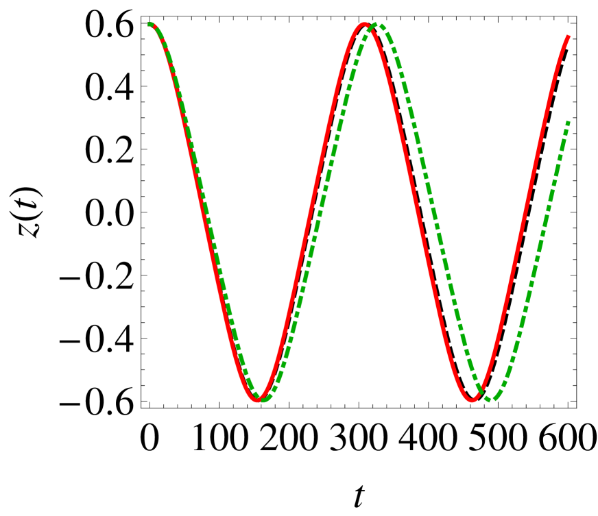
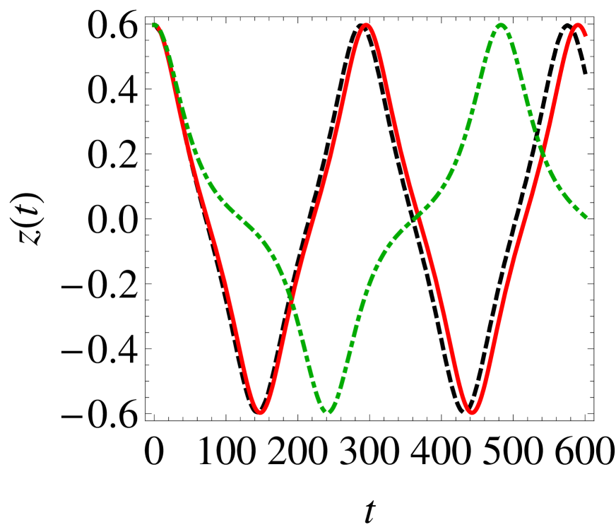
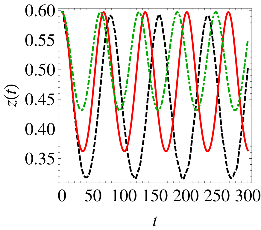
Figure 2: Fractional imbalance $z(t)$ vs. time for single component atomic Josephson junctions. The parameters of the double-well potential (2) are chosen to be $b=1$ and $z_{0}=3$. The dashed line represents data from the integration of GPE (37), the continuous line represents data from the integration of ODEs (19), and the dot-dashed one represents data from the integration ODEs (19) with $K_{c}=V=0$. We have set $N=200$ and $K=4.955\times 10^{-3}$. We have used the initial conditions $z(0)=0.6$ and $\theta(0)=0$. In the top panels (from left to right): $U=0.05\,K$, $K_{c}=-1.842\times 10^{-6}$, $V=2.268\times 10^{-7}$; $U=0.1\,K$, $K_{c}=-3.684\times 10^{-6}$, $V=4.535\times 10^{-7}$. In the bottom panels (from left to right): $U=0.2\,K$, $K_{c}=-7.368\times 10^{-6}$, $V=9.070\times 10^{-7}$; $U=0.5\,K$, $K_{c}=-1.842\times 10^{-5}$, $V=2.268\times 10^{-6}$. Time is measured in units of $\omega^{-1}$ and energies are measured in units of $\hbar\omega$.

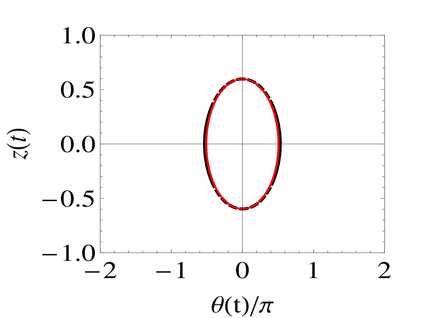
Figure 3: Phase diagrams of the fractional imbalance $z(t)$ vs. macroscopic phase $\theta(t)$ for single component atomic Josephson junctions. The parameters of the double-well potential (2) are the same as in Fig. 2. In both the panels we have set $N=200$ and $K=4.955\times 10^{-3}$.
Left panel: the dashed line represents data from the ODE (19) with $U=0.05\,K$ and $K_{c}=V=0$; the continuous line represents data from the ODE (19) with $U=0.05\,K$, $K_{c}=-1.842\times 10^{-6}$ and $V=2.268\times 10^{-7}$.
The right panel shows the phase diagram for the self-trapping. In this panel the dashed line represents data from the ODE (19) with $U=0.2\,K$ and $K_{c}=V=0$; the continuous line represents data from the ODE (19) with $U=0.2\,K$, $K_{c}=-7.368\times 10^{-6}$ and $V=9.070\times 10^{-7}$. Initial conditions are the same as in Fig. 2. Time is measured in units of $\omega^{-1}$ and energies are measured in units of $\hbar\omega$.

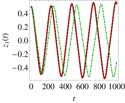
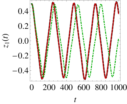
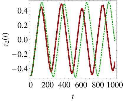
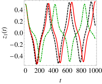
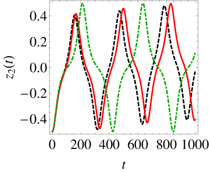
Figure 4: Fractional imbalance $z_{i}(t)$ of the two bosonic species vs. time. The parameters of the double-well potential (2) are chosen to be $b=1$ and $z_{0}=3$. Here, the dashed line represents data from the integration of GPEs (36), the continuous line represents data from the integration of ODEs (3.2), and the dot-dashed line represents data from the integration ODEs (3.2) with $K_{c,i}=V_{i}=K_{c,12}=V_{12}=0$ (i.e. the ODEs analyzed in Ref. [17]). We have fixed $N_{1}=200$ and $N_{2}=100$. Moreover, $K_{1}=K_{2}\equiv K=4.955\times 10^{-3}$, $U_{1}=U_{2}\equiv U=0.1\,K$, $K_{c,1}=K_{c,2}\equiv K_{c}=-3.684\times 10^{-6}$, $V_{1}=V_{2}\equiv V=2.268\times 10^{-7}$. We used the initial conditions $z_{1}(0)=0.5=-z_{2}(0)$ and $\theta_{1}(0)=\theta_{2}(0)=0$. In the top panels we set $U_{12}=-U/20$, $K_{c,12}=-K_{c}/20$, $V_{12}=-V/40$, in the middle panels $U_{12}=-U/2$, $K_{c,12}=-K_{c}/2$, $V_{12}=-V/4$, and in the bottom panels $U_{12}=-U$, $K_{c,12}=-K_{c}$, $V_{12}=-V/2$. Time is measured in units of $(\omega_{1})^{-1}=(\omega_{2})^{-1}\equiv\omega^{-1}$ and energies are measured in units of $\hbar\omega$.

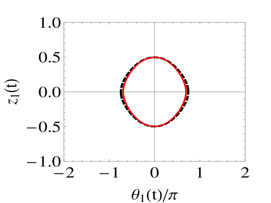
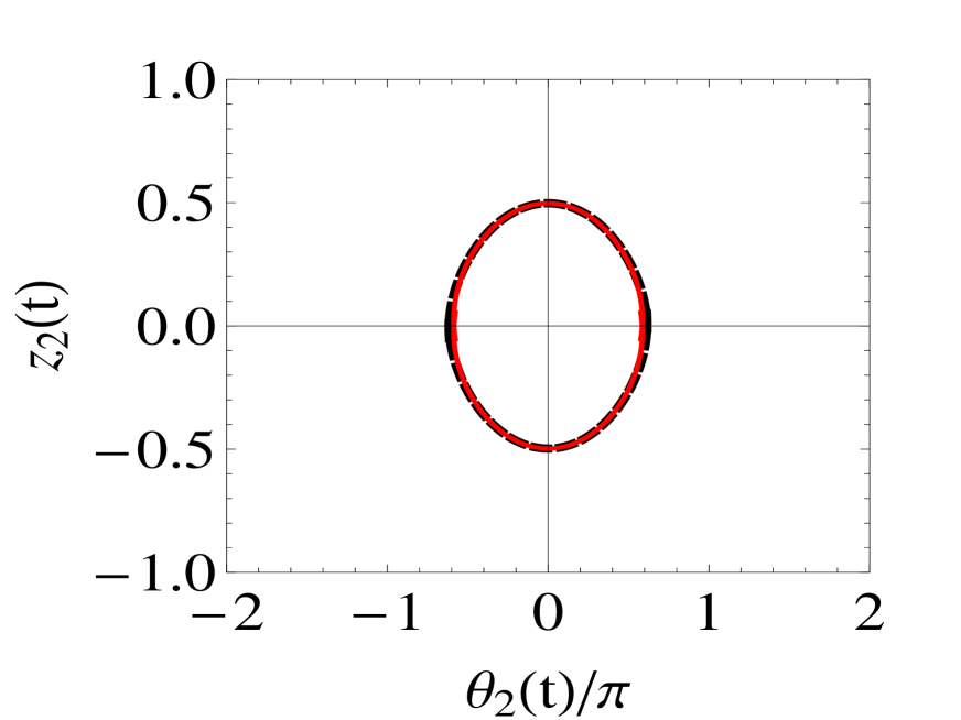
Figure 5: Phase diagrams of the fractional imbalance $z_{i}(t)$ vs. macroscopic phase $\theta_{i}(t)$ of the two bosonic species. The parameters of the double-well potential (2) are the same as in Fig. 4. In both the panels we have set $N_{1}=200$, $N_{2}=100$, $K_{1}=K_{2}\equiv K=4.955\times 10^{-3}$, $U_{1}=U_{2}\equiv U=0.1K$. In both the panels, the dashed line represents data from the ODEs (3.2) with $U_{12}=-U/2$ and $K_{c,i}=V_{i}=K_{c,12}=V_{12}=0$, the continuous line represents data from the ODEs with $U_{12}=-U/2$, $K_{c,1}=K_{c,2}\equiv K_{c}=-3.684\times 10^{-6}$, $V_{1}=V_{2}\equiv V=2.268\times 10^{-7}$, $K_{c,12}=-K_{c}/2$, $V_{12}=-V/4$. Initial conditions are the same as in Fig. 4. Time is measured in units of $(\omega_{1})^{-1}=(\omega_{2})^{-1}\equiv\omega^{-1}$ and energies are measured in units of $\hbar\omega$.

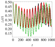
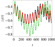
Figure 6: Fractional imbalance $z_{i}(t)$ of the two bosonic species vs. time. In the double-well potential (2) we set $b=1$ and $z_{0}=3$. In this figure the dashed line represents data from the integration of GPEs (36), the continuous line represents data from the integration of ODEs (3.2), and the dot-dashed line represents data from the integration ODEs (3.2) with $K_{c,i}=V_{i}=K_{c,12}=V_{12}=0$ (i.e. the ODEs analyzed in Ref. [17]). We have fixed $N_{1}=200$ and $N_{2}=100$. Moreover, $K_{1}=K_{2}\equiv K=4.955\times 10^{-3}$, $U_{1}=U_{2}\equiv U=0.1\,K$, $K_{c,1}=K_{c,2}\equiv K_{c}=-3.684\times 10^{-6}$, $V_{1}=V_{2}\equiv V=2.268\times 10^{-7}$, $U_{12}=-2\,U$, $K_{c,12}=-2\,K_{c}$ $V_{12}=-V$. Initial conditions are the same as in Fig. 4. Time is measured in units of $(\omega_{1})^{-1}=(\omega_{2})^{-1}\equiv\omega^{-1}$ and energies are measured in units of $\hbar\omega$.

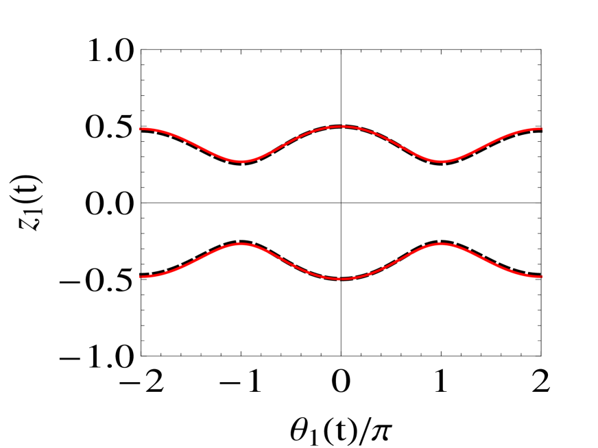
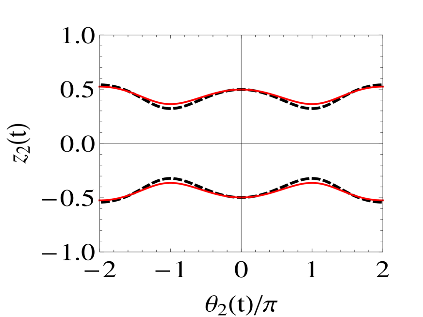
Figure 7: Phase diagrams of the fractional imbalance $z_{i}(t)$ vs. macroscopic phase $\theta_{i}(t)$ of the two bosonic species for the self-trapping. The parameters of the double-well potential (2) are the same as in Fig. 4. In both the panels we have set $N_{1}=200$, $N_{2}=100$, $K_{1}=K_{2}\equiv K=4.955\times 10^{-3}$, $U_{1}=U_{2}\equiv U=0.1\,K$. In both the panels, the dashed line represents data from the ODEs (3.2) with $U_{12}=-2\,U$ and $K_{c,i}=V_{i}=K_{c,12}=V_{12}=0$, the continuous line represents data from the ODEs with $U_{12}=-2\,U$, $K_{c,1}=K_{c,2}\equiv K_{c}=-3.684\times 10^{-6}$, $V_{1}=V_{2}\equiv V=2.268\times 10^{-7}$, $K_{c,12}=-2K_{c}$, $V_{12}=-V$. Initial conditions are the same as in Fig. 4. Time is measured in units of $(\omega_{1})^{-1}=(\omega_{2})^{-1}\equiv\omega^{-1}$ and energies are measured in units of $\hbar\omega$.

We are interested to study the dynamical oscillations of the populations of each condensate between the left and right wells when the the barrier is large enough so that the link is weak. To exploit the strong harmonic confinement in the ($x$-$y$) plane and get the effective one-dimensional (1D) equations describing the dynamics in the $z$ directions, we write the Lagrangian associated to the GPE equations in (31)

$$L = \int d^{3}{\bf r}\,\bigg{(}\bigg{[}\sum_{i=1,2}\bar{\Psi}_{i}\big{(}i\hbar\frac{\partial}{\partial t}+\frac{\hbar^{2}}{2m_{i}}\nabla^{2}\big{)}\Psi_{i}$$

$$- V_{trap}({\bf r})|\Psi_{i}|^{2}-\frac{g_{i}}{2}|\Psi_{i}|^{4}\bigg{]}-g_{ij}|\Psi_{i}|^{2}|\Psi_{j}|^{2}\bigg{)}\;,$$

where $\bar{\Psi}_{i}$ denotes the complex conjugate of $\Psi_{i}$, and $i\neq j$; then, by following the decomposition (8) and the Gaussian approximation for the radial part of wave function, we adopt the ansatz

$$\Psi_{i}(x,y,z,t)=\frac{1}{\sqrt{\pi}a_{\bot,i}}\exp\bigg{[}-\frac{x^{2}+y^{2}}{2a_{\bot,i}^{2}}\bigg{]}f_{i}(z,t)\;,$$ (34)

where the field $f_{i}(z,t)$ obey to $\int_{-\infty}^{+\infty}dz|f_{i}(z)|^{2}=N_{i}$, so that the normalization condition given by Eq. (32) is satisfied. Note that the Gaussian ansatz with the transverse width simply given by $a_{\bot,i}$ is reliable under very strong transverse confinements, namely when $\tilde{g}_{i}|f_{i}|^{2}\ll 2\,\hbar\omega_{i}$ [32]. By inserting the ansatz (34) in Eq. (4) and performing the integration in the radial plane, we obtain the effective 1D Lagrangian for the field $f_{i}(z,t)$. Such an effective 1D Lagrangian reads

$$\tilde{L} = \int dz\,\bigg{(}\bigg{[}\sum_{i=1,2}\bar{f}_{i}\big{(}i\hbar\frac{\partial}{\partial t}+\frac{\hbar^{2}}{2m_{i}}\frac{\partial^{2}}{\partial z^{2}}\big{)}f_{i}$$

$$- (\epsilon_{i}+V_{DW}(z))|f_{i}|^{2}-\frac{\tilde{g}_{i}}{2}|f_{i}|^{4}\bigg{]}-\tilde{g}_{ij}|f_{i}|^{2}|f_{j}|^{2}\bigg{)}\;,$$

where $\epsilon_{i}$ is given by $\displaystyle{\epsilon_{i}=\frac{\hbar^{2}}{2m_{i}a_{\bot,i}^{2}}+\frac{m_{i}\omega_{i}^{2}a_{\bot,i}^{2}}{2}}$. By varying $\tilde{L}$ with respect to $\bar{f}_{i}$, we obtain the 1D GPE for the field $f_{i}$

$$i\hbar\frac{\partial f_{i}}{\partial t}=-\frac{\hbar^{2}}{2m_{i}}\frac{\partial^{2}f_{i}}{\partial z^{2}}+[\epsilon_{i}+V_{DW}(z)+\tilde{g}_{i}|f_{i}|^{2}+\tilde{g}_{ij}|f_{j}|^{2}]f_{i}\;.$$ (36)

In the presence of a single bosonic component, $g_{12}=0$; then, the two coupled 1D GPEs Eq. (36), omitting the species index $i$, reduce to

$$i\hbar\frac{\partial f}{\partial t}=-\frac{\hbar^{2}}{2m}\frac{\partial^{2}f}{\partial z^{2}}+[\epsilon+V_{DW}(z)+\tilde{g}|f|^{2}]f\;.$$ (37)

Now, we observe that it is possible to write the fields $f_{i}$, ($i=1,2$), by using the two-mode approximation as done, for example, in Ref. [17]

$$f_{i}(z,t)=\psi_{L,i}(t)\phi_{L,i}(z)+\psi_{R,i}(t)\phi_{R,i}(z)$$

$$\psi_{\alpha,i}(t)=\sqrt{N_{\alpha,i}(t)}\exp(i\theta_{\alpha,i}(t))\;,$$ (38)

with $\phi_{\alpha,i}(z)$ constructed as discussed in Sec. III, see Eq. (3). Then, one takes into account the overlaps both between $\phi_{\alpha}$’s localized in the same well and between $\phi_{\alpha}$’s localized in different wells. By following the same path as in Ref. [17], when the inter-species coupling constant $g_{12}$ is finite, it is possible to recover Eqs. (3.2) for binary AJJs, while for $g_{12}$ equal to zero one gets back the Eqs. (19) for single component AJJs .

At this point - both for single component and for two components AJJs - we may compare the predictions of the ODEs, Eqs. (19) and (3.2), and those of the GPEs, Eqs. (37) and (36). The results of this analysis are reported in Fig. 2 for the single component case, and in Figs. 4, 6 for the two components case. In obtaining Fig. 2 we have fixed the parameters $b$ and $z_{0}$ of the double-well potential (2). Then, by using the functions (3) into the third of Eqs. (3.1), we have obtained the tunneling amplitude $K$. We have keeped fixed $K$ and we have plotted the predictions of the ODEs (19) for $z(t)$ in correspondence to different intra-species interactions both when $K_{c}$ and $V$ are zero - dot-dashed lines - and in the presence of $K_{c}$ and $V$ - continuous lines; the dashed lines represent $z(t)$ obtained by numerically integrating the GPE (37). In Figs. 4, 6 we have fixed the tunneling amplitude $K_{i}$ - as done previously in the single component case - and the intra-species interaction $U_{i}$, and we have plotted the predictions of the ODEs (3.2) for $z_{i}(t)$ in correspondence to different inter-species interactions both when $K_{c,i}$, $V_{i}$, $K_{c,12}$, $V_{12}$ are all equal to zero - dot-dashed lines - and in the presence of $K_{c,i}$, $V_{i}$, $K_{c,12}$, $V_{12}$ - continuous lines; again, the dashed lines represent $z_{i}(t)$ obtained by numerically integrating the GPEs (36). In the two top panels of Fig. 2 and in all the panels of Fig. 4, we have plotted the temporal evolution of the bosonic fractional imbalances $z$ when they oscillate around a zero time-averaged value, i.e. $\langle z(t)\rangle=0$. We see that the usually-neglected nonlinear terms play a crucial role in order to improve the agreement between the GPEs the ODEs predictions. In fact, neglecting these terms, the solutions of ODEs and GPEs diverge rather rapidly, as shown by dot-dashed lines in Fig. 2 - single component AJJs - and by dot-dashed lines in Fig. 4, for two components AJJs. The two bottom panels of Fig. 2 show the results of our analysis when the intra-species interaction amplitude $U$ is sufficiently large to induce oscillations of $z(t)$ around a non zero time-averaged value, that is the self-trapping. We see that the inclusion within the description of the system of the usually-neglected nonlinear terms produces an improvement in the agreement between the ODEs and GPE predictions. In the two components case, from Fig. 4 we can see that the nonlinearity associated to the intra-species interaction is not strong enough to induce oscillations of $z_{i}$ around a non zero time-averaged value. Nevertheless, if the inter-species interaction is sufficiently large, oscillations of $z_{i}$ around $\langle z_{i}(t)\rangle\neq 0$ are observed. We have reported this kind of behavior for both the components in Fig. 6. From this figure we can see that, especially in the case of large inter-species interaction, the role played by the parameters describing the overlaps between $\phi_{\alpha}$’s localized in different wells becomes essential to improve the agreement between the ODEs and the GPEs predictions. Moreover, in Fig. 3 - single component AJJs - and in Fig. 5 and Fig. 7 - two components AJJs - we show the phase-plain portraits of the dynamical variables $z_{i}$ and $\theta_{i}$ for different values of the macroscopic parameters (3.1) and (3.2) (see Figs. 3, 5, 7 for the details). These figures show the comparison between the trajectories in the phases space obtained by integrating the ODEs in the absence of the usually-neglected nonlinear terms (dashed lines), and the trajectories obtained from the improved version of ODEs (continuous lines). In particular, the left and the right panels of Fig. 3 show the phases space trajectories for the Josephson and self-trapping regimes, respectively, for single component AJJs. For two components AJJs, in Fig. 5 we have plotted the phases space trajectories for the Josephson regime, and in Fig. 7 we have plotted the phases space trajectories when the system is self-trapped. From Figs. 3, 5, 7 we can see that the trajectories predicted when the ODEs Eqs. (19) and (3.2) are solved in the absence of the usually-neglected nonlinear terms are sufficiently close to those predicted when these ODEs are solved in the presence of the aforementioned terms. Then, the dynamical evolution predicted by the standard ODEs reveals to have a good degree of reliability.

5 Conclusions

We have analyzed atomic Josephson junctions for a single Bose gas and for binary mixtures of bosons in a double-well potential along the axial direction and a strong harmonic confinement in the transverse directions. We have shown that for both the cases the Hamiltonian belongs to the extended Bose-Hubbard model and besides the density-density interaction it contains the pair hopping and collisionally induced hopping terms. These terms derive from the overlaps between wave functions localized in different potential wells. We started from these Hamiltonian models and established connections with spin Hamiltonians. Proceeding from these, we have discussed the possibility to discriminate, under certain conditions, different dynamical regimes sustained by the bosonic junctions. From the mean field analysis of the equations of motion for the single-particle operators involved in the extended Bose-Hubbard Hamiltonians, we have obtained the ordinary differential equations that control the macroscopic dynamics of the atomic Josephson junctions. Within the analysis of the atomic Josephson junctions macroscopic dynamics we have plotted the phase-plane portraits of the dynamical variables (fractional imbalance-relative phase) showing that the inclusion of the aforementioned collisionally induced hopping and pair hopping terms are crucial to get good agreement between the dynamics of the Josephson model described by ordinary differential equations and the one of the time dependent Gross-Pitaevskii equations, especially when the atom-atom interaction is strong.

Finally, it is important to remark that the obtained results are of general validity also for more confining (e.g. not saturating to zero at large distances) double-well potentials. Nevertheless, it is possible to design a model of pair hopping and collisionally induced hopping for bosonic atoms that is physically meaningful when optical lattices play the role of confining potentials. Physical effects related to pair hopping and collisionally induced hopping should be observable in generalizations of current experiments to detect the superfluid and insulating phases [33].

This work has been partially supported by Fondazione CARIPARO through the Project 2006: ”Guided solitons in matter waves and optical waves with normal and anomalous dispersion”. G. M. thanks A. B. Kuklov and B. V. Svistunov for useful comments.

References

References

• [1] S. N. Bose, Z. Phys. 26, 178 (1924); A.Einstein, Sitzungsber. K. Preuss. Akad. Wiss., Phys. Math. K1. 22, 261 (1924).
• [2] M. H. Anderson, M. R. Matthews, C. E. Wieman, and. E. A. Cornell, Science 269, 198 (1995); K. B. Davis, M. O. Mewes, M. R. Andrews, N. J. van Druten, D. S. Durfee, D. M. Kurn, and W. Ketterle, Phys. Rev. Lett. 75, 3969 (1995); C. C. Bradley, C. A. Sackett, J. J. Tollett, and R. G. Hulet, ibid. 75, 1687 (1995).
• [3] A. J. Leggett and F. Sols, Found. Phys. 21, 353 (1991); I. Zapata, F. Sols, and A. J. Leggett, Phys. Rev. A 57, R28 (1998).
• [4] A. J. Leggett, Rev. Mod. Phys. 73, 307 (2001).
• [5] A. Smerzi, S. Fantoni, S. Giovanazzi, and S. R. Shenoy, Phys. Rev. Lett. 79, 4950 (1997); S. Raghavan, A. Smerzi, S.Fantoni, and S. R. Shenoy, Phys. Rev. A 59, 620 (1999).
• [6] L. Salasnich, A. Parola, L. Reatto, J. Phys. B: At. Mol. Opt. Phys. 35, 3205-3216 (2002).
• [7] M. Salerno, Laser Phys. 4, 620-625 (2005).
• [8] A. Barone and G. Paternò, Physics and Applications of the Josephson effect (Wiley, New York, 1982); H. Otha, in SQUID: Superconducting Quantum Devices and their Applications, edited by H.D. Hahlbohm and H. Lubbig (de Gruyter, Berlin, 1977).
• [9] M. Albiez, R. Gati, J. Fölling, S. Hunsmann, M. Cristiani, M. K. Oberthaler, Phys. Rev. Lett. 95, 010402 (2005).
• [10] R. Gati and M. K. Oberthaler, J. Phys. B: At. Mol. Opt. Phys. 40, R61-R89 (2007).
• [11] C. J. Milburn, J. Corney, E. M. Wright, and D. F. Walls, Phys. Rev. A 55, 4318 (1997).
• [12] G. Thalhammer, G. Barontini, L. De Sarlo, J. Catani, F. Minardi, and M. Inguscio, Phys. Rev. Lett. 100, 210402 (2008).
• [13] S. B. Papp and C. E. Wieman, Phys. Rev. Lett. 97, 180404 (2006).
• [14] X. Xu, L. Lu, Y. Li, Phys. Rev. A 78, 043609 (2008).
• [15] I. I. Satija, P. Naudus, R. Balakrishnan, J. Heward, M. Edwards, C.W. Clark, Phys. Rev. A 79, 033616 (2009).
• [16] B. Julia-Diaz, M. Guilleumas, M. Lewenstein, A. Polls, A. Sanpera, Phys. Rev. A 78, 023616 (2009).
• [17] G. Mazzarella, M. Moratti, L. Salasnich, M. Salerno and F. Toigo, J. Phys. B: At. Mol. Opt. Phys. 42, 125301 (2009).
• [18] B. Julia-Diaz, M. Mele-Messeguer, M. Guilleumas, and A. Polls, Phys. Rev. A 80, 043622 (2009).
• [19] C. Wang, P. G. Kevrekidis, N. Whitaker and B. A. Malomed, Physica D 327, 2922-2932 (2008).
• [20] G.Mazzarella, S. M. Giampaolo, F. Illuminati, Phys. Rev. A 76, 013625 (2006).
• [21] L. Amico, G.Mazzarella, S. Pasini, F. S. Cataliotti, New J. Phys, 12, 013002 (2010).
• [22] A. B. Kuklov and B. V. Svistunov, Phys. Rev. Lett. 90, 100401 (2003).
• [23] P. Buonsante, S. M. Giampaolo, F. Illuminati, V. Penna, A. Vezzani, Phys. Rev. Lett. 100, 240402 (2008); P. Buonsante, S. M. Giampaolo, F. Illuminati, V. Penna, A. Vezzani, Eur. Phys. J. B 68, 427 (2009).
• [24] T. Keilmann, J. I. Cirac, T. Roscilde, Phys. Rev. Lett. 102, 255304 (2009).
• [25] G. Ferrini, A. Minguzzi, F. W. Hekking, Phys. Rev. A 78, 023606(R) (2008).
• [26] D. V. Averin, T. Bergeman, P. R. Hosur, and C. Bruder, Phys. Rev. A 78, 031601(R) (2008).
• [27] D. Ananikian and T. Bergeman, Phys. Rev. A, 73, 013604 (2006).
• [28] L. Landau and L. Lifshitz, Course in Theoretical Physics, Vol. 3, Quantum Mechanics: Non-Relativistic Theory, (Pergamon, New York, 1959).
• [29] This definition of $\hat{J}_{x}$ and $\hat{J}_{z}$ follows that of Refs. [4, 27]. A definition with exchanged $\hat{J}_{x}$ and $\hat{J}_{z}$ is also widely used in literature - see e.g. [25] - and in theoretical quantum optics textbooks - see e.g. [30].
• [30] S. M. Barnett and P. M. Radmore, Methods in Theoretical Quantum Optics, (Oxford University Press, New York, 1997).
• [31] A. B. Kuklov and B. V. Svistunov, e-mail communications.
• [32] L. Salasnich, A. Parola, and L. Reatto, Phys. Rev. A 65, 043614 (2002); L. Salasnich, A. Parola, and L. Reatto, Phys. Rev. A 70, 013606 (2004); L. Salasnich and B. A. Malomed, Phys. Rev. A 74, 053610 (2006).
• [33] M. Eckholt and J. J. García Ripoll, Phys. Rev. A 77, 063603 (2008).