Turbulent small-scale dynamo action in solar surface simulations

Abstract

We demonstrate that a magneto-convection simulation incorporating essential physical processes governing solar surface convection exhibits turbulent small-scale dynamo action. By presenting a derivation of the energy balance equation and transfer functions for compressible magnetohydrodynamics (MHD), we quantify the source of magnetic energy on a scale-by-scale basis. We rule out the two alternative mechanisms for the generation of small-scale magnetic field in the simulations: the tangling of magnetic field lines associated with the turbulent cascade and Alfvénization of small-scale velocity fluctuations (“turbulent induction”). Instead, we find the dominant source of small-scale magnetic energy is stretching by inertial-range fluid motions of small-scale magnetic field lines against the magnetic tension force to produce (against Ohmic dissipation) more small-scale magnetic field. The scales involved become smaller with increasing Reynolds number, which identifies the dynamo as a small-scale turbulent dynamo.

1 Introduction

Generically, three-dimensional (3D) magnetohydrodynamic turbulence excites dynamo action when the magnetic Reynolds number exceeds a critical threshold (such that amplification by stretching dominates over Ohmic dissipation). That turbulence could amplify magnetic energy by the random stretching of field lines was proposed by Batchelor (1950) and first demonstrated in direct numerical simulations by Meneguzzi et al. (1981). Many turbulent flows with high enough Reynolds numbers support dynamo action. Solar surface convection is likely such a flow, but the relation to the global solar dynamo is not clear (Ossendrijver, 2003). There is evidence for local dynamo action near the solar surface (Petrovay & Szakaly, 1993), and the question of whether surface convection can support a turbulent dynamo is the focus of the present work.

The simulations of Meneguzzi et al. (1981) demonstrated turbulent dynamos with dramatically different characteristics. In one case, magnetic energy grows at scales smaller than the forcing scale of fluid motions. This defines small-scale dynamo (SSD) or fluctuation dynamo action (see, e.g., Iskakov et al. 2007). In the other case, magnetic energy grows at scales larger than the forcing scale: large-scale dynamo. Such large-scale dynamos are often studied in the framework of mean-field theory (see, e.g., Krause & Raedler 1980; Covas et al. 1997; Field et al. 1999; Field & Blackman 2002) which suggests that the production of large-scale magnetic energy is related to the lack of reflectional symmetry in the small-scale velocity fluctuations (e.g., from helical motions). A more intuitive picture is that kinetic helicity creates magnetic helicity through Alfvénization, which then goes through an inverse cascade to large scales (Pouquet et al., 1976) – the magnetic tension force expands coils in the magnetic field lines. Symmetry breaking (e.g., helicity) is not required for small-scales dynamos and it is widely believed that sufficiently chaotic 3D flows will be SSDs. Near the solar surface, the convective (granulation) time scale is much shorter than the rotation period, so that a flow with negligible net helicity results and large-scale dynamo action is not expected. However, surface convection is expected to be sufficiently chaotic to be a small-scale dynamo.

The origin and properties of the quiet-Sun intra-network magnetic field provide observational evidence of and arguments for local small-scale dynamo action on the Sun. Firstly, from a flux-transport model, Petrovay & Szakaly (1993) conclude that the decay of active regions (or of flux tubes not quite rising to the surface) is insufficient to account for the observed intra-network magnetic fields. A source term is required in their model to match the observations and they conclude that the physical interpretation of this term is small-scale dynamo action in the convection zone. Secondly, small-scale dynamo action is also consistent with high resolution magnetograms of the intra-network. These show mixed polarity fields on small scales (variously called the magnetic carpet or the salt-and-pepper pattern; Title & Schrijver 1998; Hagenaar et al. 2003). The fractal nature of these opposite polarities extends down to the resolution limit of the observations (Pietarila Graham et al., 2009). Furthermore, the amount of observed small-scale flux is not dependent on the solar cycle, nor does it show any latitudinal dependence (Hagenaar et al., 2003; Sánchez Almeida, 2003; Trujillo Bueno et al., 2004). These results all suggest that the source of quiet-Sun magnetic field is independent of the global dynamo. Lastly, turbulent convection has been shown to drive dynamo action in numerical simulations of Boussinesq convection without rotation (Cattaneo, 1999; Cattaneo et al., 2003). Observations and simulations together provide evidence, then, of a small-scale dynamo driven by turbulence at the solar surface.

An alternative interpretation of the observations is that the small-scale field results from turbulence acting on the large-scale magnetic field from the global dynamo. Such induced small-scale fields could result from two different processes. One process is the turbulent tangling, sometimes called “shredding,” of field lines which moves magnetic energy to smaller scales as part of the turbulent energy cascade. However, the turbulent cascade is associated with power-law energy spectra and, therefore, the amount of small-scale intra-network flux should change as the strength of any large-scale background field changes over the solar cycle. This contradicts observations (Hagenaar et al., 2003; Sánchez Almeida, 2003; Trujillo Bueno et al., 2004). A similar argument, against the decay of active regions as the source of intra-network flux, has been put forward by Sánchez Almeida et al. (2003). Additionally, the total unsigned magnetic flux (and energy) in active regions even during solar maximum is less than the unsigned magnetic flux (and energy) contained in the quiet-Sun (Sánchez Almeida, 2004; Trujillo Bueno et al., 2004), making decay from active regions as a source of the small-scale field very unlikely.

The second process for producing small-scale magnetic field from large-scale field, called turbulent induction (Schekochihin et al., 2007), involves the stretching of a uniform (or large scale) background magnetic field by turbulent fluid motions which excites Alfvénic magnetic fluctuations on the same scale as the turbulent fluid eddies. Alfvénic turbulent induction will be present whenever there is a significant background field. In the presence of both a flow capable of sustaining small-scale dynamo action and a large-scale magnetic field, the small-scale dynamo and Alfvénic induction may compete as the source of small-scale field.

Given the prevalence of turbulent dynamos in homogeneous, isotropic turbulence, such dynamo action is expected in the Sun unless additional physics can be identified which would suppress it. Two points are often raised to argue that a small-scale dynamo cannot operate in the Sun. Firstly, turbulent eddies smaller than the characteristic scale of the magnetic field act like a turbulent magnetic diffusivity and could inhibit dynamo action. This is an important concern for the Sun (and other stars) because the kinetic Reynolds number, $Re\equiv v_{0}l_{0}/\nu$ ($v_{0}$ and $l_{0}$ being typical velocity and length scales, and $\nu$ the kinematic viscosity), is much larger than the magnetic Reynolds number, $Re_{M}\equiv v_{0}l_{0}/\eta$ ($\eta$ being the magnetic diffusivity). Their ratio, the magnetic Prandtl number, $P_{M}\equiv Re_{M}/Re$, is approximately $10^{-5}$ near the solar surface. The critical magnetic Reynolds number for turbulent dynamo action, $Re_{M}^{C}$, sharply increases with decreasing $P_{M}$ and it has been suggested that $Re_{M}^{C}$ goes to infinity as $P_{M}$ goes to zero (Rogachevskii & Kleeorin, 1997; Boldyrev & Cattaneo, 2004; Schekochihin et al., 2005). However, recent numerical simulations attest that $Re_{M}^{C}$ approaches a plateau for $P_{M}\ll 1$ both with physical (Laplacian) viscosity (Ponty et al., 2005) and with hyperviscosity (Iskakov et al., 2007). Baring the identification of a new length scale in the problem, these results indicate that, for magnetohydrodynamics (MHD), small-scale dynamo action remains possible in the asymptotic limit as $P_{M}$ goes to zero. Additionally, a laboratory dynamo with liquid sodium ($P_{M}\approx 10^{-5}$) resulting from unconstrained turbulence has been demonstrated (Monchaux et al., 2007). This establishes that a turbulent (at least, a large-scale) dynamo is possible at values of $P_{M}$ corresponding to the solar plasma (Monchaux et al., 2009).

The second suppression argument is that, unlike the Cattaneo (1999) Boussinesq simulation, the Sun is strongly stratified and magnetic flux is swept into the downflows and subject to long recirculation times (Stein et al., 2003). In their stratified simulations with open boundaries, Stein et al. (2003) found no evidence of dynamo action for surface convection. Their magnetic Reynolds number, however, was below the critical value. Vögler & Schüssler (2007) have demonstrated that surface convection with little field recirculation and strong density stratification (as well as other physical effects present in the Sun) can support local dynamo action when $Re_{M}\gtrsim 2000$. We will determine if this local dynamo action is a small-scale turbulent dynamo. Currently, no other likely suppression mechanisms for small-scale dynamo action in the intra-network photosphere are known.

The magnetic energy spectrum of the Vögler & Schüssler (2007) dynamo peaks at scales smaller than the energy-containing scale of the fluid motions, which is suggestive of a small-scale dynamo. However, except in the most idealized of simulations, non-zero time-averaged mean flows exist for times ($\sim 10\,$minutes for photospheric convection) long compared to inertial-range eddy-turnover times (e.g., $\sim 6\,$seconds at a scale of $1\,$km). Therefore, even in the absence of net helicity, this mean flow can act as a low $Re_{M}$ dynamo that produces magnetic field near the mean-flow scale (Ponty et al., 2007), $\approx 1\,$Mm for convective granulation. This would not be a small-scale dynamo; it would still have small-scale magnetic field produced from either the turbulent cascade or from Alfvénic turbulent induction. In order to fully understand what is occurring, it is important to disentangle the possible sources of small-scale magnetic energy and properly identify the dynamo mechanism (Schekochihin et al., 2007).

We have employed transfer analysis to measure, scale by scale, the relative strengths of the sources of magnetic energy: turbulent cascade, Alfvénic turbulent induction, and dynamo action (by stretching of field lines) in the simulations of Vögler & Schüssler (2007). The scales involved in the dynamo and their dependence on Reynolds number as well as growth rates and energy spectra allow us to determine that the dynamo is a turbulent small-scale dynamo.

2 Data and methods

We use MURaM (Vögler, 2003; Vögler et al., 2005) to perform simulations for a rectangular domain of horizontal extent $4.86\times 4.86\,$Mm² and a depth of $1.4\,$Mm ($800\,$km below and $600\,$km above the simulated solar surface). The sides boundaries are periodic in both horizontal directions. The open lower boundary assumes upflows to be vertical, $v_{x}=v_{y}=\partial_{z}v_{z}=0$; for downflows vertical gradients are set to zero, $\partial_{z}v_{x}=\partial_{z}v_{y}=\partial_{z}v_{z}=0$. The upper boundary is closed. The magnetic field is vertical at upper and lower boundaries: $B_{x}=B_{y}=\partial_{z}B_{z}=0$. This ensures that there is no Poynting flux into or out of the box. The magnetic diffusivity is increased in the lower $150\,$km of the box in order to well resolve the diffusive boundary layer (Vögler & Schüssler, 2007). These boundary conditions allow the convective downflows to leave the box and, thus, simulate an artificially isolated surface layer. These same downflows drag magnetic field to the lower region of enhanced diffusivity where it can be eliminated (this simulates the fact that the field should not be available for further stretching due to long recirculation times; see Stein et al. 2003). The upper $600\,$km of the box is convectively stable and the lower $800\,$km of the box is convectively unstable. The convection is driven by radiative cooling (calculated using grey radiative transfer and the Rosseland mean opacities) at the surface where the optical depth is unity. The effects of partial ionization are included in the equation of state. These simulations are then so-called “realistic” simulations of a portion of the solar surface layer including compressibility and stratification (4 orders-of-magnitude variation in the density), radiative energy transport, partial ionization, and little recirculation. “Realistic” is used here to distinguish them from a class of “idealistic” simulations of incompressible, isotropic, homogeneous, and triply-periodic MHD turbulence. Of course, neither type of simulation is able to achieve the Reynolds and Prandtl numbers of the Sun, but aside from this, MURaM simulations include more of the physics relevant to the near-surface layers of the Sun. Our aim is to determine if these effects inhibit turbulent small-scale dynamo action or overshadow it with some other mechanism.

Table 1: Properties of MURaM dynamo runs: grid resolution, effective magnetic Prandtl number, $P_{M,{\rm eff}}$, magnetic diffusivity, $\eta$, magnetic Reynolds number, $Re_{M}$ based on $v_{rms}\approx 3.3\,$km/s and a length scale of $1\,$Mm, and kinematic dynamo regime $e-$folding time, $\gamma^{-1}$.

Simulation	Grid Resolution (km)	$P_{M,{\rm eff}}$	$\eta$ (cm2 s-1)	$Re_{M}$	$\gamma^{-1}$ (s)
Run 1	$9\times 9\times 10$	$\sim 2.0$	$1.6\cdot 10^{10}$	$\approx 2100$	$1600$
Run 2	$7.5\times 7.5\times 10$	$\sim 1.3$	$1.25\cdot 10^{10}$	$\approx 2600$	$660$
Run 3-P	$5\times 5\times 7$	$\sim 0.8$	$1.25\cdot 10^{10}$	$\approx 2600$	$1200$
Run 3	$5\times 5\times 7$	$\sim 1.1$	$6.25\cdot 10^{9}$	$\approx 5300$	$230$
Run 4	$4\times 4\times 4$	$\sim 1.1$	$4\cdot 10^{9}$	$\approx 8300$	$150$

Dynamo runs with increasing resolution and Reynolds numbers have been carried out. Table 1 summarizes the parameters of the runs. Figure 1 displays the time evolution of magnetic energies. Run 2 has previously been reported (as “Run C”) for dynamo action in Vögler & Schüssler (2007). All runs start from an initial hydrodynamic case plus weak magnetic seed field. There is an initial growth of $E_{M}$ for about $3\,$minutes due to flux expulsion and convective intensification followed by the linear (kinematic) phase during which magnetic energy grows exponentially with time and the magnetic field is too weak to affect fluid motions. The lower resolution simulations are continued until the nonlinear phase when the back reaction of the Lorentz force on fluid motions becomes important and the magnetic energy begins to saturate.

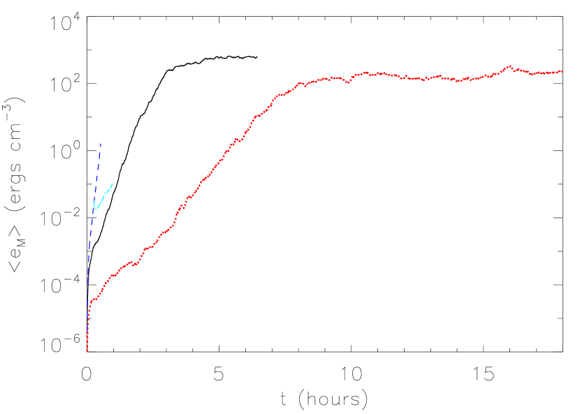
Figure 1: Mean magnetic energy density, $\langle e_{M}\rangle$, versus time, $t$, for dynamo simulations. Shown are Run 1 (red, dotted), Run 2 (black, solid), Run 3 (blue, dashed), and Run 3-P (cyan, dash-dotted).

For all MURaM simulations, constant magnetic diffusivity is employed (outside the region of enhanced diffusivity near the bottom boundary), but artificial shock resolving and hyperviscosity are applied to the momentum equations (see Vögler et al. 2005 for details). This approach allows us to reach high effective kinetic Reynolds number, $Re_{\rm eff}$, without a prohibitively small time step. No value of viscosity is defined, but $Re_{\rm eff}$ can be estimated from the energy spectra (Figure 2). The estimate of the effective Reynolds number is derived from the representative length scales: the velocity Taylor microscale, $\lambda_{V}$,

$$\lambda_{V}^{2}=\langle v^{2}\rangle\big{/}\langle\omega^{2}\rangle=\int_{0}^{\infty}E_{V}(k_{\perp})dk_{\perp}\big{/}\int_{0}^{\infty}k_{\perp}^{2}E_{V}(k_{\perp})dk_{\perp}$$ (1)

where $E_{V}(k_{\perp})$ is the horizontal velocity spectrum and the integral scale for the turbulent motions, $L_{0}$,

$$L_{0}=\int_{0}^{\infty}k_{\perp}^{-1}E_{V}(k_{\perp})dk_{\perp}\big{/}\int_{0}^{\infty}E_{V}(k_{\perp})dk_{\perp}\,.$$ (2)

The effective Reynolds numbers of the simulations is given by (Batchelor, 1953; Weygand et al., 2007),

$$Re_{\rm eff}\propto\bigg{(}\frac{L_{0}}{\lambda_{V}}\bigg{)}^{2}\,,$$ (3)

where the constant of proportionality is unknown. We can also determine the magnetic energy Taylor scale, $\lambda_{M}$,

$$\lambda_{M}^{2}=\int_{0}^{\infty}E_{M}(k_{\perp})dk_{\perp}\big{/}\int_{0}^{\infty}k_{\perp}^{2}E_{M}(k_{\perp})dk_{\perp}\,.$$ (4)

This allows us to estimate the effective magnetic Prandtl number,

$$P_{M,{\rm eff}}\propto\bigg{(}\frac{\lambda_{V}}{\lambda_{M}}\bigg{)}^{2}\,.$$ (5)

We determine the constant of proportionality from an incompressible, isotropic, and homogeneous dynamo simulation. We employed a pseudospectral code (Gómez et al., 2005a, b) and forced the velocity field with a superposition of harmonic modes with random phases, the resolution was $256^{3}$ grid points, and $P_{M}=4$. From this calibration of Eq. (5), we estimated that the magnetic Prandtl numbers in our MURaM runs are between 1 and 2 (see Table 1).

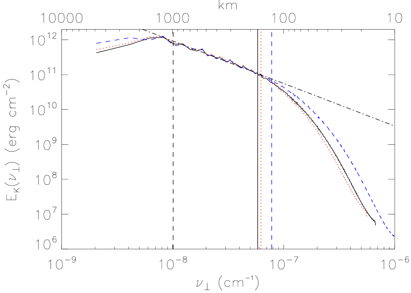
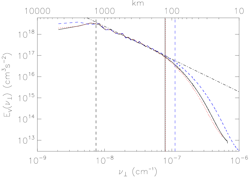
Figure 2: Left: Kinetic energy spectrum, $E_{K}$, versus horizontal spatial frequency, $\nu_{\perp}$, for Run 2 (black, solid) averaged over $t\in[2.2,2.4]\,$hr, for Run 1 (red, dotted) averaged over $t\in[0.2,1.4]\,$hr, and for Run 3 (blue, dashed) averaged over $t\in[0.1,0.5]\,$hr. The vertical lines represent the integral scale ($\approx 10^{8}\,$cm) and Taylor scales near the beginning and end of the inertial range where we identify a power-law scaling: $k_{\perp}^{-1.2}$ (dot-dashed line). Right: Velocity spectrum, $E_{V}$, versus $\nu_{\perp}$ for the same runs. The identified power law extends to smaller scales and has a slope of $-1.54\pm 0.07$.

We find power-law scalings, $k_{\perp}^{\beta}$, in the inertial range with $\beta=-1.2\pm 0.1$ for the kinetic energy spectrum and $\beta=-1.54\pm 0.07$ for the velocity spectrum. Using second-order longitudinal structure functions for the velocity (not shown), we determined that at scales larger than $\approx 50\,$km (approximately half a pressure scale height of the vertical stratification at the surface) the flow is anisotropic. The strong vertical downflows in the convectively unstable lower $800\,$km of the box are the source of this anisotropy. Because of the anisotropy, our spectra cannot be compared to the $\beta=-5/3$ from the Kolmogorov spectrum for homogeneous, isotropic turbulence (see, e.g.,Frisch 1995).

3 Comparison with “idealistic” small-scale dynamos

3.1 Incompressible, isotropic kinematic/linear phase

In the kinematic regime, where the Lorentz force is insignificant, the magnetic energy is observed to grow exponentially, $E_{M}\sim\exp\gamma t$ ($\gamma$ is the growth rate). For turbulent dynamos (with $P_{M}\ll 1$), the growth rate scales as

$$\gamma\sim Re_{M}^{1/2}\,,$$ (6)

though no simulation has yet exceeded $Re_{M}^{C}$ enough to observe the predicted scaling (see, e.g., Schekochihin et al. 2007). For the large magnetic Prandtl case, $P_{M}\geq 1$, we expect $\gamma\sim Re^{1/2}$. Again, this scaling has not yet been found in any simulations (Schekochihin et al., 2004). Other predictions about the kinematic (linear) phase of the small-scale dynamo are due to the exactly solvable Kazantsev model (see Schekochihin et al. 2004 and references therein). This model predicts that the amplitude of each (Fourier) mode grows exponentially at the same rate (see also, Mininni et al. 2005b for a growth rate analysis) and that the magnetic energy spectrum at large scales follows a $k^{3/2}$ scaling.

3.2 MURaM kinematic/linear phase

For the MURaM dynamo, the dependence of growth rate on Reynolds number is shown in Figure 3. The growth rate is an increasing function of Reynolds number. This indicates that the dynamo is a small-scale (inertial range) process. We find that we have not yet sufficiently exceeded $Re_{M}^{C}$ (from Vögler & Schüssler 2007 and Run 1, $1300<Re_{M}^{C}<2100$) to observe the predicted power-law scaling. Instead, at the Reynolds numbers we can achieve, the growth rate depends almost linearly on $Re_{M}$ (dashed line). Higher resolution simulations will be required to determine if there is, indeed, an asymptotic power-law.

Figure 3: Growth rate of magnetic energy, $\gamma$, versus magnetic Reynolds number, $Re_{M}$ for Run 1, Run 2, Run 3, and Run 4. Also shown is a linear fit (dashed) and the theoretical $Re_{M}^{1/2}$ scaling (dotted) for reference.

In Figure 4, we have plotted magnetic energy spectra, $E_{M}(\nu_{\perp})$, at different times from the beginning of the linear regime (including the end of the flux expulsion phase) for Run 3. Power laws can be fit to the magnetic spectrum for scales larger than $\lambda_{K}$, where magnetic energy is growing at the same rate for all scales. A power law is in contrast to the case of a laminar dynamo and indicates that a turbulent, self-similar process underlies the dynamo mechanism. We find $E_{M}(k)\propto k_{\perp}^{\beta}$ with $\beta=0.83\pm 0.04$. The results from Run 2 are $\beta=0.63\pm 0.06$ and for Run 1, $\beta=0.53\pm 0.05$. None of these slopes agree with $k^{3/2}$ from the isotropic Kazantsev case, but are not expected to because of the anisotropy of fluid motions in the downflows. We find, however, that the degree of anisotropy decreases with increasing $Re_{\rm eff}$ for the runs and the exponent $\beta$ becomes closer to $3/2$. This decrease in anisotropy is due to the generation of stronger horizontal fluctuations by the turbulence (strong vertical fluctuations are induced by the convective driving). In summary, we find that the general character of the MURaM dynamo is similar to the incompressible, isotropic, small-scale dynamo but the spectral index differs.

Figure 4: Magnetic energy spectra, $E_{M}(\nu_{\perp})$ (solid lines), for Run 3 for $t=11$, $16$, $23$, $28$, and $31\,$min (kinematic phase). The vertical dashed line is the kinetic Taylor scale. Above this scale, the magnetic energy spectra follow a power law (indicating a turbulent dynamo process) with all scales growing at the same temporal rate. The time-averaged kinetic energy spectrum (dashed line) is compensated by $k_{\perp}^{1.2}$ so the inertial range is flat.

4 Transfer analysis (kinematic phase)

It is clear that the magnetic energy is peaking at scales nearly one order of magnitude smaller than the energy-containing scale of the fluid motions, $L_{0}\approx 1\,$Mm (see Figure 4). This indicates small-scale dynamo action, with one caveat. As discussed in Section 1, “mean flows” might give rise to a Mm-scale dynamo. We must, therefore, disentangle three possible sources of small-scale magnetic energy: the tangling of field lines caused by the turbulent energy cascade, Alfvénic response of larger-scale field to smaller scale velocity fluctuations (Alfvénic turbulent induction), and dynamo stretching of magnetic field lines (Schekochihin et al., 2007). This can be accomplished by spectral transfer analysis.

Spectral transfer analysis was introduced by Kraichnan (1967) and is widely used to understand incompressible turbulent processes in both two (e.g., Maltrud & Vallis 1993; Eyink 2006) and three (e.g., Zhou 1993) dimensions for both Navier-Stokes (e.g., Kraichnan 1971; Mininni et al. 2008) and MHD (e.g., Debliquy et al. 2005; Verma et al. 2005). In Appendix A.1, we extend it to compressible MHD. Transfer analysis allows us not only to quantify the sources of magnetic energy but also the scales at which they operate and the scales at which they generate magnetic energy. In general, the transfer function $T_{XYF}(k)$ measures the net rate of energy transfer from energy reservoir $X$ to reservoir $Y$ mediated by force $F$. For $T_{XYF}(k)>0$ ($<0$) net energy is received (lost) by $Y$ at the scale given by $2\pi/k$. Transfers between the kinetic and magnetic energy reservoirs occur via the Lorentz force, which can be separated into the effects of a magnetic pressure and a magnetic tension force. For example, $T_{BKT}(k)$ measures the net work done by the magnetic tension force on the fluid motions at wavenumber $k$ by all scales of the magnetic field. When it is negative, net kinetic energy is lost by fluid motions at wavenumber $k$ working against the magnetic tension force. Likewise, $T_{KBT}(k)$ measures the net work done on the magnetic field at wavenumber $k$ by all scales of fluid motions. These two transfer functions measure energy exchanged by the kinetic and magnetic energy reservoirs and, therefore, the rate of energy gained by the magnetic field is equal to the negative of the rate of energy lost by fluid motions,

$$\sum_{k}T_{KBT}(k)=-\sum_{k}T_{BKT}(k)\,.$$ (7)

Similarly, $-T_{BKP}(k)$ measures work against magnetic pressure gradients and $T_{KBP}(k)$ the net magnetic energy generated, with

$$\sum_{k}T_{KBP}(k)=-\sum_{k}T_{BKP}(k)\,.$$ (8)

This second transfer is peculiar to compressible MHD as $\sum_{k}T_{KBP}(k)\equiv 0$ for the incompressible case where $T_{KBP}$ measures only the effects of the turbulent cascade moving magnetic energy to smaller scales. In our case $T_{KBP}$ measures both the magnetic portion of the turbulent cascade and magnetic energy generated by compressive motions.

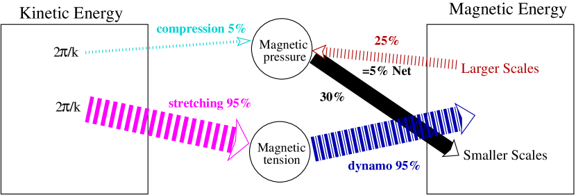
Figure 5: Net energy transfers in the kinematic phase. Work against magnetic tension, $T_{BKT}<0$ (stretching), accounts for 95% of magnetic energy generated while work against magnetic pressure, $T_{BKP}<0$ (compression), accounts for 5%. The latter is involved in the process of breaking down larger-scale field, $T_{KBP}<0$ (25%), into smaller-scale field, $T_{KBP}>0$ (30%), as part of the turbulent cascade. The dominant producer of magnetic energy is the stretching of magnetic field lines against the magnetic tension force, $T_{KBT}>0$ (associated with turbulent dynamo action).

In Figure 5, we illustrate the net energy transfers between kinetic and magnetic energies, and in Figure 6 we plot their scale dependence. We find that the dominant source (95%) of magnetic energy is the stretching of field lines against the magnetic tension force. A lesser source of magnetic energy (5%) is work against the magnetic pressure force. This latter energy is combined with larger-scale ($>30\,$km) magnetic energy lost (25%) to the “magnetic cascade” to produce (30%) smaller-scale ($<30\,$km) magnetic energy. Using a similar expression to Equation (2), we determine that the predominant scale at which fluid motions are doing work against the magnetic tension force to stretch magnetic field lines is $140\,$km. As seen in Figure 6 for Run 3, $-T_{BKT}$ peaks at the corresponding spatial frequency, $7\cdot 10^{-8}\,$cm^-1. Acceleration of large-scale fluid motions by the magnetic tension force, $T_{BKT}>0$ green dash-dotted line, shown in Figure 6 is mostly likely due to the somewhat artificial separation of the Lorentz force into magnetic tension and an isotropic magnetic pressure. As there is no Lorentz force along magnetic field lines, there can be no transfer along field lines and a portion of negative $T_{BKP}$ is offset by positive $T_{BKT}$. To see at which scales the magnetic field is gaining or losing energy, we examine $T_{KBT}$. We find that net magnetic energy is gained at all scales of the simulation. The predominant scale for magnetic energy production by stretching is identified as $65\,$km (a spatial frequency of $1.5\cdot 10^{-7}\,$cm^-1). Work against magnetic pressure, $T_{BKP}<0$ shown as a cyan dotted line, is mainly by granulation-scale fluid motions. The net result is to remove ($T_{KBP}<0$, red dotted line) larger-scale magnetic energy, which was produced by stretching motions, and break it down into smaller-scale magnetic structures ($T_{KBP}>0$, black solid line).

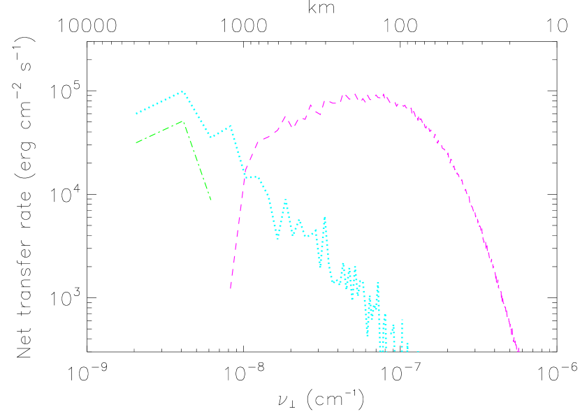
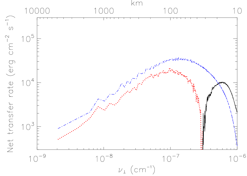
Figure 6: Net energy transfer rates for Run 3 versus horizontal spatial frequency, $\nu_{\perp}$, averaged over $t\in[11,28]\,$min (linear dynamo regime). Left: Work against magnetic tension, $T_{BKT}(k)<0$, is shown as pink dashed lines; fluid acceleration by magnetic tension, $T_{BKT}(k)>0$, as green dot-dashed; and work against magnetic pressure, $T_{BKP}(k)<0$, as cyan dotted. Right: Dynamo stretching, $T_{KBT}>0$, is shown as blue dot-dashed lines; generation by compression (and received from other scales), $T_{KBP}>0$, as black solid; and magnetic energy removed by compression, $T_{KBP}<0$ as red dotted. The error level of the transfer analysis is $2.5\cdot 10^{2}\,$erg cm^-2 s^-1 (see Appendix A.2).

With the sources of magnetic energy quantified on a scale-by-scale basis, we can now identify the source of the small-scale magnetic energy seen in Figure 4. This energy is seen to peak at scales between $60$ and $120\,$km. As we can see in Figure 6, the “cascade” dominates the production of magnetic energy only at scales below $20\,$km. Just as for incompressible turbulent dynamos (Mininni et al., 2005a), there exists a range of scales where the amplification of the magnetic field is dominated by injection of energy from turbulent stretching while the magnetic cascade dominates only at smaller scales. The source of the $\sim 100\,$km-scale magnetic energy is a dynamo process and not the turbulent tangling of larger-scale field lines. As the magnetic energy is predominantly produced at a scale of $65\,$km due to the stretching by fluid motions which operate predominately at a scale of $140\,$km (the peak of $-T_{BKT}$ in Figure 6), this suggests that the field lines stretched by these motions have a scale between $45$ and $120\,$km. This is due to the fact that all transfers occur between three fields whose wave-vectors must form a triad (see Figure 7). This allows us to rule out Alfvénic turbulent induction, i.e., small-scale velocity fluctuations interacting with a large-scale field to produce small-scale magnetic energy, as an important source of the small-scale magnetic energy in the simulations. Furthermore, as the three scales involved in the dynamo all lie in the inertial range, we can identify the MURaM dynamo as a turbulent small-scale dynamo.

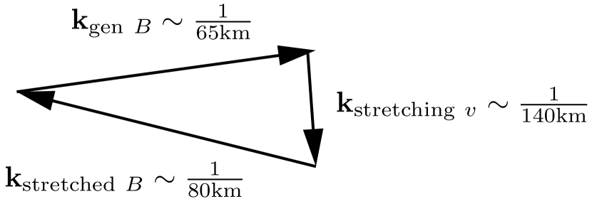
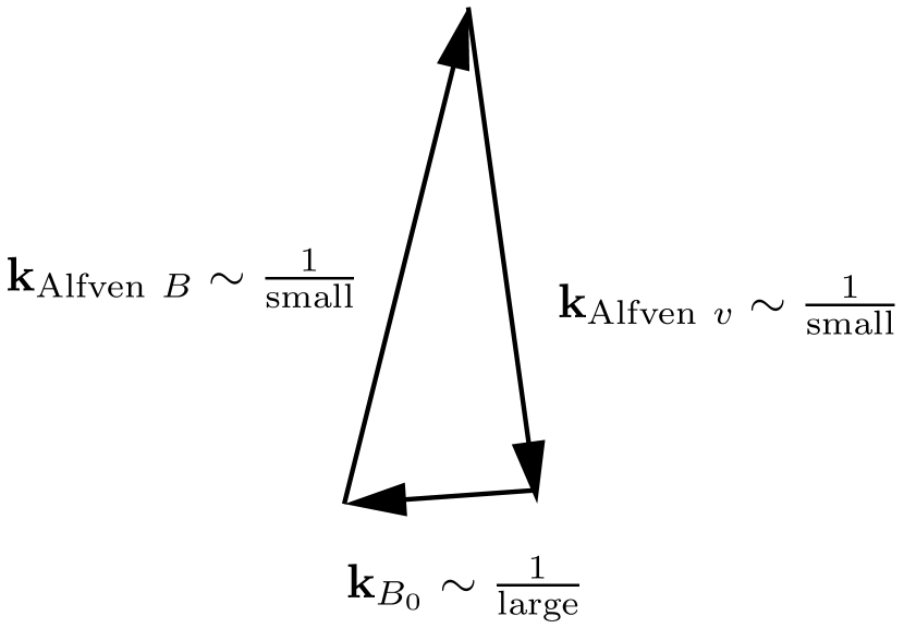
Figure 7: Illustration of triadic transfers. Left: Case for the linear phase of the MURaM dynamo Run 3. Fluid motions predominately at a scale of $\sim 140\,$km create magnetic energy predominately at a scale of $\sim 65\,$km. As the three wave-vectors must form a triad, the scale of the magnetic field being stretched must have a scale of $80\pm 40\,$km. Right: The Alfvénic case: small-scale velocity fluctuations interact with a large-scale field to produce small-scale magnetic energy.

For a small-scale dynamo, the smallest eddies provide the fastest stretching and this should be reflected in the transfer analysis. We would expect both the dominant scale of stretching motions and of magnetic field production to decrease as the Reynolds numbers are increased. That is, we expect the dynamo action to move to smaller and smaller scales. This is, in fact, what we find in the analysis. The dominant scale of stretching motions is $200\,$km for Run 1, $180\,$km for Run 2, and $140\,$km for Run 3 while the dominant scales of magnetic field production are $110\,$km, $100\,$km, and $65\,$km. This provides further evidence that the MURaM dynamo is a turbulent small-scale dynamo.

5 Nonlinear/saturated phase

The analysis of the nonlinear phase of the dynamo is quite similar to that already presented for the linear phase. For the sake of brevity, we describe only the differences between the two phases without figures. The magnetic energy spectra peak at scales slightly larger than the kinetic Taylor scales, $\lambda_{K}$. For scales larger than $\lambda_{K}$, a power-law $k_{\perp}^{\beta}$ with $\beta=0.4\pm 0.1$ can be fit. This is not as steep as in the linear regime and does not appear to be sensitive to the Reynolds number. It might be sensitive, however, to the large-scale flow geometry which will be investigated in a future work. There is a net transfer of energy, at 2% for Run 1 (4% for Run 2 and 8% for Run 3) of the total magnetic energy generation rate, to fluid motions via the magnetic tension force for scales smaller than $50\,$km. These are short-wavelength Alfvén waves. Magnetosonic waves are also produced, at 0.5% for Run 1 (1% for Run 2 and 2% for Run 3) of the magnetic energy generation rate, for scales smaller than $100\,$km. The saturation of the large-scale magnetic energy is reflected by a near balance of generation by stretching and losses to the compressive “cascade,” $T_{KBT}(k)+T_{KBP}(k)\approx 0$ for wavenumbers corresponding to scales above a few hundred km. We also note that the representative scale at which fluid motions are doing work against the magnetic tension force has increased, for Run 2, from the linear phase (where it is $180\,$km) up to $250\,$km. This result is similar to the result for an incompressible small-scale dynamo where in the saturated phase (as opposed to the linear phase), forcing-scale eddies dominate the energy injection as compared to turbulent eddies (Alexakis et al., 2005). The representative scale for the production of magnetic energy in Run 2 is $130\,$km in the saturated state. From triadic considerations, we expect that predominately magnetic field with scales between $85$ and $270\,$km is stretched. All results are again indicative of a small-scale turbulent dynamo as all scales in the triad are much smaller than the $\approx 1\,$Mm energy-containing scale of the granulation convection.

6 $P_{M}<1$

While our dynamo calculations include much of the physics believed to be present in the solar photosphere, the limited computational resources available today do not accommodate realistic values of the magnetic and kinetic Reynolds numbers. Moreover, the solar value of their ratio, the magnetic Prandtl number $\sim 10^{-5}$, will remain unachievable for strongly stratified, radiative small-scale dynamo simulations for many years to come. We can, however, take the first steps in this direction by employing the grid size of Run 3 with the magnetic diffusivity of Run 2. This run, Run 3-P (initialized from 15 minutes into Run 3 to reduce the computational expense) has $P_{M}\sim 0.8$ and an exponential growth rate of $\gamma\approx 1/1200\,$s^-1 (see Table 1 and Figure 1). The lower growth rate compared to Run 2 is likely due to a decreased ratio of $Re_{M}/Re_{M}^{C}$ ($Re_{M}^{C}$ increases with decreasing $P_{M}$, e.g., Schekochihin et al. 2005). The results of the transfer analysis are very similar to those shown in Figure 6. We identify the dominant scale of stretching motions as $150\,$km (close to that of Run 3) while the dominant scales of magnetic field production is $85\,$km (intermediary to Run 2 and Run 3). This indicates that the magnetic field being stretched has a scale of $130\pm 70\,$km. We conclude that the small-scale turbulent dynamo action is essentially unchanged in comparison to the runs with $P_{M}>1$.

7 Summary and Conclusions

We have determined that the MURaM surface dynamo is a turbulent small-scale dynamo. The dynamo growth rate, $\gamma$, increases with Reynolds number, consistent with the picture of dynamo action moving to smaller scales. At scales larger than the peak of magnetic energy, the magnetic spectrum is a power-law indicating a self-similar (e.g., turbulent) dynamo mechanism. The magnetic energy spectrum peaks at scales an order of magnitude smaller than the energy-containing scale of fluid motions (the granulation scale). This peak moves to smaller scales with increasing $Re_{M}$. By deriving spectral transfer analysis for anisotropic, compressible MHD, we are able to identify the source of this small-scale magnetic energy. The analysis ruled out two other possible mechanisms for the generation of the small-scale magnetic field: the tangling of larger-scale magnetic field lines associated with the turbulent cascade and Alfvénization of small-scale velocity fluctuations (or “turbulent induction”). We demonstrated that the source of the magnetic field was due, rather, to stretching motions in the inertial range of the turbulence. The inertial motions stretch predominantly small-scale magnetic field to produce more small-scale magnetic field. All three scales are significantly smaller than the granulation scale and move to even smaller scales with increasing Reynolds numbers. This positively identifies the dynamo process as a small-scale turbulent dynamo.

We also identified the key differences between the MURaM small-scale dynamo and those studied in the isotropic, incompressible MHD case. The presence of compressive motions opens up a new mechanism for the transfer of kinetic to magnetic energy. Namely, compression becomes involved in the “cascade” of magnetic energy to smaller scales, resulting in a net increase (summed over all scales) of magnetic energy. This mechanism accounts for only 5% of the rate of magnetic energy generated (and slightly decreasing with increasing $Re_{M}$). It is accomplished by Mm-scale fluid motions compressing larger scale magnetic structures (which are generated by stretching motions) into scales much smaller ($\lesssim 20\,$km) than the peak in the magnetic energy spectrum. This magnetic energy is then, presumably, dissipated by the magnetic diffusivity present in the simulations.

We have quantified the scale-dependent anisotropy of the fluid motions in our convection simulations via measurements of the second-order structure functions. The flow is anisotropic at scales larger than $50\,$km and this appears to play a role in the large-scale magnetic energy spectrum generated by the dynamo in that it differs from the isotropic Kazantsev result and varies with the degree of anisotropy of the flow. The slope is significantly less steep than the $k^{+3/2}$ law of the Kazantsev incompressible small-scale dynamo, but steepens with decreasing anisotropy of the flow as measured by the inertial-range velocity increments. This anisotropy decreases with Reynolds number as stronger horizontal fluctuations are generated by the turbulence (strong vertical fluctuations being induced by the convective driving).

Our analysis suggests that solar surface convection is capable, via a turbulent small-scale dynamo, of generating and sustaining small-scale magnetic field. Of course, dynamo action in the Sun will also be present in lower layers where more kinetic energy is available and where stratification and rotation may also lead to an inverse cascade to large scales ($\alpha-$effect). These two types of turbulent dynamos are likely intimately related. Even without a large-scale seed field local small-scale dynamo action should occur (e.g., during solar grand minima and for slowly rotating stars). In our simulation no large-scale background field is present. Turbulent induction of such a field (from a global dynamo) is an additional mechanism for the generation of small-scale field: it might obscure the presence of a small-scale dynamo. On the other hand, the large-scale magnetic field and the small-scale field produced from it will be subject to Ohmic decay: small-scale dynamo action might sustain magnetic field that would otherwise be lost. A future study should quantify at what background field strength the small-scale dynamo no longer dominates the production of small-scale magnetic field (as was done by Cattaneo et al. 2003 for the Boussinesq case).

The $P_{M}\ll 1$ case will remain inaccessible for a long time to come for “realistic” small-scale dynamo simulations of the solar surface. Nonetheless, evidence of the existence of $P_{M}\ll 1$ dynamos for idealistic simulations has now been given (Ponty et al., 2005). When possible, radiative MHD magneto-convection calculations for $P_{M}\lesssim 0.1$ should be carried out to determine if the magnetic field generated has a different morphology for this case. Differences in the magnetic structuring has been demonstrated for idealistic simulations of small-scale dynamo action with $P_{M}\lesssim 0.1$ (Iskakov et al., 2007; Schekochihin et al., 2007), but these differences likely only affect the solar magnetic field at sub-kilometer scales.

Small-scale dynamo action is not suppressed for $P_{M}\ll 1$ in idealistic simulations (Ponty et al., 2005; Iskakov et al., 2007; Schekochihin et al., 2007). We have shown that “realistic” simulations of dynamo action in strongly stratified, radiative MHD with partial ionization and little recirculation for $P_{M}\gtrsim 1$ (first achieved by Vögler & Schüssler 2007) also do not suppress the small-scale dynamo nor do they supplant it with another mechanism. It is reasonable, then, to infer that small-scale dynamo action can occur for $P_{M}\ll 1$ combined with solar-like stratification, radiation, ionization, and recirculation.

Acknowledgments

The authors would like to acknowledge fruitful discussions with A. Fournier, P. Mininni, W.-C. Müller, and D. Rosenberg. This work has been supported by the Max-Planck Society in the framework of the Interinstitutional Research Initiative “Turbulent transport and ion heating, reconnection and electron acceleration in solar and fusion plasmas” of the MPI for Solar System Research Lindau and the Institute for Plasma Physics, Garching (project MIF-IF-A-AERO8047).

Appendix A Appendix

A.1 Derivation of transfer functions

Transfer analysis for the incompressible case is well-known (see Kraichnan 1967 or for a more recent exposition, e.g., Alexakis et al. 2005). Here, we generalize the theory to the compressible and strongly stratified case. The latter requires a departure from the usual isotropic (and periodic) Fourier basis. Given a complete orthonormal basis, $\phi_{k}(\mathbf{x})$, and a function $g(\mathbf{x})$,

$$g(\mathbf{x})=\sum_{k}\hat{g}(k)\phi_{k}(\mathbf{x})$$ (A1)

with

$$\hat{g}(k)\equiv\int_{\Omega}g(\mathbf{x})\phi_{k}(\mathbf{x})dx^{3}$$ (A2)

where $\Omega$ is the analysis volume. Integrating the spatial density, $g(\mathbf{x})$, of a global quantity, $G$, over the volume allows us to identify $\hat{g}(k)$ as a “spectral density” of $G$ in $k$ space,

$$G\equiv\int_{\Omega}g(\mathbf{x})dx^{3}=\int_{\Omega}\sum_{k}\hat{g}(k)\phi_{k}(\mathbf{x})dx^{3}=\sum_{k}\hat{g}(k)\int_{\Omega}\phi_{k}(\mathbf{x})dx^{3}=\sum_{k}\hat{g}(k)\,.$$ (A3)

For example, the magnetic spectral energy density satisfies

$$E_{M}\equiv\int_{\Omega}e_{M}dx^{3}=\sum_{k}E_{M}(k)\,,$$ (A4)

where $e_{M}\equiv\frac{1}{8\pi}|\mathbf{B}|^{2}$ is the magnetic energy density (in Gaussian units) and $E_{M}$ is the total magnetic energy. From Parseval’s theorem we see that

$$\int_{\Omega}\mathbf{B}(\mathbf{x})\cdot\mathbf{B}(\mathbf{x})dx^{3}=\sum_{k}\hat{\mathbf{B}}(k)\cdot\hat{\mathbf{B}}^{\ast}(k)$$ (A5)

where $\cdot^{\ast}$ specifies conjugate (depending on the basis). This allows us to identify that the magnetic spectral energy density is

$$E_{M}(k)\equiv\frac{1}{8\pi}\hat{\mathbf{B}}(k)\cdot\hat{\mathbf{B}}^{\ast}(k)\,.$$ (A6)

We can derive its temporal evolution (the magnetic component of the energy balance equation) by projecting the induction equation,

$$\partial_{t}\mathbf{B}+\mathbf{v}\cdot\nabla\mathbf{B}=\mathbf{B}\cdot\nabla\mathbf{v}-\mathbf{B}\nabla\cdot\mathbf{v}+\eta\nabla^{2}\mathbf{B}\,,$$ (A7)

onto the basis functions and then taking the dot product of this expression with $\frac{1}{4\pi}\hat{\mathbf{B}}^{\ast}(k)$. We add the conjugate of the result and divide the sum by two to derive that the time evolution of the spectral magnetic energy density,

$$\frac{d}{dt}E_{M}(k)={T_{KB}(k)+T_{IB}(k)}\,,$$ (A8)

is given by the magnetic energy transfer functions (representing the transfer of magnetic energy in $k-$space). In general, the transfer functions, $T_{XY}(k)$, measure the rate of energy transfer from energy reservoir $X$ to the $k-$component of reservoir $Y$ (also the work done on field $Y$ by field $X$ at wavenumber $k$). For $T_{XY}(k)>0$ ($<0$) energy is received (lost) by the $k-$component of $Y$. In particular, $T_{KB}(k)\equiv T_{KBT}(k)+T_{KBP}(k)$ denotes the energy transfer rate from the kinetic energy reservoir to the $k-$component of the magnetic energy reservoir through the dynamo term (stretching against the magnetic tension force),

$${T_{KBT}(k)}=\frac{1}{4\pi}\hat{\mathbf{B}}(k)\cdot\widehat{\left[\mathbf{B}\cdot\nabla\mathbf{v}\right]}^{\ast}(k)\,,$$ (A9)

and compression against magnetic pressure,

$${T_{KBP}(k)=-\frac{1}{4\pi}\hat{\mathbf{B}}(k)\cdot\widehat{\left[\mathbf{B}\nabla\cdot\mathbf{v}\right]}^{\ast}(k)-\frac{1}{4\pi}\hat{\mathbf{B}}(k)\cdot\widehat{\left[\mathbf{v}\cdot\nabla\mathbf{B}\right]}^{\ast}(k)}\,.$$ (A10)

$T_{IB}(k)$ represents the (negative of) energy loss rate to Joule heating,

$$T_{IB}(k)=\frac{\eta}{4\pi}\hat{\mathbf{B}}(k)\cdot\widehat{\left[\nabla^{2}\mathbf{B}\right]}^{\ast}(k)\,.$$ (A11)

The kinetic spectral energy density can be expressed

$$E_{K}(k)=\frac{1}{4}\left(\hat{\mathbf{v}}(k)\cdot\widehat{\left[\rho\mathbf{v}\right]}^{\ast}(k)+\widehat{\left[\rho\mathbf{v}\right]}(k)\cdot\hat{\mathbf{v}}^{\ast}(k)\right)\,.$$ (A12)

Note that this is different from the velocity spectrum,

$$E_{V}(k)=\frac{1}{2}\hat{\mathbf{v}}(k)\cdot\hat{\mathbf{v}}^{\ast}(k)\,,$$ (A13)

in the incompressible theory of Kolmogorov (see, e.g., Frisch 1995). The time evolution of the kinetic spectral energy density is given by

$$\frac{d}{dt}E_{K}(k)=\frac{1}{2}\hat{\mathbf{v}}(k)\cdot\partial_{t}\widehat{\left[\rho\mathbf{v}\right]}^{\ast}(k)+\frac{1}{2}\widehat{\left[\rho\mathbf{v}\right]}^{\ast}(k)\cdot\partial_{t}\hat{\mathbf{v}}(k)\,.$$ (A14)

This is an alternative expression to the one derived by Miura & Kida (1995) for the non-magnetic case. The kinetic energy transfer functions can be derived similarly to the expression for the magnetic transfer utilizing the conservation of momentum density equation, (see, e.g., Vögler et al. 2005),

$$\partial_{t}(\rho\mathbf{v})+\nabla\cdot(\rho\mathbf{v}\mathbf{v})=-\nabla P+\rho\mathbf{F}+\mu\nabla\cdot\uuline{\tau}+\frac{1}{c}(\mathbf{J}\times\mathbf{B})\,,$$ (A15)

and the conservation of mass density, $\rho$,

$$\partial_{t}\rho+\nabla\cdot(\rho\mathbf{v})=0\,,$$ (A16)

which can be combined to form the momentum equation in terms of the velocity

$$\partial_{t}\mathbf{v}+\mathbf{v}\cdot\nabla\mathbf{v}=-\frac{1}{\rho}\nabla P+\mathbf{F}+\frac{\mu}{\rho}\nabla\cdot\uuline{\tau}+\frac{1}{\rho c}(\mathbf{J}\times\mathbf{B})\,.$$ (A17)

Taking the appropriate dot products and integrating over the total volume, we derive that the kinetic part of the energy balance equation,

$${\frac{d}{dt}E_{K}(k)=\mathfrak{f}(k)+T_{KK}(k)+T_{BK}(k)+T_{IK}(k)}$$ (A18)

is given by the energy injection into the volume by body forces

$${\mathfrak{f}(k)=\frac{1}{2}\hat{\mathbf{v}}(k)\cdot\widehat{\left[\rho\mathbf{F}\right]}^{\ast}(k)+\frac{1}{2}\widehat{\left[\rho\mathbf{v}\right]}^{\ast}(k)\cdot\hat{\mathbf{F}}(k)}$$ (A19)

and the sum of the kinetic energy transfer functions. $T_{KK}(k)=T_{KKA}(k)+T_{KKC}(k)$ is the transfer of kinetic energy inside the kinetic energy reservoir (“cascade”), by advection

$$T_{KKA}(k)=-\frac{1}{2}\hat{\mathbf{v}}(k)\cdot\widehat{\left[\mathbf{v}\cdot\nabla(\rho\mathbf{v})\right]}^{\ast}(k)-\frac{1}{2}\widehat{\left[\rho\mathbf{v}\right]}^{\ast}(k)\cdot\widehat{\left[\mathbf{v}\cdot\nabla\mathbf{v}\right]}(k)\,,$$ (A20)

and compressible (irrotational) motions

$$T_{KKC}(k)=-\frac{1}{2}\hat{\mathbf{v}}(k)\cdot\widehat{\left[\rho\mathbf{v}\nabla\cdot\mathbf{v}\right]}^{\ast}(k)\,.$$ (A21)

$T_{IK}(k)=T_{IKC}(k)+T_{IKD}(k)$ represents energy transferred from the internal energy reservoir to the kinetic energy reservoir by compression,

$$T_{IKC}(k)=-\frac{1}{2}\hat{\mathbf{v}}(k)\cdot\widehat{\left[\nabla P\right]}^{\ast}(k)-\frac{1}{2}\widehat{\left[\rho\mathbf{v}\right]}^{\ast}(k)\cdot\widehat{\left[\frac{1}{\rho}\nabla P\right]}(k)\,,$$ (A22)

and viscous dissipation,

$$T_{IKD}(k)=-\frac{1}{2}\hat{\mathbf{v}}(k)\cdot\widehat{\left[\mu\nabla\cdot\uuline{\tau}\right]}^{\ast}(k)-\frac{1}{2}\widehat{\left[\rho\mathbf{v}\right]}^{\ast}(k)\cdot\widehat{\left[\frac{\mu}{\rho}\nabla\cdot\uuline{\tau}\right]}(k)\,.$$ (A23)

$T_{BK}(k)=T_{BKT}(k)+T_{BKP}(k)$ represents energy transferred from the magnetic energy reservoir to the kinetic energy reservoir by the work of the Lorenz force both via magnetic tension,

$$T_{BKT}(k)=\frac{1}{8\pi}\hat{\mathbf{v}}(k)\cdot\widehat{\left[\mathbf{B}\cdot\nabla\mathbf{B}\right]}^{\ast}(k)+\frac{1}{8\pi}\widehat{\left[\rho\mathbf{v}\right]}^{\ast}(k)\cdot\widehat{\left[\frac{1}{\rho}\mathbf{B}\cdot\nabla\mathbf{B}\right]}(k)$$ (A24)

and via magnetic pressure,

$$T_{BKP}(k)=\frac{1}{8\pi}\hat{\mathbf{v}}(k)\cdot\widehat{\left[-\frac{1}{2}\nabla|\mathbf{B}|^{2}\right]}^{\ast}(k)+\frac{1}{8\pi}\widehat{\left[\rho\mathbf{v}\right]}^{\ast}(k)\cdot\widehat{\left[-\frac{1}{2\rho}\nabla|\mathbf{B}|^{2}\right]}(k)\,.$$ (A25)

For an ideal gas with adiabatic index, $\gamma$, the internal energy density is given by $e_{I}=P/(\gamma-1)$ and the pressure is given by $P=\rho\mathfrak{R}T$ where $T$ is the temperature and $\mathfrak{R}$ the gas constant. The internal spectral energy density can then be expressed

$$E_{I}(k)=\frac{\mathfrak{R}}{2(\gamma-1)}\left(\hat{T}(k)\hat{\rho}^{\ast}(k)+\hat{\rho}(k)\hat{T}^{\ast}(k)\right)\,.$$ (A26)

The time evolution of the internal spectral energy density is then

$$\frac{d}{dt}E_{I}(k)=\frac{\mathfrak{R}}{\gamma-1}\hat{T}(k)\partial_{t}\hat{\rho}^{\ast}(k)+\frac{\mathfrak{R}}{\gamma-1}\hat{\rho}^{\ast}(k)\partial_{t}\hat{T}(k)\,.$$ (A27)

Using the conservation of mass, Equation (A16), and the energy equation for temperature,

$$\rho\frac{\mathfrak{R}}{\gamma-1}\left(\partial_{t}T+\mathbf{v}\cdot\nabla T\right)=\nabla\cdot(\kappa\nabla T)-P\nabla\cdot\mathbf{v}+Q_{rad}+\mu(\uuline{\tau}\cdot\nabla)^{\top}\mathbf{v}\\ +(\frac{c}{4\pi})^{2}\frac{1}{\sigma}|\mathbf{J}|^{2}\,,$$

we find the that time evolution of the internal spectral energy density,

$$\frac{d}{dt}E_{I}(k)=\mathfrak{f}_{I}(k)+T_{I}(k)\,,$$ (A28)

is given by the radiative heating (cooling), $\sum_{k}\mathfrak{f}_{I}(k)=\int_{\Omega}Q_{rad}dx^{3}$, and the sum of the internal energy transfer function, $T_{I}(k)$. $T_{I}(k)=T_{II}(k)+T_{KI}(k)+T_{BI}(k)$. $T_{II}(k)$ is the transfer of internal energy inside the internal energy reservoir: $T_{II}(k)=-\frac{\mathfrak{R}}{\gamma-1}\hat{T}(k)\widehat{\left[\nabla\cdot(\rho\mathbf{v})\right]}^{\ast}(k)-\frac{\mathfrak{R}}{\gamma-1}\hat{\rho}^{\ast}(k)\widehat{\left[\mathbf{v}\cdot\nabla T\right]}(k)+\hat{\rho}^{\ast}(k)\widehat{\left[\frac{1}{\rho}\nabla\cdot(\kappa\nabla T)\right]}(k)$. $T_{KI}(k)=T_{KIC}(k)+T_{KID}(k)$ represents transfer of kinetic energy to internal energy by work against pressure gradients, $T_{KIC}(k)=-\hat{\rho}^{\ast}(k)\widehat{\left[\frac{1}{\rho}P\nabla\cdot\mathbf{v}\right]}(k)$ and viscous dissipation, $T_{KID}(k)=\hat{\rho}^{\ast}(k)\widehat{\left[\frac{1}{\rho}\mu(\uuline{\tau}\cdot\nabla)^{\top}\mathbf{v}\right]}(k)$. $T_{BI}(k)$ represents transfer of magnetic energy to internal energy by Joule heating, $T_{BI}(k)=\hat{\rho}^{\ast}(k)\widehat{\left[\frac{1}{\rho}(\frac{c}{4\pi})^{2}\frac{1}{\sigma}|\mathbf{J}|^{2}\right]}(k)$ where

$$\sum_{k}T_{IB}(k)+T_{BI}(k)=-(\frac{c}{4\pi})\frac{1}{\sigma}\int_{\Omega}\nabla\cdot\left(\mathbf{J}\times\mathbf{B}\right)dx^{3}\,.$$ (A29)

As this is the integral over a divergence term, we recognize that the magnetic energy lost and the Joule heat gained differ only by a surface term. The sum of transfers between kinetic and magnetic energies is

$$\sum_{k}T_{KB}(k)+T_{BK}(k)=\frac{1}{4\pi}\int_{\Omega}\nabla\cdot\left((\mathbf{v}\times\mathbf{B})\times\mathbf{B}\right)dx^{3}{\equiv\mathfrak{P}_{\partial\Omega}\,,}$$ (A30)

where $\mathfrak{P}_{\partial\Omega}$ is the inductive component of the Poynting flux into the domain. From this, we see that the time derivative of the total magnetic energy,

$$\frac{d}{dt}E_{M}=\sum_{k}T_{B}(k)=\mathfrak{p}_{\partial\Omega}-\sum_{k}T_{BK}(k)-\sum_{k}T_{BI}(k)\,,$$ (A31)

is given by the inflow of electromagnetic energy (negative Poynting flux) at the boundary, $\partial\Omega$,

$$\mathfrak{p}_{\partial\Omega}=-\frac{c}{4\pi}\int_{\Omega}\nabla\cdot\left(\mathbf{E}\times\mathbf{B}\right)dx^{3}=\int_{\partial\Omega}-\frac{c}{4\pi}\left(\mathbf{E}\times\mathbf{B}\right)\cdot d\mathbf{A}\,,$$ (A32)

the Lorentz force work against internal fluid motions, $\sum_{k}T_{BK}(k)$, and diffusive losses to Joule heating, $\sum_{k}T_{BI}(k)$.

The right hand side of Equation (A30) is equivalent to a surface term via Gauss’s divergence theorem,

$$\mathfrak{P}_{\partial\Omega}\equiv\frac{1}{4\pi}\int_{\partial\Omega}\left((\mathbf{v}\times\mathbf{B})\times\mathbf{B}\right)\cdot d\mathbf{A}\,.$$ (A33)

This surface term is zero for common choices of boundary conditions, hence,

$$\sum_{k}T_{KB}(k)=-\sum_{k}T_{BK}(k)\,.$$ (A34)

This follows from the fact that $T_{KB}$ and $T_{BK}$ measure the transfer of energy between the magnetic and kinetic energy reservoirs. We can also show that

$$\sum_{k}T_{KBP}(k)+T_{BKP}(k)=\frac{1}{4\pi}\int_{\partial\Omega}|\mathbf{B}|^{2}\mathbf{v}\cdot d\mathbf{A}\,.$$ (A35)

This is another surface term and

$$\sum_{k}T_{KBP}(k)=-\sum_{k}T_{BKP}(k)$$ (A36)

as these two functions measure energy transfer via the interaction of compression and magnetic pressure. In incompressible MHD, the second term of $T_{KBP}$ in Equation (A10), that is

$$T_{BB}(k)=-\frac{1}{4\pi}\hat{\mathbf{B}}(k)\cdot\widehat{\left[\mathbf{v}\cdot\nabla\mathbf{B}\right]}^{\ast}(k)\,,$$ (A37)

is identified as the transfer rate of magnetic energy to other scales within the magnetic energy reservoir (the magnetic energy “cascade”). As the first term of $T_{KBP}$ is identically zero and $\sum_{k}T_{BKP}(k)=0$ for incompressible flow, $\sum_{k}T_{BB}(k)=0$ (transfer is internal to magnetic energy reservoir). This is not true for compressible flow and the magnetic “cascade” cannot be separated from compressive kinetic energy transfers. From Equations (A34) and (A36), we also find

$$\sum_{k}T_{KBT}(k)=-\sum_{k}T_{BKT}(k)\,,$$ (A38)

as that these two functions measure energy transfer via the stretching of magnetic field lines against the magnetic tension force. A similar analysis shows, $\sum_{k}T_{IB}(k)=-\sum_{k}T_{BI}(k)$, $\sum_{k}T_{IKD}(k)=-\sum_{k}T_{KID}(k)$, and $\sum_{k}T_{IKC}(k)=-\sum_{k}T_{KIC}(k)$.

A.2 Application to MURaM simulations

For stratified convection, we use as the orthonormal basis functions a two-dimensional Fourier basis multiplied by vertical cardinal basis functions,

$$\phi_{k_{x},k_{y},z^{\prime}}=\frac{1}{2\pi}e^{-i(k_{x}x+k_{y}y)}\delta(z-z^{\prime})\,.$$ (A39)

To study the generation (or loss of) magnetic energy at a given scale, the resulting transfer functions are projected onto a one-dimensional wavenumber, $k_{{\perp}}^{2}=k_{x}^{2}+k_{y}^{2}$, and summed over the vertical direction,

$$T_{KB}(k_{{\perp}})\equiv\sum_{z}\sum_{k_{{\perp}}=\sqrt{k_{x}^{2}+k_{y}^{2}}}T_{KB}(k_{x},k_{y},z)\,.$$ (A40)

To quantify the source of magnetic energy generation at the scale $2\pi/k_{\perp}$, we need only measure $T_{KBT}$ and $T_{KBP}$. The resistive transfer, $T_{IB}$, mostly serves as a sink for magnetic energy at small ($\lesssim 5\Delta x$) scales. To complete the physical picture, we also measure $T_{BKT}$ and $T_{BKP}$, the rate at which kinetic energy is lost to (gained from) the magnetic field. Transfers between internal and kinetic energies may be ignored as we are only interested in generation and loss of magnetic energy in a dynamo analysis. As shown in the previous section, Equation (A30), the sum of these four transfers is equal to the inflow of electromagnetic energy from the inductive component of the Poynting flux, $\mathfrak{P}_{\partial\Omega}$, into the domain,

$$\sum_{z_{bot}<z<z_{top}}\sum_{k_{{\perp}}}T_{KBT}+T_{KBP}+T_{BKT}+T_{BKP}+T_{MM}+\Delta_{chain}=\mathfrak{P}_{\partial\Omega}\,.$$ (A41)

Here $T_{MM}(k)=\frac{1}{4\pi}\hat{\mathbf{B}}(k)\cdot\widehat{\left[\mathbf{v}\nabla\cdot\mathbf{B}\right]}^{\ast}(k)$ denotes the influence of the numerical artifacts of magnetic monopoles and

$$\Delta_{chain}\equiv\int_{\Omega}\mathbf{v}\cdot\nabla e_{M}-\frac{1}{4\pi}\mathbf{B}\cdot\left(\mathbf{v}\cdot\nabla\mathbf{B}\right)dx^{3}$$ (A42)

arises because of numerical inaccuracies in the chain rule, $0.5dB^{2}/dx=BdB/dx$. Multiplying MURaM’s 5-pt stencil for the derivative of $B$ by $B$ yields,

$$B\frac{dB}{dx}-\frac{\Delta x^{4}}{30}BB^{(5)}\,,$$ (A43)

while the numerical derivative of $B^{2}/2$ yields

$$B\frac{dB}{dx}-\frac{\Delta x^{4}}{36}(6\frac{dB}{dx}B^{(4)}+12\frac{d^{2}B}{dx^{2}}B^{(3)}+5B^{(3)}B^{(4)})\,.$$ (A44)

As strong gradients of the magnetic field exist in the downflows, $o(B)\ll o(B^{(n)})$ and significant departures, $\approx 8\%$ of the total transfer rate, from the chain rule occur. We track this through direct calculation of $\Delta_{chain}$. Lower order errors occur for the two grid points closest to the top and bottom boundaries. For this reason we choose our analysis domain such that the boundary, $\partial\Omega$, is halfway between the second and third grid points from the bottom (and top). $\mathfrak{P}_{\partial\Omega}$ is interpolated using Newton divided differences and the error in calculating Equation (A41) is computed for each snapshot. As Equation (A42) accounts for the chain-rule error only for the largest and most easily calculated contribution, some small residual error is found. This error, always less than 3%, is assumed to be spread equally over $k_{\perp}-$space and is reported for all plots of transfer functions.

References

- Alexakis et al. (2005) Alexakis, A., Mininni, P. D., & Pouquet, A. 2005, Phys. Rev. E, 72, 046301
- Batchelor (1950) Batchelor, G. K. 1950, Proceedings of the Royal Society of London. Series A, Mathematical and Physical Sciences, 201, 405
- Batchelor (1953) —. 1953, Theory of Homogeneous Turbulence (Cambridge, England: Cambridge University Press)
- Boldyrev & Cattaneo (2004) Boldyrev, S. & Cattaneo, F. 2004, Physical Review Letters, 92, 144501
- Brun et al. (2004) Brun, A. S., Miesch, M. S., & Toomre, J. 2004, ApJ, 614, 1073
- Cattaneo (1999) Cattaneo, F. 1999, ApJ, 515, L39
- Cattaneo et al. (2003) Cattaneo, F., Emonet, T., & Weiss, N. 2003, ApJ, 588, 1183
- Covas et al. (1997) Covas, E., Tworkowski, A., Brandenburg, A., & Tavakol, R. 1997, A&A, 317, 610
- Debliquy et al. (2005) Debliquy, O., Verma, M. K., & Carati, D. 2005, Physics of Plasmas, 12, 042309
- Eyink (2006) Eyink, G. L. 2006, Journal of Fluid Mechanics, 549, 191
- Field & Blackman (2002) Field, G. B. & Blackman, E. G. 2002, ApJ, 572, 685
- Field et al. (1999) Field, G. B., Blackman, E. G., & Chou, H. 1999, ApJ, 513, 638
- Frisch (1995) Frisch, U. 1995, Turbulence, The Legacy of A. N. Kolmogorov (Cambridge, UK: Cambridge University Press)
- Gómez et al. (2005a) Gómez, D. O., Mininni, P. D., & Dmitruk, P. 2005a, Advances in Space Research, 35, 899
- Gómez et al. (2005b) —. 2005b, Physica Scripta Volume T, 116, 123
- Hagenaar et al. (2003) Hagenaar, H. J., Schrijver, C. J., & Title, A. M. 2003, ApJ, 584, 1107
- Haugen & Brandenburg (2004) Haugen, N. E. L. & Brandenburg, A. 2004, Phys. Rev. E, 70, 036408
- Iskakov et al. (2007) Iskakov, A. B., Schekochihin, A. A., Cowley, S. C., McWilliams, J. C., & Proctor, M. R. E. 2007, Physical Review Letters, 98, 208501
- Kraichnan (1967) Kraichnan, R. H. 1967, Physics of Fluids, 10, 1417
- Kraichnan (1971) —. 1971, Journal of Fluid Mechanics, 47, 525
- Krause & Raedler (1980) Krause, F. & Raedler, K. H. 1980, Mean-field magnetohydrodynamics and dynamo theory, ed. K. H. Krause, F. & Raedler
- Maltrud & Vallis (1993) Maltrud, M. E. & Vallis, G. K. 1993, Physics of Fluids, 5, 1760
- Meneguzzi et al. (1981) Meneguzzi, M., Frisch, U., & Pouquet, A. 1981, Physical Review Letters, 47, 1060
- Mininni et al. (2005a) Mininni, P., Alexakis, A., & Pouquet, A. 2005a, Phys. Rev. E, 72, 046302
- Mininni et al. (2008) Mininni, P. D., Alexakis, A., & Pouquet, A. 2008, Phys. Rev. E, 77, 036306
- Mininni et al. (2005b) Mininni, P. D., Ponty, Y., Montgomery, D. C., Pinton, J.-F., Politano, H., & Pouquet, A. 2005b, ApJ, 626, 853
- Miura & Kida (1995) Miura, H. & Kida, S. 1995, Physics of Fluids, 7, 1732
- Monchaux et al. (2009) Monchaux, R., Berhanu, M., Aumaître, S., Chiffaudel, A., Daviaud, F., Dubrulle, B., Ravelet, F., Fauve, S., Mordant, N., Pétrélis, F., Bourgoin, M., Odier, P., Pinton, J., Plihon, N., & Volk, R. 2009, Physics of Fluids, 21, 035108
- Monchaux et al. (2007) Monchaux, R., Berhanu, M., Bourgoin, M., Moulin, M., Odier, P., Pinton, J.-F., Volk, R., Fauve, S., Mordant, N., Pétrélis, F., Chiffaudel, A., Daviaud, F., Dubrulle, B., Gasquet, C., Marié, L., & Ravelet, F. 2007, Physical Review Letters, 98, 044502
- Ossendrijver (2003) Ossendrijver, M. 2003, A&A Rev., 11, 287
- Petrovay & Szakaly (1993) Petrovay, K. & Szakaly, G. 1993, A&A, 274, 543
- Pietarila Graham et al. (2009) Pietarila Graham, J., Danilovic, S., & Schüssler, M. 2009, ApJ, 693, 1728
- Ponty et al. (2005) Ponty, Y., Mininni, P. D., Montgomery, D. C., Pinton, J.-F., Politano, H., & Pouquet, A. 2005, Physical Review Letters, 94, 164502
- Ponty et al. (2007) Ponty, Y., Mininni, P. D., Pinton, J.-F., Politano, H., & Pouquet, A. 2007, New Journal of Physics, 9, 296
- Pouquet et al. (1976) Pouquet, A., Frisch, U., & Leorat, J. 1976, Journal of Fluid Mechanics, 77, 321
- Rogachevskii & Kleeorin (1997) Rogachevskii, I. & Kleeorin, N. 1997, Phys. Rev. E, 56, 417
- Sánchez Almeida (2003) Sánchez Almeida, J. 2003, A&A, 411, 615
- Sánchez Almeida (2004) Sánchez Almeida, J. 2004, in ASP Conf. Ser. 325: The Solar-B Mission and the Forefront of Solar Physics, ed. T. Sakurai & T. Sekii, 115–+
- Sánchez Almeida et al. (2003) Sánchez Almeida, J., Emonet, T., & Cattaneo, F. 2003, in Astronomical Society of the Pacific Conference Series, Vol. 307, Astronomical Society of the Pacific Conference Series, ed. J. Trujillo-Bueno & J. Sanchez Almeida, 293–+
- Schekochihin et al. (2004) Schekochihin, A. A., Cowley, S. C., Taylor, S. F., Maron, J. L., & McWilliams, J. C. 2004, ApJ, 612, 276
- Schekochihin et al. (2005) Schekochihin, A. A., Haugen, N. E. L., Brandenburg, A., Cowley, S. C., Maron, J. L., & McWilliams, J. C. 2005, ApJ, 625, L115
- Schekochihin et al. (2007) Schekochihin, A. A., Iskakov, A. B., Cowley, S. C., McWilliams, J. C., Proctor, M. R. E., & Yousef, T. A. 2007, New Journal of Physics, 9, 300
- Stein et al. (2003) Stein, R. F., Bercik, D., & Nordlund, Å. 2003, in Astronomical Society of the Pacific Conference Series, Vol. 286, Current Theoretical Models and Future High Resolution Solar Observations: Preparing for ATST, ed. A. A. Pevtsov & H. Uitenbroek, 121–+
- Title & Schrijver (1998) Title, A. M. & Schrijver, C. J. 1998, in Astronomical Society of the Pacific Conference Series, Vol. 154, Cool Stars, Stellar Systems, and the Sun, ed. R. A. Donahue & J. A. Bookbinder, 345–+
- Trujillo Bueno et al. (2004) Trujillo Bueno, J., Shchukina, N., & Asensio Ramos, A. 2004, Nature, 430, 326
- Verma et al. (2005) Verma, M. K., Ayyer, A., & Chandra, A. V. 2005, Physics of Plasmas, 12, 082307
- Vögler (2003) Vögler, A. 2003, PhD thesis, Göttingen University
- Vögler & Schüssler (2007) Vögler, A. & Schüssler, M. 2007, A&A, 465, L43
- Vögler et al. (2005) Vögler, A., Shelyag, S., Schüssler, M., Cattaneo, F., Emonet, T., & Linde, T. 2005, A&A, 429, 335
- Weygand et al. (2007) Weygand, J. M., Matthaeus, W. H., Dasso, S., Kivelson, M. G., & Walker, R. J. 2007, Journal of Geophysical Research (Space Physics), 112, 10201
- Zhou (1993) Zhou, Y. 1993, Physics of Fluids, 5, 1092