Selecting Quasars by their Intrinsic Variability
Abstract
We present a new and simple technique for selecting extensive, complete and pure quasar samples, based on their intrinsic variability. We parametrize the single-band variability by a power-law model for the light-curve structure function, with amplitude and power-law index . We show that quasars can be efficiently separated from other non-variable and variable sources by the location of the individual sources in the - plane. We use 60 epochs of imaging data, taken over 5 years, from the SDSS stripe 82 (S82) survey, where extensive spectroscopy provides a reference sample of quasars, to demonstrate the power of variability as a quasar classifier in multi-epoch surveys. For UV-excess selected objects, variability performs just as well as the standard SDSS color selection, identifying quasars with a completeness of 90% and a purity of 95%. In the redshift range , where color selection is known to be problematic, variability can select quasars with a completeness of 90% and a purity of 96%. This is a factor of 5-10 times more pure than existing color-selection of quasars in this redshift range. Selecting objects from a broad color box without -band information, variability selection in S82 can afford completeness and purity of 92%, despite a factor of 30 more contaminants than quasars in the color-selected feeder sample. This confirms that the fraction of quasars hidden in the “stellar locus” of color-space is small. To test variability selection in the context of Pan-STARRS 1 (PS1) we created mock PS1 data by down-sampling the S82 data to just 6 epochs over 3 years. Even with this much sparser time sampling, variability is an encouragingly efficient classifier. For instance, a 92% pure and 44% complete quasar candidate sample is attainable from the above -selected catalog. Finally, we show that the presented - technique, besides selecting clean and pure samples of quasars (which are stochastically varying objects), is also efficient at selecting (periodic) variable objects such as RR Lyrae.
Subject headings:
methods: observational – surveys – galaxies:quasars:general1. Introduction
Large, complete and pure samples of quasars have proven crucial for observational cosmology. Quasars serve as probes of galaxy evolution, map black hole growth and probe (and affect) the intergalactic medium. Quasar clustering is a tracer of mass clustering on both large and small scales (Croom et al., 2005, 2009b; Shen et al., 2007, 2009; Ross et al., 2009), and the large samples provide precise measurements of the evolution and spectral properties of the quasars themselves (Vanden Berk et al., 2001; Richards et al., 2002b, 2004, 2006, 2009; Boyle et al., 2000; Croom et al., 2009b). Furthermore, huge quasar samples are required to find a large number of gravitationally lensed quasars (Oguri et al., 2006; Inada et al., 2008). Through the gravitationally magnified quasars the quasar samples indirectly contribute to the understanding of the molecular gas content in distant galaxies (Yun et al., 1997; Riechers, 2007a, b), mapping of the intergalactic medium and structures (e.g. Metcalf, 2005; Hennawi et al., 2006b; Hennawi & Prochaska, 2007) and exploration of the dark matter (halo) content of galaxies (Dalal & Kochanek, 2002; Bradač et al., 2002; Dobler & Keeton, 2006; Macciò, 2008). In short, large well-defined quasar samples are a cornerstone of observational cosmology.
Photometric quasar samples have recently grown to nearly a million objects (850,000 actual quasars; Richards et al., 2009). Despite these impressive catalog sizes the number statistics still limit the achievable science in various cases; especially those where particular and hence rare geometric constellations of quasars are needed. For instance a 3 detection of a luminosity-dependent quasar bias above 1.9 when analyzing the angular clustering of quasars, needs an estimated sample size of at least 1,200,000 actual quasars (Myers et al., 2007a, b; Myers, White & Ball, 2009). Searches for binary quasars (Hennawi et al., 2006b, 2009; Myers et al., 2008) - which provide interesting knowledge about small scale clustering and hence shed light on quasar triggering mechanisms and the nature of quasar progenitors - also should be based on samples with actual quasars in order to obtain reasonably sized statistical samples of possible quasar pairs. Also quasar-galaxy clustering (e.g. Scranton et al., 2005; Lopez et al., 2008; Padmanabhan et al., 2008; Burbidge & Napier, 2009), i.e. exploring the statistics of quasars behind the foreground galaxies, calls for larger (relatively low-) quasar samples than exist to date. Furthermore, exploring the ”transverse proximity effect” in the Ly forest of quasars, with foreground quasars near the sight line of background quasars (e.g. Hennawi et al., 2006a; Hennawi & Prochaska, 2007) is presently limited by quasar sample sizes. Obtaining larger photometric quasar catalogs to boost possible candidates for spectroscopic follow-up is needed. The 3 detections of the integrated Sachs-Wolfe effect by cross correlating quasars with the CMB to estimate the size of cosmological parameters and the dark energy equation of state (e.g. Giannantonio et al., 2008; Xia et al., 2009; Scranton et al., 2005) will also be improved by larger photometric samples of 15 quasars. Last but not least, larger photometric quasar catalogs will enhance the number of known gravitationally lensed quasars (e.g. Oguri & Marshall, 2010). At present 100 quasar lenses are known and an even larger sample of the relatively rare gravitationally lensed quasar systems will among other things improve our knowledge about cosmology, galaxy mass distributions, quasar hosts and the growth of the host’s central black holes (Schneider, Kochanek & Wambsganss, 2006, and references therein). These few examples serve as a scientific justification for pursuing even larger photometric samples of low as well as of high redshift quasars.
Most existing large quasar samples haven been selected on the basis of their UV/optical colors or radio flux. However, quasars are known to vary intrinsically on timescales of months to years and can therefore be selected alternatively on the basis of their variability (alone). Several physical processes are discussed as important causes of this variability: foremost are accretion disc instabilities (Rees, 1984; Kawaguchi et al., 1998; Pereyra et al., 2006) but also large-scale changes in the amount of in-falling material may be important (e.g. Hopkins et al., 2006, and references therein). Also, starbursts in the host galaxy (Aretxaga et al., 1997; Cid Fernandes et al., 1997), micro lensing by the host galaxy and compact dark matter objects (Hawkins, 1996; Zackrisson et al., 2003), and stochasticity of multiple supernovae (Terlevich et al., 1992) have all been proposed. Irrespective of the physics behind the variability, quasars are observed to exhibit brightness variations, of typically over several years (e.g. Giveon et al., 1999; Vanden Berk et al., 2004; Rengstorf et al., 2004; Sesar et al., 2007; MacLeod et al, 2008; Bramich et al., 2008; Wilhite et al., 2008; Kozlowski et al., 2010; Bauer et al., 2009; Kelly et al., 2009). This variability has been exploited for several purposes, e.g. to estimate Eddington ratios and black hole masses (Bauer et al., 2009; Wilhite et al., 2008), or simply to identify them (Geha et al., 2003).
With SDSS, QUEST and OGLE (see e.g. Abazajian et al., 2009; Rengstorf et al., 2004; Udalski et al., 1997, respectively), large-scale, multi-epoch and multi-band surveys have emerged, and have been used to search for quasars. The Panoramic Survey Telescope & Rapid Response System 1 (Pan-STARRS 1, Kaiser et al., 2002) and 4 (Pan-STARRS 4, Morgan et al., 2008), and the Large Synoptic Survey Telescope (LSST, Ivezic et al., 2008; Abell et al., 2009) will take such surveys to the next level. In all these surveys, the largest quasar samples stem from color selection in imaging (e.g. Richards et al., 2002a, 2004, 2009; Atlee & Gould, 2007; D’Abrusco et al., 2009). The characteristic so-called “UV excess” of quasars, their bright blue color, is capable of separating the quasars from their stellar contaminants in color-color space, allowing for efficient selection of targets for spectroscopic follow-up (e.g. Strauss et al., 2002). Such UV excess color selection is, however, only efficient for low () and high () redshift quasars, since the quasar and stellar loci overlap in the color for objects, causing the selection efficiency (or purity) in that region to drop below 50%. For quasars with the efficiency is close to 10% (Richards et al., 2006). This confusion reigns until the Ly-break of high- quasars moves into the -band and again makes for unusual colors (e.g. Fan et al., 2001, 2006).
Moreover, -band imaging is expensive: the area and depth of an optical imaging survey can be greatly increased by focusing on redder filters, where atmospheric attenuation is lower and detectors more efficient. For example, the Pan-STARRS 1 telescope offers the possibility of creating the largest sample of quasars to date with its multi-epoch 30,000 deg2, 3/4 sky, “3” grizY imaging survey. For the purposes of identifying quasars in this data set, the question remains, “can we compensate for the lack of -band data by exploiting the multi-epoch nature of the -band imaging instead?” With one eye on the potential of Pan-STARRS 1, we therefore explore here the possibilities of creating large, complete and pure samples of quasars based on limited color information, but with light curves spanning several years. We use Stripe 82 of SDSS (Abazajian et al., 2009) as a testbed, both for the method in general and for making mock PS1 data sets.
This paper is organized as follows. In Section 2 we briefly review previous attempts to characterize quasar variability in optical imaging surveys, and then introduce the SDSS Stripe 82 data sets in Section 3. We introduce our methodology for quantifying the variability of various objects via their individual power-law structure functions in Section 4, and show results of selection experiments in Stripe 82 in Section 5. After a brief discussion in Section 6, we conclude in Section 7. All magnitudes are given in the AB system.
2. Variability Characterization of Sources and the Structure Function
In this section we briefly review the strengths and weaknesses of optical color selection, of particular sources, focusing on quasars. We then present our approach to quantifying source variability, which we will then explore as an additional approach to selecting quasars, of other sources.
2.1. Color Selection
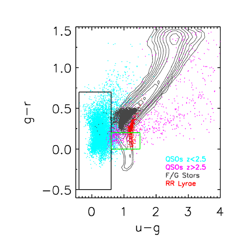
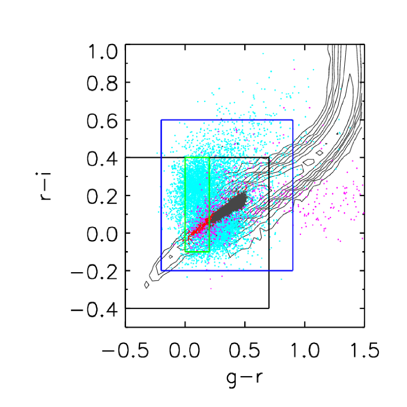
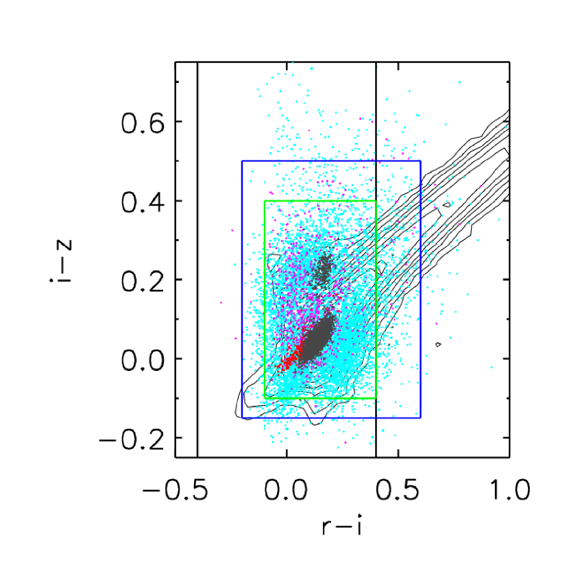
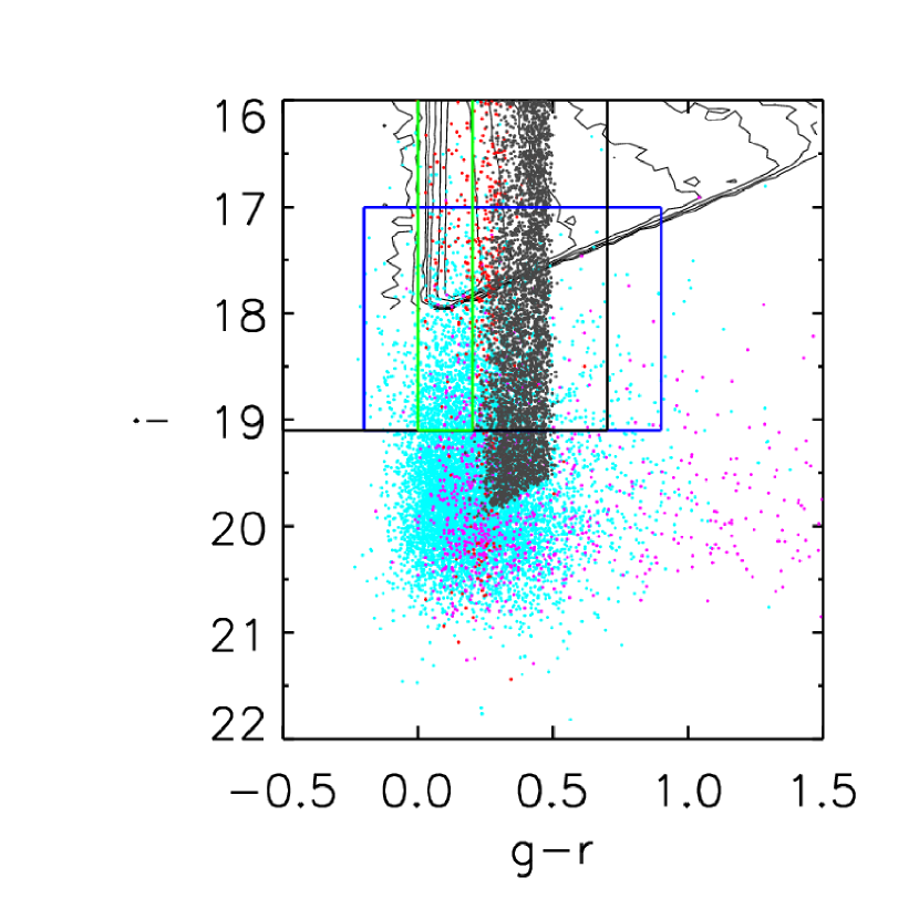
The most common way to generate large samples of optical quasar candidates for follow-up is by specifying a particular region of interest in color space, as was done e.g. in SDSS (Richards et al., 2002a, 2006, 2009). For quasars at the color is crucial in this approach since it enables a photometric separation of the quasar candidates from the stellar locus, reducing the number of contaminating objects to a point where spectroscopic follow-up is feasible. This is illustrated in Figure 1, where we have plotted the median color of 9000 spectroscopically confirmed quasars, as well as an illustrative comparison sample of 5000 F/G and 483 RR Lyrae stars (see Section 3), all drawn from the SDSS Stripe 82 photometric catalog DR7 (Abazajian et al., 2009). The top panels and the bottom left panel of Figure 1 shows the distribution of the samples in the color-color planes of the SDSS color cube. This clearly shows the power of the color (upper left panel) compared to the , and colors in separating the quasars from their contaminants, especially for low redshift quasars (i.e. shown as light blue points). The color magnitude diagram in the lower right panel illustrates that a cut in magnitude will also eliminate contaminants. The contours indicate the stellar locus of Stripe 82 point sources with
For higher redshift objects (, shown as magenta points in Figure 1) the quasars intersect the stellar locus (top left panel). The purity for quasar candidate samples is around 10-50% in the color-selected SDSS quasar target sample (Richards et al., 2006). In general the color selection method is efficient for low and high redshift quasars, but for the intermediate redshift objects contamination becomes a severe problem. We refer to Figures 13 and 14 in Richards et al. (2002a) for a more complete version of Figure 1.
With Pan-STARRS 1 (henceforth PS1) the contamination problem is even more pronounced when using the color selection method only. PS1 has a 5-filter system consisting of SDSS-like , , , bands (albeit with significantly higher red sensitivity) and a filter. The crucial color used in the SDSS color selection method is not available: the contamination of a color-selected PS1 quasar sample will be a problem for as well as for . It is therefore necessary to find a way of separating the majority of quasars from the contaminating stellar locus in order to obtain a pure PS1 quasar sample. The intrinsic variability of the quasars (and their contaminants) is a very promising tool for doing this.
2.2. Source variability: power-law structure functions
The structure function characterizes the variability of quasars (and the other sources) by quantifying the variability amplitude as a function of the time lag between compared observations (Cristiani et al., 1996; Giveon et al., 1999; Eyer, 2002; Vanden Berk et al., 2004; de Vries et al., 2005; Rengstorf et al., 2006). For any object the observables for estimating the structure function are the data pairs, assuming light curve data points, describing the variability as the magnitude difference between two epochs and , corrected for measurement errors, i.e.,
| (1) |
Here is the measured magnitude difference between observation and . The and are the photometric errors on the measurements and is the time difference between the two observations. The quantity is defined like this so that its average, over a large number of data pairs, is an estimator for the intrinsic standard deviation of the source magnitude.
At this point we note that usually refers to the time lag in the quasar rest frame. However, computing this requires a priori knowledge of the quasar redshift, and when selecting objects in imaging-only surveys, we do not know the object redshift. Therefore, we work with time lags in the observed frame. This necessary convention differs from most of the quasar variability literature; we will make some comparisons in Section 4.
In previous analyses, the average has been calculated in time lag bins using data pairs from many quasars, thus “stacking” the variability signal to allow the properties of the quasar population to be probed. Then
| (2) |
where the average, , is taken over all epoch pairs , whose lag falls in the bin . The same approach can be taken in estimating the structure function of classes of objects (e.g. quasars at a given luminosity and redshift bin) if, say, only two epochs are available per object, but large samples exist (e.g. Richards et al. (2006, 2009)); in that case the in Equation 2 becomes and ensemble average. Vanden Berk et al. (2004) and others find that the ensemble average quasar structure function appears to follow an increasing power law with time lag.
On the other hand, for the case where the light curve sampling of each object is high, we can compute the average for an individual object (Eyer, 2002). Binning the data pairs from an object’s -point light curve gives an estimate of defined at each bin center. This approach is computationally efficient, and provides a free-form view of the object’s structure function. However, in the case of relatively sparse sampled data (6 epochs over 3 years in the PS1 survey, see Section 3.7), binning the data pairs to obtain the structure function from Equation 2 to estimate the variability may not be the optimal approach.
In Equation 2, both the noise and the intrinsic photometric variability are assumed (implicitly) to have a Gaussian distribution (Rengstorf et al., 2006). We can then extend this simple model of quasar variability to include a power law increase in variability with time lag. Drawing on the results from Richards et al. (2006) we propose a power-law model for the structure function given by
| (3) |
We can then fit this model to a given set of data, , as follows. We write the likelihood for the power law parameters and as
| (4) |
assuming a set of independent magnitude differences as our data. Here is the likelihood of observing one particular magnitude difference between two light curve points separated by . Following the ensemble analyses referred to above, we assume an underlying Gaussian distribution of values and Gaussian photometric errors:
| (5) |
Here, the effective (observed) variability is
| (6) |
i.e., we propagate the photometric errors and by adding them in quadrature to the variability “error”
This approach can yield posterior probability distributions on the two model parameters, and . The amplitude quantifies the root-mean-square magnitude difference on a 1 year timescale, while is the logarithmic gradient of this mean change in magnitude. We assign uninformative priors for the parameters (uniform in the logarithm of , and uniform in the arctangent of – since represents the slope of a straight line), and then explore the posterior probability distribution for these two power law parameters via a simple Markov chain Monte Carlo (MCMC) code (Metropolis et al., 1953; Hastings, 1970) as described in Appendix A. All we are doing is replacing binned structure function parameters (the values of in each of the bins) with two parameters that define a power law structure function, and then inferring these parameters instead of constructing estimators for them. We will show in Section 4 that using a power law model for the variability actually provides a good fit.
3. SDSS Stripe 82: a Testbed for Variability Studies
Anticipating the results of Section 4, we note that to detect and quantify intrinsic quasar variability will likely require multi-epoch data spanning several years. Before surveys with facilities such as Pan-STARRS and LSST become available, SDSS Stripe 82 (Abazajian et al., 2009) forms an excellent training set and methodological test bed (e.g. Sullivan et al., 2005; Sesar et al., 2007; Bramich et al., 2008; Frieman et al., 2008). In this section we will describe the various Stripe 82 data sets that we have created in order to test and illustrate the prospects of our algorithm.
The SDSS Stripe 82 region (henceforth S82) covers approximately 320 deg2, from right ascension around 290∘ to 60∘ in a wide band on the celestial equator. Over eight observing seasons it has been repeatedly observed in the fall months, resulting in many epochs (typically 60) in each of the 5 SDSS bands. As the PS1 survey will contain fewer epochs, we can “down-sample” the S82 object light curves to simulate observations taken with PS1 (albeit ones at lower angular resolution and depth).
Relative to PS1, S82 does have the advantage of color coverage, and extensive bright object spectroscopy. One can therefore construct quite pure samples of quasars, RR Lyrae and so on, that may serve as ground truth for our variability selection.
In the following subsections we describe these various subsamples in some detail, and provide a brief overview here. We have selected all the spectroscopically confirmed quasars in S82 together with a representative set of (stellar locus) contaminants, which contains non-varying (type F/G stars) as well as varying (RR Lyrae) point sources to illustrate our method and algorithm prospects. These objects’ photometry data are plotted in color space in Figure 1. To investigate the selection of quasars by their colors, we define three color selection boxes and explore the objects returned by each. One of these mimics the more limited color selection possible with PS1: quantifying how the variability information then improves the PS1 quasar selection is one of the main goals of this paper.
In the following subsections, we describe two preparatory steps for turning the 60 epoch S82 data into a testbed for color plus variability based quasar selection in SDSS (S82) and PS1: first, we describe the definition of various sub-sets of candidate objects; then we describe some technical steps “cleaning” the light curves and down-sampling the S82 data to mimic PS1.
3.1. Spectroscopically-confirmed quasars in Stripe 82
Key to designing a quasar variability selection algorithm is an understanding of the variability properties of objects that are indeed spectroscopically confirmed quasars. We have selected all of these (both point sources and extended objects) published in the SDSS DR5 quasar catalog (Schneider et al., 2007) that fall within S82. There are 9157 spectroscopically confirmed DR5 quasars in S82, spanning a redshift range from 0.08 to 5.09. These quasars have with a mean of 19.5. See Schneider et al. (2007) for the corresponding numbers for the whole DR5 quasar catalog.
To get the multi-epoch photometry (light curves) for the 9157 quasars we
performed an SQL neighbor search in the S82 DR7 database,
choosing a search radius of
0.5” to minimize the light curve contamination from
misidentified (spatial) neighbors.
This search on average yielded 60 epochs per object, after
selecting only entries with
good BRIGHT, EDGE, BLENDED, NODEBLEND,
SATUR, PEAKCENTER, NOTCHECKED, INTERP_CENTER and
DEBLEND_NOPEAK flags (of which the first 5 are referred to as fatal and
the rest as non-fatal flags by Richards et al. (2002a) – see their Table 2 or
Stoughton et al. (2002) Table 9 for a description of the flags).
For consistency
we applied these same flag checks on all object samples we drew from the
S82 catalog.
We describe these other samples below.
3.2. Stellar locus “contaminants” in Stripe 82
To get a sample of typical non-variable stellar contaminants we used the SDSS standard star catalog of 1.01 million non-variable point-source objects in S82 published in Ivezic et al. (2007). From that we created a set of F/G-star colored objects, presumably non-varying, by applying a color-magnitude cut on the standard star catalog so that and for all the objects. This is a suitable cut for F/G-stars according to the SEGUE team (Yanny et al., 2009) and makes them potential quasar sample contaminants because of their color (see Figure 1). We took a randomly selected subsample of 5000 objects from this catalog and did a neighbor search in S82 to get multi-epoch observations of these contaminants. We again used a search radius of 0.5” and again made sure that none of the flags listed in Section 3.1 were set.
To be able to test whether our algorithm is able to separate quasars from known variable contaminants, we used the largest available sample of securely identified RR Lyrae within S82 (Sesar et al., 2010), which consists of 483 RR Lyrae.
We will refer to the F/G stars and RR Lyrae catalogs collectively as the “contaminants” in the remainder of the paper.
3.3. UV-excess (UVX) objects
We would also like to test our ability to detect quasars in the absence of spectroscopic data. To this end, we defined three photometrically-selected samples of S82 objects, whose variability properties we will explore.
The first of these is defined by a three-dimensional color box in which the SDSS quasar sample is complete for extinction-corrected magnitudes brighter than 19.1 (Richards et al., 2002a). This color box is given in Table 1, and is shown in black lines in Figure 1. Note that this selection uses the SDSS -band data: we extracted all point sources within S82 that obeyed these “UV excess” (UVX) criteria. This returned a catalog of 2912 UVX point sources.
| -0.4 | 0.6 | |
| -0.5 | 0.7 | |
| -0.4 | 0.4 | |
| 19.1 |
3.4. Non-UV excess (nUVX) objects
As a compliment to the UVX object sample defined above, where the color selection is known to efficiently return quasars at high completeness, a catalog of “non-UVX” (nUVX) objects was created from a region of color space where color selection of quasars is known to have problems. The color box from which we selected these nUVX point sources is given in Table 2, and shown as a green box in Figure 1 (and also Figure 7 of Richards et al., 2002a). In this particular color box, the quasar locus, containing mostly intermediate redshift () quasars, crosses the stellar locus. The color selection therefore has efficiency as low as 10% in this region of color space (Richards et al., 2006). In the nUVX color box we find 3258 objects in S82.
| 0.6 | 1.5 | |
| 0.0 | 0.2 | |
| -0.1 | 0.4 | |
| -0.1 | 0.4 | |
| 19.1 |
3.5. Quasar Candidate Color Selection without -band Data
To simulate approximately the anticipated PS1 survey light curves, we defined a third color box suitable for a first cut of the PS1 catalog. The main purpose of this selection (where no -band information is used) is to excise the quasar locus as it threads through the 3-dimensional color space. However, part of the stellar locus also lies in this box. We restrict ourselves to right ascensions between 0 and 20 degrees (enclosing a sixth of the S82 area, 50 deg2) in order to return a manageable catalog of 12,714 objects. The box is indicated by the blue solid lines in Figure 1 and is defined in Table 3. The magnitude cut of 19.1 is chosen to allow straightforward comparison with the UVX and nUVX boxes.
| -0.2 | 0.9 | |
| -0.2 | 0.6 | |
| -0.15 | 0.5 | |
| 17 | 19.1 |
3.6. Eliminating light curve “outliers” in Stripe 82
Plotting the complete S82 multi-epoch photometry output for the various objects revealed some outlying points that were several magnitudes fainter than adjacent flux points (see Figure 2); only some of these outliers were found to be caused by image defects. However, we assume that such a significant decrease in magnitude in a single observation must be non-physical. We therefore removed the outliers (irrespective of their origin) by running a median filter on the photometric measurements. Measurements with a residual between the medianized light curve and the photometric data larger than 0.25 magnitudes were removed. In Figure 2 we show the , and -band multi-epoch photometric measurements (open symbols indicating the removed measurements) with the corresponding medianized light curves over-plotted for quasar SDSS J203817.37+003029.8. The bottom panel shows the residuals, with the limit of 0.25 magnitudes indicated by the dashed lines. As is the case here, in general, only a small fraction of the epochs is removed.
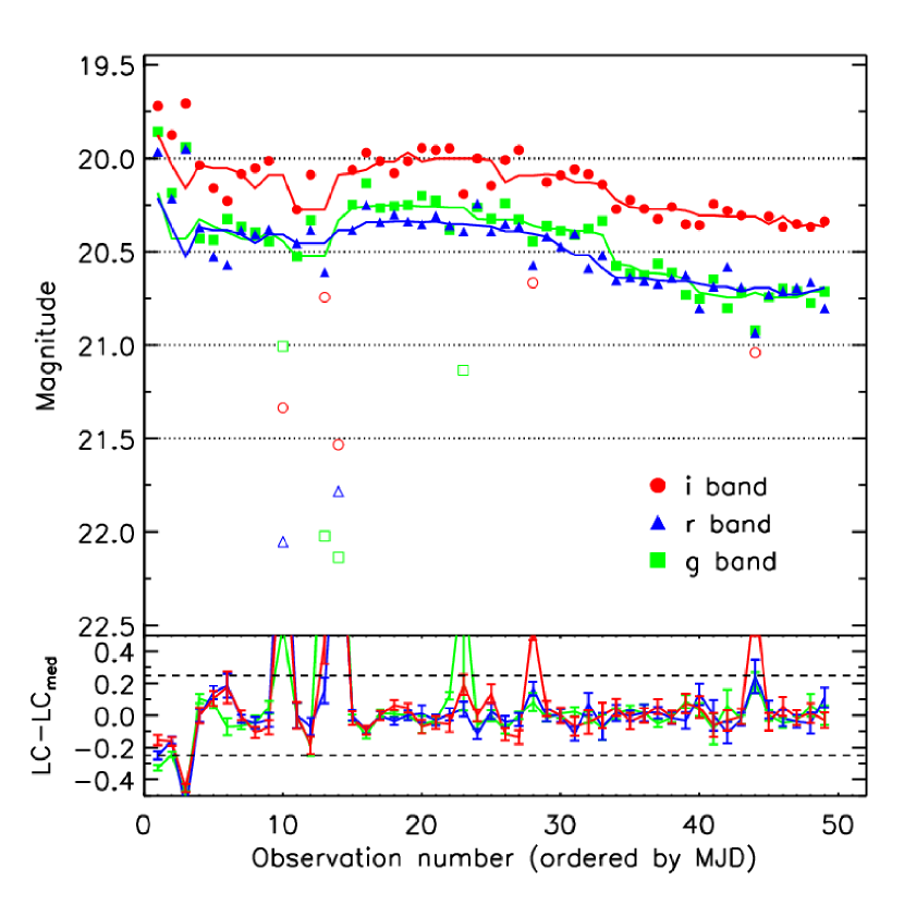
It is these cleaned multi-epoch measurements, where the outlying observations have been removed (i.e. the filled symbols in Figure 2), we use in the determination and exploration of the objects’ variability.
3.7. Down-sampling S82 light curves to the PS1 cadence
In order to explore quasar selection in the context of the PS1 survey, we down-sampled the S82 data to mimic the planned PS1 observations (Chambers & Dennau, 2008, shown schematically in Table 4). We assumed 3 observing seasons for PS1, with a duration of 155 days (covering all filters) each. Only S82 objects with more than 7 epochs in each (SDSS) season were passed to the actual down-sampling routine: 1% of the quasars, of the F/G stars and 20% of the RR Lyrae did not satisfy this criteria.
We down-sampled the S82 light curve data by matching each season of observations for the , , and -band with the (approximately) correct time intervals between consecutive observations in each band. No color information went into the down-sampling. After identifying 6 suitable S82 epochs in each band we removed all other observations, providing a set of mock PS1 data.
| Date (days) | -60 | . | . | . | . | . | -30 | . | . | . | . | . | 0 | 5 | 10 | . | . | . | 30 | 35 | 40 | . | . | . | 60 | . | . | . | . | . | 90 |
|---|---|---|---|---|---|---|---|---|---|---|---|---|---|---|---|---|---|---|---|---|---|---|---|---|---|---|---|---|---|---|---|
| Band | . | . | . | . | . | . | . | . | . | . | . | . | . | . | . | . | . | . | . | . | . | ||||||||||
| Moon | F | . | . | N | . | . | F | . | . | N | . | . | F | . | . | N | . | . | F | . | . | N | . | . | F | . | . | N | . | . | F |
Notes: Date is calculated with respect to the first -band measurements. Band shows the band observed. Moon indicates whether the moon is full (F) or new (N). The columns are spaced by five days.
4. Power-Law Structure Functions for Sources in Stripe 82
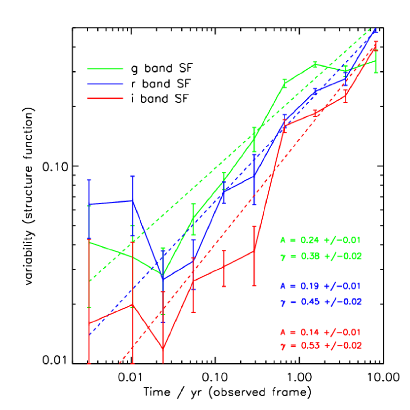
In Figure 3 we show the binned structure functions (Equation 2) from the , and -band light curves of quasar SDSS J203817.37+003029.8 (Figure 2). Calculating binned structure functions for individual S82 objects is a simple way of quantifying the variability of each object if there is a large number of epochs available. However, Figure 3 suggests that we might indeed be justified in further compressing the structure function into a two parameters power-law fit, as proposed in Section 2.2.
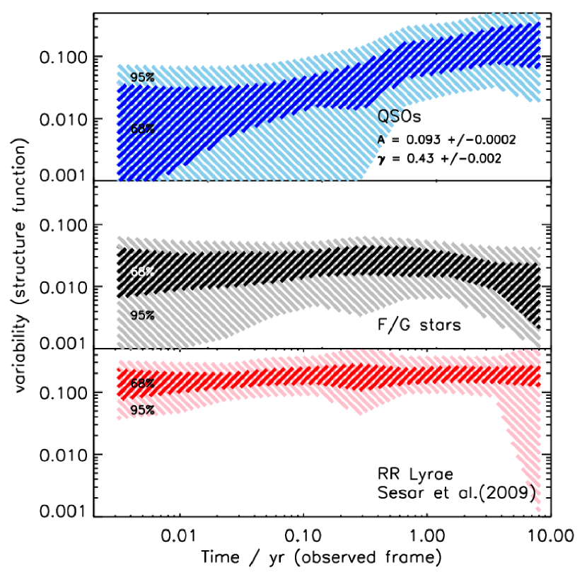
Before doing so, we explore wether this power law behavior is present in an average sense. In Figure 4 we show the median sample structure function, created by median-combining all the individual binned structure functions calculated with Equation 2 separately for the well sampled S82 quasars (Section 3.1), F/G-stars (Section 3.2) and RR Lyrae (Section 3.2 and Sesar et al., 2010). The shaded regions in Figure 4 around the medians enclose 68% and 95% of the individual structure functions. Figure 4 shows that the quasar sample median of the binned structure function closely resembles a power law with and , in agreement with findings elsewhere in the literature (Vanden Berk et al., 2004; Rengstorf et al., 2006; Wilhite et al., 2008; Bauer et al., 2009). In particular, a value of the slope of the sample median structure function of agrees well with most of the literature (see e.g. Table 4 in Bauer et al. (2009) for a brief overview). Rough estimates of the 1-year observed frame power law amplitudes in the literature give amplitudes between 0.10 and 0.14 (depending on the assumed mean redshift of the samples), in good agreement with our estimate for of 0.093 mag.
Figure 4 also shows that the sample structure functions of contaminants are also well described by power laws, but with small values of (i.e. they show no long-term growth in their variability). Note that the F/G-stars, chosen to be non-variable, have a variability amplitude of 0.04 mag. The RR Lyrae variability, when sparsely and randomly sampled in S82, looks like white noise () with an amplitude 0.2 mag. Thus, the use of a power-law model of the form given in Equation 3 would seem to be a fairly good assumption, and different types of objects may differ both in amplitude and in slope of their structure function.
In Figure 3 the power law fits to the three (binned) structure functions are shown as dashed lines. The and with their estimated errors are given in the lower right corner of the plot.
5. Results
Having defined different sub-samples of sources, and having shown that we can sensibly quantify their light curve characteristics by a power-law structure function model, we now proceed to characterize each of these sources by their best-fit parameters and .
As opposed to the earlier SDSS analysis (Richards et al., 2002a, 2006, 2009) the improved time sampling of the S82 (and even PS1) surveys, enables us to investigate the distributions of the and parameters for the individual sources, not only for ensembles.
5.1. The A- Distribution
Figure 5 shows the distribution of the variability characteristics, quantified by the best-fit and for all the spectroscopically confirmed quasars, and for the “contaminant” F/G stars and RR Lyrae, as described in Section 3, based on their -band S82 light curves. The histograms along the axes of the two dimensional scatter plot show the projected parameter distribution of the quasars and of the contaminants. Visual inspection of Figure 5 alone shows how well the spectroscopically confirmed quasars separate from the (stellar locus) contaminants in this space, demonstrating that the power-law structure function fit from a single band is an efficient classifier for data of this quality (60 epochs).
The analogous - distributions for the much sparser PS1-like sampling of the -band measurements (Section 3.7) are shown in Figure 6: these parameter estimates are based on only 6 epochs of photometry over 3 years, rather than the in the full S82 survey. The separation of the quasars and the contaminants is less clean with the PS1 sampling, but one nevertheless clearly sees a quasar-dominated region with rather low contamination. Plots analogous to the ones shown in Figures 5 and 6, but for the , and -band measurements, show that on average decreases by 30-50% going from to band, whereas is unchanged with varying wavelength. Thus, the separation of the quasars from the contaminants via their values appears to work comparably well in all 4 bands (with somewhat more scatter in the -band). In agreement with Kozlowski et al. (2010), no clear difference in the ratio of the amplitudes at different wavelengths between RR Lyrae and quasars is detected.
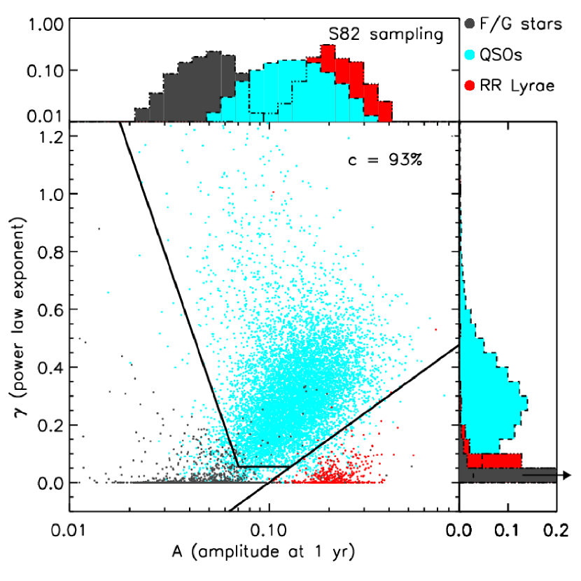
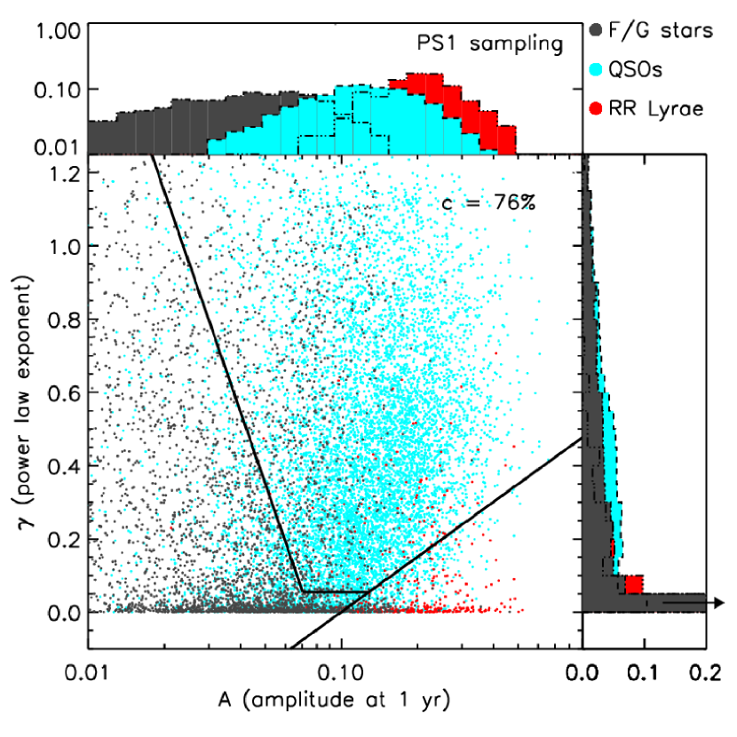
Since most F/G-stars should not vary, but RR Lyrae do, they should have different distributions. This is seen in Figure 5 and 6: RR Lyrae have magnitude amplitudes above 0.1 (e.g. Soszynski et al., 2003; Sesar et al., 2010), while the F/G-stars have characteristic values of . It is therefore clear that our approach can also separate RR Lyrae from stellar (non-varying) contaminants without doing a full fit of a periodic light curve.
5.2. Completeness and Purity
To move beyond a merely qualitative assessment of the separability of the quasars from contaminants we now estimate the achievable completeness and purity of the resulting sample. Purity is the more difficult quantity to estimate as it requires appropriate abundances for the contaminants. We do not have these for the training set parent quasar, F/G star and RR Lyrae samples, where the ratio of quasars to contaminants is 2:1, instead of a more realistic 1:25, and therefore can only estimate completeness when working with these samples. However, by design the UVX, nUVX and selection boxes (Sections 3.3–3.5 and 5.2.1–5.2.3) give parent samples with the correct quasar-contaminants ratio: we use these to explore the purity of our quasar selection algorithm.
For the present we divide the - plane by simple cuts that define a quasar selection box, and then quantify its performance. Specifically, our fiducial quasar selection region is bounded by the following three straight lines:
| (7) | |||||
| (8) | |||||
| (9) |
This can be thought of as a way of providing lower limits on the available completeness and purity, that a more sophisticated selection procedure would improve upon. One could of course tweak the cuts in Equations 7–9 to explore the trade-off between purity and completeness, which we have only done here “by eye.”
Applying these cuts to the data leads to the completeness given in Table 5 for the “QSO+contam” catalog. The completeness is calculated as the fraction of spectroscopically confirmed quasars in the sample that fall within the cuts. In our simple illustrative setup we have a completeness of 93% for the quasars in the case where the time sampling is equal to Stripe 82 (60 epochs). In the case of a PS1-like time sampling the completeness drops to 76%.
| Parent Catalog | Sampling | p | Quasar Reference Catalog | |||
|---|---|---|---|---|---|---|
| QSO+contam. | S82 | 93% | 1% | - | - | SDSS |
| QSO+contam. | PS1 | 76% | 1% | - | - | SDSS |
| UVX | S82 | 90% | 3% | 95% | 3% | SDSS+2SLAQ |
| UVX | PS1 | 73% | 2% | 92% | 3% | SDSS+2SLAQ |
| nUVX | S82 | 90% | 15% | 96% | 16% | Visual |
| nUVX | PS1 | 65% | 12% | 32% | 5% | Visual |
| box | S82 | 92% | 6% | 92% | 6% | Visual & SDSS+2SLAQ |
| box | PS1 | 75% | 6% | 30% | 2% | Visual & SDSS+2SLAQ |
Of the RR Lyrae 97% and 83% (for the S82 and PS1 sampling respectively) fall in the high- low- corner below the line given by Equation 7. In this region 0.5% of the 5000 F/G-stars lie, illustrating quite a clean separation between RR Lyrae and non-varying stellar contaminants.
Besides calculating the overall completeness, we also split our data into redshift bins. The completeness of the quasars is rather constant as a function of redshift, with a minor loss of about 5-10% for redshifts above 4. Since our training set only contains 52 quasars at , we were not able to investigate this decreased completeness further.
In the next three subsections we proceed to explore the - distributions for the samples of objects that were selected only on the basis of their colors (Table 1, 2 and 3). For those samples, we estimate the completeness (as above) and also the purity, defined as the fraction of known quasars compared to the total number of objects inside the - selection regions.
5.2.1 Quasars in the UVX catalog
For the UVX object sample (Section 3.3) there is enough spectroscopy in S82 to define a spectroscopically confirmed quasar subsample, a reference catalog of quasars which is complete in S82. By combining the spectroscopically confirmed quasars in S82 (Section 3.1), with the objects from the 2SLAQ (2-degree field SDSS luminous red galaxies and QSO) survey(Croom et al., 2009a), our final quasar reference catalog contains 11216 individual quasars (9157 from SDSS and 2059 from 2SLAQ). We only selected objects flagged as “QSO” in the publicly available 2SLAQ data.111http://www.2slaq.info/
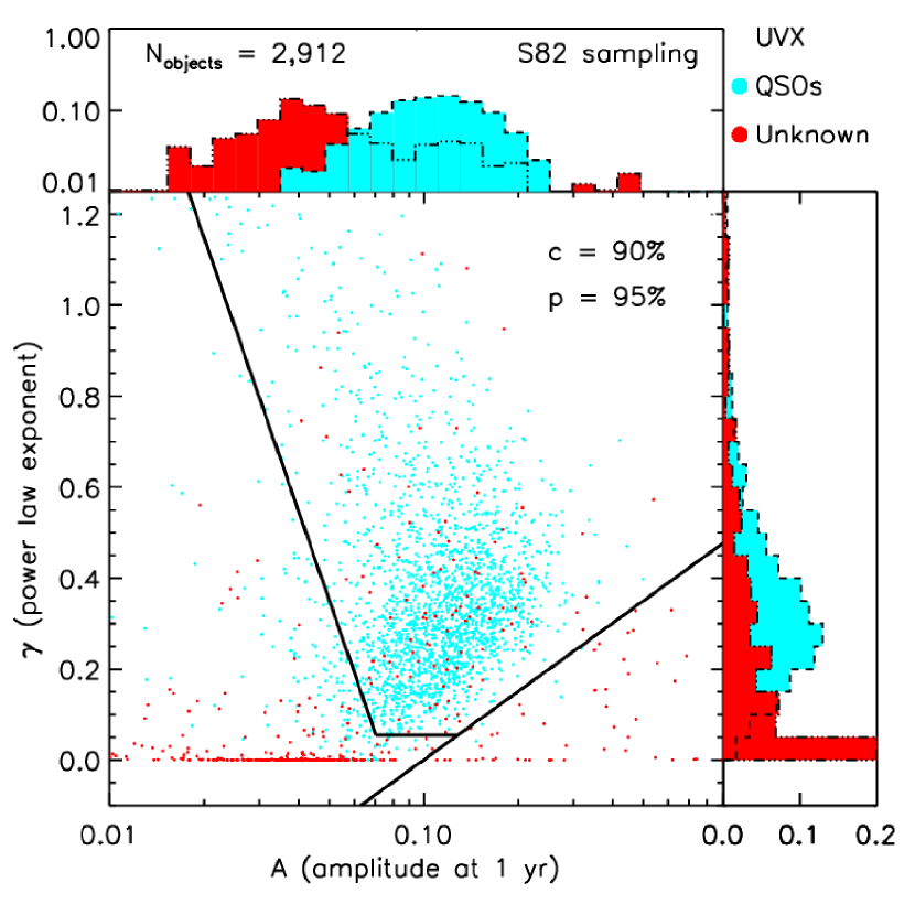
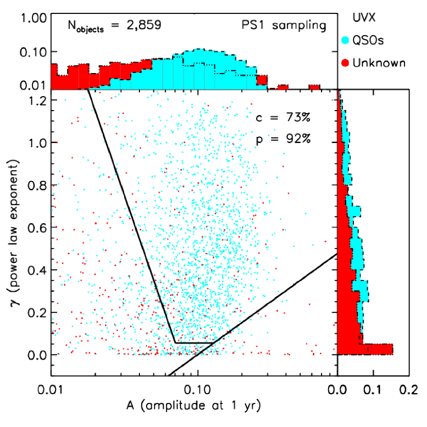
Matching this quasar reference catalog with the catalog of UVX S82 point sources returned 2140 quasars out of the 2912 objects in the UVX catalog. Thus, 73% percent of the point sources in the UVX color box are known quasars. It is not surprising that the fraction is so large, since we used the powerful color in the definition of the color box. This simply re-affirms that the UVX box is a region of color space where the quasars are in the majority, as they are well separated from the stellar locus by the color; it is exactly this separation to which we are trying to find an alternative.
We estimated and for the entire UVX catalog, using both the full (S82) sampling and the sparser PS1-like version of it. The result is shown in the top row of the - plots in Figure 7. Applying our simple variability selection cuts (Equations 7–9) returned 2033 and 1734 quasar candidates for the S82 and PS1 sampling, respectively. Matching these objects with the 2140 know SDSS+2SLAQ quasars in the UVX catalog returned 1935 and 1573 matches. Thus we are able to detect the UVX quasars with a completeness of 90% and a purity of 95% (1935 matches/2033 candidates) when using the S82 time sampled data. For the PS1-like sampling of the data we get a completeness of 73% and a purity of 92% (Table 5).
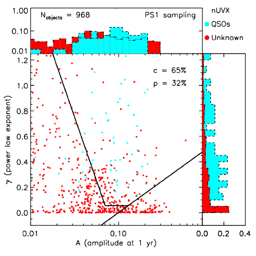
5.2.2 Quasars in the nUVX catalog
The catalog of the UVX point sources was deliberately chosen from a region of color space where the color selection already does a superb job finding quasars, as confirmed by the complete SDSS and 2SLAQ quasar catalog and the completeness and purity of our - approach. However, one might argue that in this case (of UVX quasars) a light curve analysis adds little. To explore the - approach further we applied it to the non-UV excess objects described in Section 3.4.
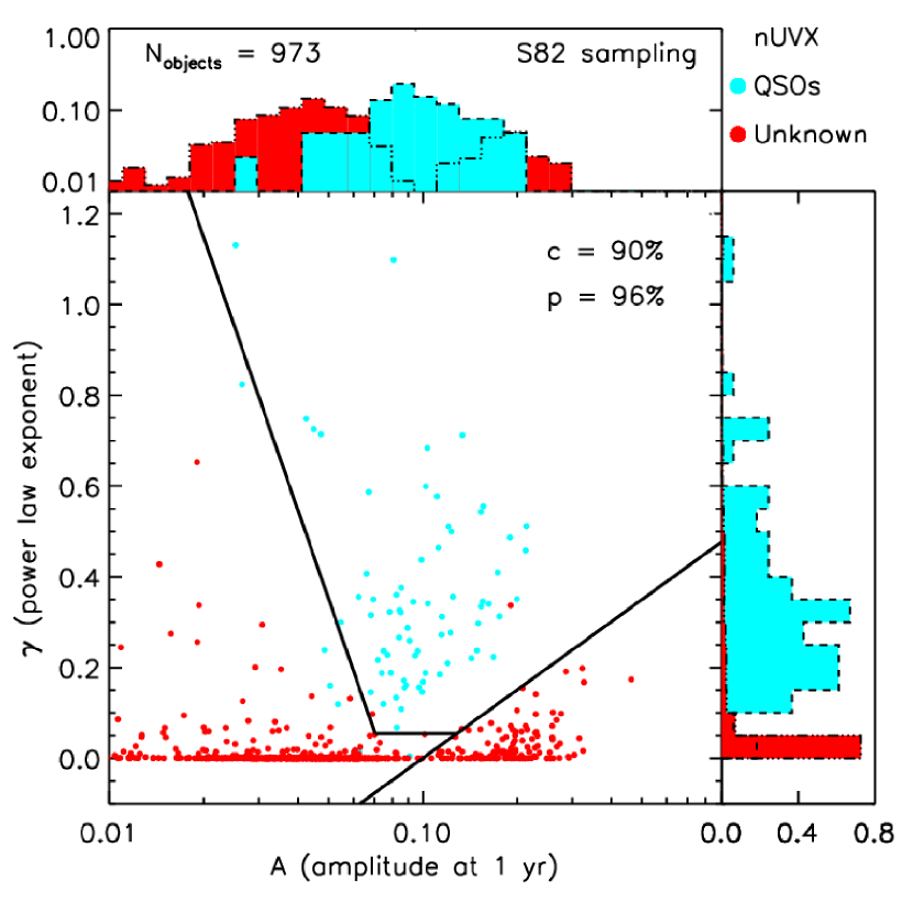
In the nUVX color box (Table 2) there is no simple way to quantify the completeness of the parent sample of color-selected objects, since we do not know how many quasars were missed in this region of color space during the SDSS survey. To try to quantify this, we extracted the spectra from the 973 objects in this catalog that were targeted for SDSS spectroscopy. By visually inspecting these spectra we were able to compile a catalog of 77 quasars among the S82 nUVX objects. (Of these 77, 6 quasars are not in the SDSS+2SLAQ catalog). This means that if the SDSS fibers had been allocated to nUVX objects randomly, then the purity of the nUVX quasar sample would be %. However, in practice the fibers were placed according to a Bayesian ranking that made fuller use of the color information, so that this 8% is likely an upper limit on the purity of the nUVX quasar sample. (The fraction of quasars hidden in the un-targeted nUVX objects is likely lower than the fraction of quasars found in the nUVX objects with spectra.)
Applying our - analysis and our variability selection criteria to the spectroscopic sub-catalog of 973 nUVX objects returned 72 (178) quasar candidates for the S82 (PS1-like) time sampling. The nUVX objects’ variability parameters are plotted in the bottom row of Figure 7. Estimating the completeness and purity in the S82 sampling case, assuming that the 973 objects with spectra are a random subset of all the nUVX objects, gives that we are 90% complete and 96% pure (Table 5). By the same argument as above, the purity is an upper limit on the overall purity of the nUVX quasar sample whereas the completeness is exact. The purity and the completeness stand on their own in quantifying our ability to recover the spectroscopically confirmed quasars. Thus, the addition of the variability information enhances the purity to 96% instead of 8%, as is the case for the pure color selected sample. In the case of the sparser PS1-like sampling we still have a completeness of 65%, and a purity of 32%. This clearly demonstrates that a variability-based approach is very efficient at selecting nUVX quasars when the data is well sampled in time. Even with the sparse PS1 sampling, the purity increases by a factor of four when variability information is used.
The plot of the S82-sampled nUVX objects (lower left corner of Figure 7) shows a clear bimodality of the parameter distribution of the unknown (red) objects. As seen with the object training set, this bimodality is a probable separation between the non-varying contaminants and the varying (possible RR Lyrae) contaminants. Thus the nUVX objects have been separated into quasar candidates (high ; intermediate ), RR Lyrae candidates (low ; high ) and non-varying stars (low ; low ).
5.2.3 Quasars in the Color Box
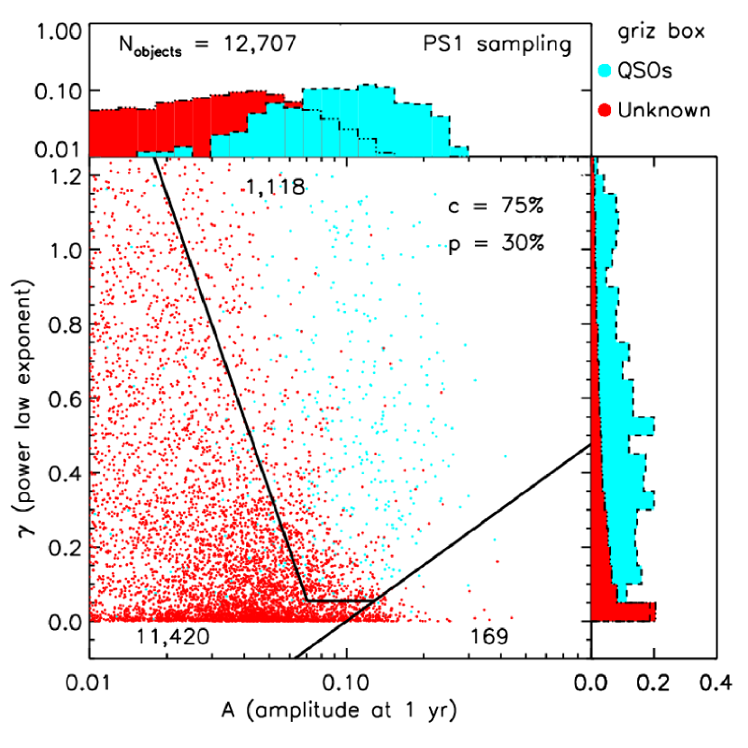
To simulate quasar candidate selection without -band photometry, we applied our variability analysis to the objects lying in a fairly large multi-color region in space, the so-called box defined in Section 3.5. This color box fully contains an important part of the stellar locus. Estimating the completeness and purity of our algorithm for the box is difficult, as no clear estimates of the abundance of quasars exist for such a color cut. We therefore checked the quasar candidates against a catalog of the SDSS+2SLAQ quasars, plus the 6 extra quasars found via the visual inspection of the nUVX spectra. This may fall considerably short of a complete sample of quasars, but at the moment it is the best we can do; the purities calculated in this section are therefore lower limits. Matching this quasar reference catalog to the 12,714 objects in the box we found 443 known quasars. Estimating - for all these sources, returned 442 (1,118) variability-based quasar candidates, when considering the S82 (PS1) sampling and when applying the - cuts of Equations 7–9. Of these candidates 407 (333) were found to be known quasars. Thus, for the broad color pre-selection, variability selection achieves 92%(75%) completeness and a purity of 92%(30%) for the S82 (PS1) sampled data, respectively. The and distributions for the box selected objects are shown in the top panel of Figures 8 (S82 sampling) and 9 (PS1 sampling).
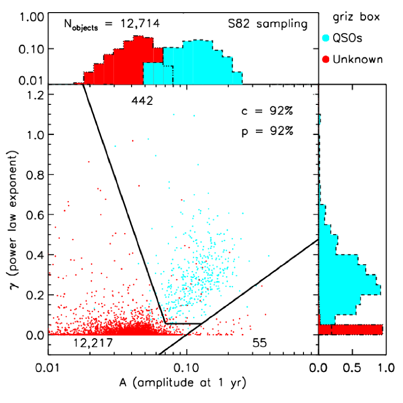
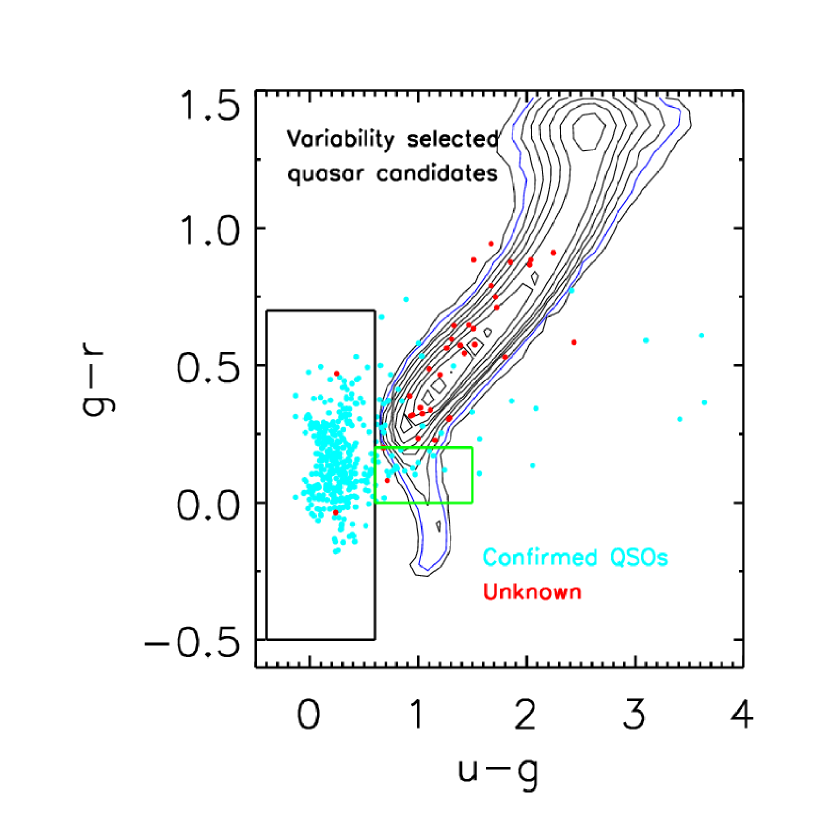
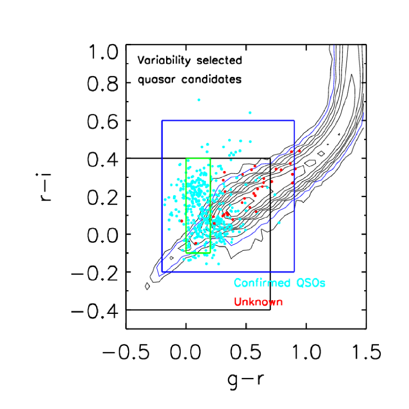
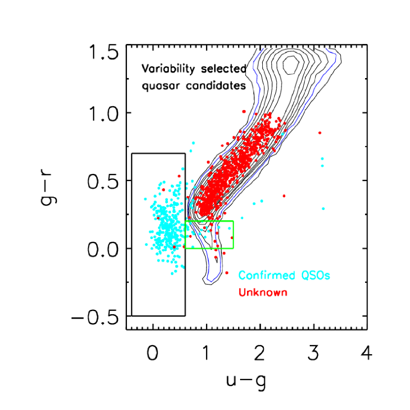
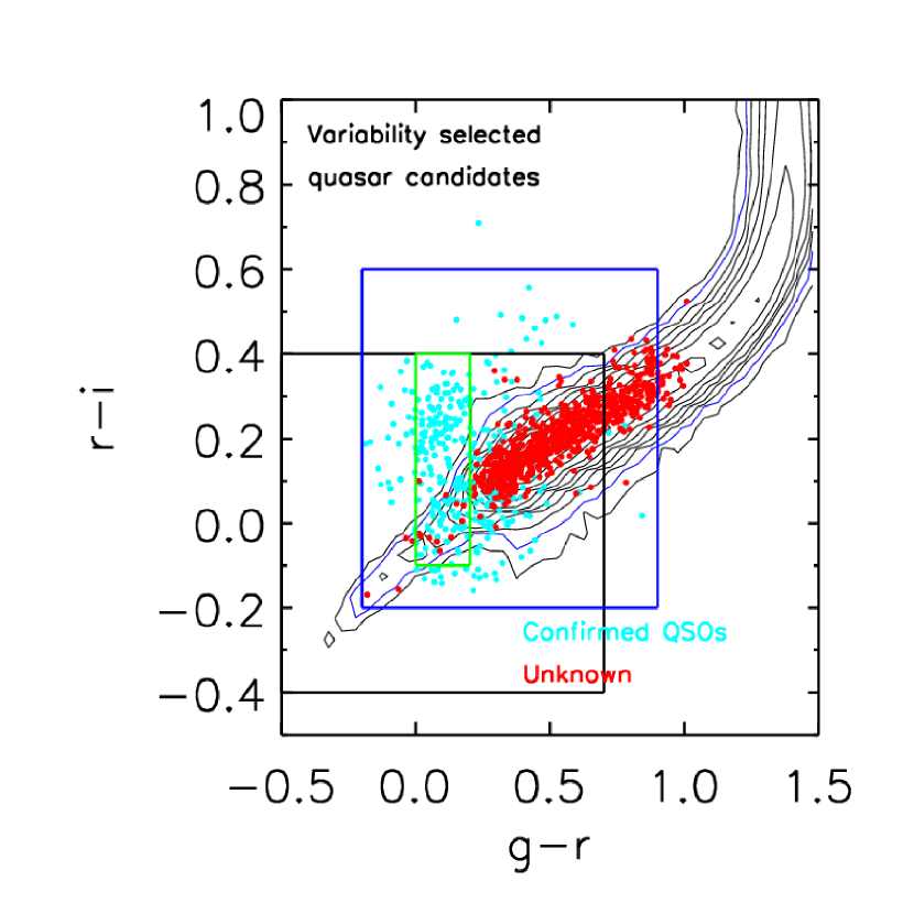
In the bottom panel of Figure 8 and 9 we have projected our variability selected quasar candidates back into and color space, in order to understand the color distributions of variability selected quasar candidates. The figures show that 86% and 98% of the not spectroscopically confirmed candidates fall on the stellar locus, defined as the (blue) contour level containing 95% of the stellar locus objects in S82. This suggests that many, if not most, of these unconfirmed quasar candidates are stars scattered into our variability-selection region. However, there are some possible quasars among the unknowns judging from their colors. For instance, a few of the unknown objects (6% and 1% in the S82 and PS1 sampled case respectively) fall in the UVX selection box. This illustrates that our purity estimates are lower limits but close to the likely truth. It also shows that the quasar color selection in SDSS (Richards et al., 2002a, 2006, 2009) has done an excellent job, implying that of the quasars with are “hiding” in the stellar locus and have been missed by the SDSS selection.
When defining the box in Section 3.5 we included the stellar locus to achieve as high a completeness as possible and to illustrate the prospects of our approach. However, removing objects falling within the stellar locus, could greatly enhance the purity at a modest reduction of the completeness. Thus, selecting quasar candidates without -band information can be put into four scenarios:
-
1)
A “naive” box () including the stellar locus and not considering variability information will have a quasar selection completeness above 90%, but a purity of only 4%.
- 2)
-
3)
Combining a color selection including the stellar locus, but considering variability information (illustrated in Figures 8 and 9) leads to a completeness of 92%(75%) and a purity of 92%(30%) for the S82 (PS1) sampled data, respectively. This means that PS1 can provide a 75% complete quasar sample, if 30% purity were acceptable.
-
4)
Finally, removing the stellar locus from the selection box and combining this with variability information lowers the completeness to 54%(44%), but returns a purity of 97%(92%) with S82 (PS1) time-sampled data. PS1 can provide a high purity quasar sample that is 50% complete.
This illustrates how a variability selection cut greatly improves the candidate sample as compared to quasar candidate selection based on colors alone when -band information is not available. Keeping in mind that the purities calculated here are lower limits, these results suggests that the variability selection of quasar candidates in PS1 or other multi-epoch surveys will produce high quality, extensive samples.
6. Discussion
In this paper we have explored the selection of quasars by their variability in lieu of their UV excess in the context of the PS1 survey as a test case for various upcoming multi-epoch surveys. Given its extensive, multi-year time sampling, SDSS Stripe 82 is an excellent test bed, that allows us to address variability selection of quasars (and other sources) in general. Besides PS1 and SDSS, LSST (Ivezic et al., 2008; Abell et al., 2009) and Gaia (Jordi et al., 2006) will be able to employ variability selection similar to that which we have presented.
For any source, we have characterized its variability by a simple power law model for its light curve structure function, which is similar to (but not the same as) MacLeod et al (2008); Sumi et al. (2005); Eyer (2002); Cristiani et al. (1996). For each object the amplitude is the typical variability within 1 year, and the exponent describes how the expectation value for the magnitude differences changes with the time between measurements. Applying this simple variability characterization to spectroscopically confirmed quasars, to presumably non-variable sources (F/G stars) and to known RR Lyrae, we have found that the - space separates these source classes nicely. Quasars have and ; RR Lyrae have and , as the rapid periodic variations in their light curves appear as “white noise” with no secular trend when coarsely sampled on year-long time scales; finally, non-variable sources have . The variability properties for quasars derived here for individual objects with 60-epoch light curves, are consistent with those derived by for instance Vanden Berk et al. (2004) and Bauer et al. (2009) using ensemble averaging. The results allowed the definition of a simple variability-based quasar selection in multi-epoch data, using cuts in the - plane. As we summarize quantitatively below, this variability selection works very well when considering 60-epoch light curves in S82, and still works quite well for the sparser sampling expected for PS1.
The presented algorithm for variability selection is simple enough that it can be applied to large samples. Our IDL code (not optimized for speed) running on two dual-core CPUs takes 2 hours to characterize the 12,000 objects of the color box with the PS1 sampling.
The extensive spectroscopy of quasars in S82 has enabled stringent completeness and purity estimates for variability selection, at least for UVX quasars. Our analysis has shown that variability-based quasar selection with only 6 epochs over 3 years (as for PS1) is effective, producing either complete or pure samples. However, something more like the 60 epochs of S82 is needed to produce variability-selected quasar samples that are both complete and pure (with only weak color pre-selection).
Therefore, it is paramount to eventually combine the variability information in different filters, in order to boost the number of epochs in PS1. We can attempt to do this by predicting time-offset synthetic -band magnitudes from the , , and bands which could reduce the scatter in the - plane, and so enhance the completeness and the purity of the PS1 sampled catalogs. We leave this important extension of our method to further work.
Considerably further in the future, LSST (Ivezic et al., 2008; Abell et al., 2009) will start operating and is planned to ultimately have 200 epochs spread over 10 years. This makes LSST optimal for creating complete and pure variability selected quasar samples. Considering a UVX box like the one used here, a quasar candidate variability selection with the LSST cadence and a 10 year baseline would definitely push both the completeness and purity above the (lower) S82 limits of 90% and 95% shown in the top left plot of Figure 7 and in Table 5. Such samples are expected to be obtainable at least down to LSST’s 10 limiting magnitude of around 23.3 Oguri & Marshall (2010), or even down to 5 () with the 200 epoch variability selection. If we further consider the fact that LSST will have a -band, a LSST color-variability quasar selection will presumably be able to create (UVX) quasar catalogs almost as pure and complete as spectroscopic samples. Hence, LSST will be superior to PS1 in the 20,000 deg2 LSST will observe. However, until LSST happens, PS1 is excellent for improving and further developing variability selection of quasars, and it will provide the first large variability (and -color) selected quasar samples. The LSST (and PS1) quasar catalogs will with estimated sizes of 100 quasars per square degree, or even more, continue the wild growth of quasar catalog sizes seen the last 40-50 years (Richards et al., 2009), and thereby stress that we are on the verge of an era where confirming the quasar nature of all objects in the catalogs by spectroscopic follow-up will be unfeasible. This makes the purity of the photometric samples crucial for doing statistical analyses of the quasars. As demonstrated variability provides purities above 90% for well sampled data at all redshifts and not only for UVX object and will therefore be an important step in achieving very pure photometric quasar catalogs in the future.
7. Conclusions
We have presented a simple, parameterized variability characterization for sources with many epoch photometry. We do this by fitting a power-law model for the structure function of each source’s light curve; the model is specified by an amplitude A and a power-law index .
We have applied this approach to understanding variability-selection of quasars in multi-epoch, multi-color surveys, either augmenting or supplanting the more common color-selection. Specifically, we have analyzed data in SDSS Stripe 82 (S82) both to understand variability selection per se and as a testbed for ongoing and upcoming surveys, such as PS1 and LSST. To predict PS1’s ability to identify quasars, we have down-sampled S82 data to a set of 6 epochs, resembling the expected single-band time sampling in the PS1 3 survey.
For all sources in various sub-samples we calculated the parameters and , and found that for sufficiently many epochs over a multi-year interval, quasars separate well in the - parameter plane from non-variable sources and e.g. RR Lyrae. Quasar variability as typically characterized by and , consistent with earlier ensemble analyses.
Drawing on the nearly complete spectral identification of quasars with in S82, we have explored both the completeness and the purity of single-band, variability-selected quasar samples with both S82 and PS1 time-sampling, and with or without the benefit of -band photometry (which PS1 will not have).
Specifically, we found the following:
-
•
Among the complete, spectroscopically confirmed sample of UV-excess quasars in S82, we can identify 90% of them on the basis of 60 -band epochs over 5 years. This variability selected sample only has a 5% contamination from other objects.
-
•
Repeating the same exercise but with the 10-times sparser PS1 sampling, reduces the completeness to 73% but with still high purity (top right of Figure 7).
-
•
In the redshift range , where quasars overlap with the stellar locus in color-color space, variability can find 90% (65%) of all spectroscopically confirmed quasars for S82 (PS1) sampling. This is a factor of 5-10 more complete than existing color-selection in this particular regime (bottom panel of Figure 7).
-
•
To understand our ability to select quasars through their variability when no -band data are available, we selected all sources in a broad griz color box, known to contain almost all spectroscopically confirmed quasars. In this color box, stars and other contaminants outnumber quasars by a factor of 30 for . Nonetheless, variability selection encompasses 92% (75%) of known quasars for S82 (PS1) sampling. For S82 sampling (Figure 8) the purity of this sample is still very high (92%), but it is rather lower with PS1-like sampling (Figure 9), 30%.
-
•
If in the case of PS1 (6 epochs, no -band) a more pure quasar sample is desired, this can be done by omitting the stellar locus in the box and then looking at the variability of the remaining sources. This yields a completeness of only 44%, but with a purity of 92%.
-
•
The high purity of the variability selected quasar sample in the griz box (with S82 sampling) confirms that the fraction of overlooked quasars in S82 must be small (); this inference is predicted on the assumption that the quasars “buried” in the stellar locus have a variability behavior similar to the others.
- •
As mentioned in the introduction, new and larger quasar samples have many and varied interesting applications. One of these is the possibility of finding lensed quasars. In this work we have only focused on point source selection, with the purpose of finding quasar candidates. Such an approach would be directly applicable to a search for wide separation lenses, where (by definition) the multiple images are well-resolved. Another very interesting use of variability selection, again with quasar lens finding in mind, is to look at spatially extended objects rather than point sources. Applying the algorithm to a set of extended, yet quasar-colored, objects will return a list of small separation quasar lens candidates. We have initiated such a search in Stripe 82 with promising preliminary results, which we will present in a forthcoming paper. This search is a pilot for the PS1 lensed quasar search, which will be able to be started after about a year of survey imaging has been built up. We expect to find as many as 2000 lenses in this database (Oguri & Marshall, 2010). Our analysis illustrates that combining color-selection of quasars with variability selection is a powerful approach to take.
Acknowledgments
We thank Gordon Richards, Xiao-hui Fan and David Hogg for useful discussions, and Branimir Sesar for assistance with the RR Lyrae sample. KBS is funded by and would like to thank the Marie Curie Initial Training Network ELIXIR, which is funded by the Seventh Framework Programme (FP7) of the European Commission. PJM was supported in part by research fellowships from the TABASGO and Kavli foundations, and by the US Department of Energy under contract number DE-AC02-76SF00515.
Funding for the SDSS and SDSS-II has been provided by the Alfred P. Sloan
Foundation, the Participating Institutions, the National Science Foundation,
the U.S. Department of Energy, the National Aeronautics and Space
Administration, the Japanese Monbukagakusho, the Max Planck Society, and the
Higher Education Funding Council for England. The SDSS Web Site is
http://www.sdss.org/.
The SDSS is managed by the Astrophysical Research Consortium for the Participating Institutions. The Participating Institutions are the American Museum of Natural History, Astrophysical Institute Potsdam, University of Basel, University of Cambridge, Case Western Reserve University, University of Chicago, Drexel University, Fermilab, the Institute for Advanced Study, the Japan Participation Group, Johns Hopkins University, the Joint Institute for Nuclear Astrophysics, the Kavli Institute for Particle Astrophysics and Cosmology, the Korean Scientist Group, the Chinese Academy of Sciences (LAMOST), Los Alamos National Laboratory, the Max-Planck-Institute for Astronomy (MPIA), the Max-Planck-Institute for Astrophysics (MPA), New Mexico State University, Ohio State University, University of Pittsburgh, University of Portsmouth, Princeton University, the United States Naval Observatory, and the University of Washington.
Appendix A Individual structure function parameter inference by MCMC
We use a simple Markov chain Monte Carlo (MCMC) approach (e.g. Metropolis et al., 1953; Hastings, 1970; Press et al., 1992; Hansen, 2003) to infer the parameters and (Equation 3) and their confidence regions. Our MCMC procedure takes as input a catalog of magnitudes, photometric errors and observed frame MJDs, converted to pairs of observations (Equation 1). We then initialize it as follows:
-
•
Pick a starting point for and : we chose 0.1 for both
-
•
Define an initial Gaussian proposal distribution (PD)
-
•
Set an initial temperature for the chain
The PD width sets the mobility of the Markov chain. Based on several tests we set the initial PD width to 0.05 in both the and directions. During a “burn-in” period at the start of sampling, we draw samples from a modified posterior PDF for the parameters, given by the product of the prior PDF, and the likelihood raised to the power of . This parameter is an inverse temperature; we start from . The parameter is then increased geometrically to unity as 500 samples are drawn, at which point burn-in is declared over, the inverse temperature is fixed at , and the subsequent samples are stored and used to compute various statistics. For the post burn-in sampling, we use an updated Gaussian proposal distribution, whose widths are set to 10% of the standard deviations of the parameter ( and ) values sampled during burn-in.
At each point in parameter space proposed, we calculate the (un-normalized) log posterior probability distribution of the step, which we define as
| (A1) |
Here, is related to the logarithm of the likelihood defined in Equation 4
| (A2) |
with the effective variability defined as in Equation 6:
| (A3) |
The sums in Equation A2 are over the data pairs derived from the light curve of the given object, and is the photometric error on the magnitude pair. In Equation A1 and represent the (log) prior PDFs for the parameters and , which we chose to be uninformative. We assigned the following functional forms:
| (A4) | |||||
| (A5) |
If is negative or lies outside the range , the log prior density for that parameter is set to , lowering the overall posterior probability for that particular iteration step to effectively zero. In this way we enforce our assumption that the power law exponent is positive and that the average variability on a 1 year timescale is less than 1 magnitude (as found by e.g. Vanden Berk et al., 2004; Bauer et al., 2009). Samples are accepted or rejected via the Metropolis-Hastings algorithm (Metropolis et al., 1953; Hastings, 1970). Care is taken to make the comparison of the log posterior values at constant inverse temperature.
For our final and values, we choose to take the position of the global peak of the likelihood, an approximation of the “best-fit” point. We approximate this by keeping track of the value of the likelihood as we sample, and then using the sample with the highest value as our estimate. In practice the posterior PDF is not dominated by the prior, such that the peaks of the likelihood and the posterior PDF are usually quite close together.
The uncertainties on the parameters are estimated by considering the and percentiles of the 1-dimensional marginalized distributions. In the case of a (symmetric) Gaussian distribution, this would correspond to the error bar.
To confirm our choice of initial conditions, cooling schedule and PD evolution as sensible, we tested our sampler on simulated light curves for both sine wave and Gaussian white noise sources, and recovered the correct parameters (zero and analytically calculated ).
References
- Abazajian et al. (2009) Abazajian, K. N., et al., 2009, ApJS 182:543
- Abell et al. (2009) Abell, P. A. et al., 2009, The LSST Science Book, ArXiv Astrophysics e-prints, arXiv:astro-ph/0912.0201v1, http://www.lsst.org/lsst/scibook
- Aretxaga et al. (1997) Aretxaga, I., Fernandes, R. C., & Terlevich, R. J., 1997, MNRAS 286:271
- Atlee & Gould (2007) Atlee, D. W. & Gould, A., 2007, ApJ 664:53
- Bauer et al. (2009) Bauer, A., et al., 2009, ApJ 696:1241
- Boyle et al. (2000) Boyle, B. J., et al. 2000, MNRS 317:1014
- Bradač et al. (2002) Bradač, M., et al. 2002, A&A, 388, 373
- Bramich et al. (2008) Bramich, D. M., et al., 2008, MNRAS 386:887
- Burbidge & Napier (2009) Burbidge, G. & Napier, W. M., 2009, ApJ 706:657
- Chambers & Dennau (2008) Chambers K. C., Dennau L. J., 2008, PS1 Design Reference Mission, University of Hawaii
- Cid Fernandes et al. (1997) Cid Fernandes, R., et al., 1997, MNRAS 289:318
- Cristiani et al. (1996) Cristiani, S., et al., 1996, A&A 306:395
- Croom et al. (2005) Croom et al., 2005, MNRS 360:839
- Croom et al. (2009a) Croom et al., 2009a, MNRAS 392:19
- Croom et al. (2009b) Croom et al., 2009b, MNRAS 399:1755
- D’Abrusco et al. (2009) D’Abrusco, R., et al, 2009, MNRAS 396:223
- Dalal & Kochanek (2002) Dalal, N., Kochanek, C. S., 2002, ApJ 572:25
- Dobler & Keeton (2006) Dobler, G., Keeton, C. R., 2006, MNRS, 365, 1243
- Eyer (2002) Eyer, L., 2002, ACTA Astronomica 52:241
- Fan et al. (2001) Fan et al., 2001, AJ 121:31
- Fan et al. (2006) Fan et al., 2006, NAR 50:665
- Frieman et al. (2008) Frieman J. A., et al., 2008, AJ, 135, 338
- Geha et al. (2003) Geha, M. et al., 2003, AJ 125:1
- Giannantonio et al. (2008) Giannantonio, T., et al., 2008, Physical Review D 77:123520
- Giveon et al. (1999) Giveon, U., et al., 1999, MNRAS 306:637
- Hansen (2003) Hansen, S. H., 2004, New Astron, 9, 279
- Hastings (1970) Hastings, W. K., 1970, Biometrika 57:97
- Hawkins (1996) Hawkins, M. R. S., 1996, MNRAS 278:787
- Hennawi et al. (2006a) Hennawi, J.F., et al., 2006, AJ 131:1
- Hennawi et al. (2006b) Hennawi, J.F., et al., 2006, ApJ 651:61
- Hennawi & Prochaska (2007) Hennawi, J.F., & Prochaska, J. X., 2007, ApJ 655:735
- Hennawi et al. (2009) Hennawi, J.F., et al., 2009, ArXiv Astrophysics e-prints, arXiv:astro-ph/0908:3907
- Hopkins et al. (2005) Hopkins, P. F., Hernquist, L., Cox, T. J., Di Matteo, T., Martini, P., Robertson, B., & Springel, V., 2005, ApJ 630:705
- Hopkins et al. (2006) Hopkins, P. F., Hernquist, L., Cox, T. J., Di Matteo, T., Robertson, B., & Springel, V., 2006, ApJS 163:1
- Hopkins et al. (2008) Hopkins, P. F., Hernquist, L., Cox, T. J., Kereš, D., 2008, ApJS 175:356
- Inada et al. (2008) Inada, N., et al., 2008, AJ 135:496
- Ivezic et al. (2005) Ivezic, Z., et al., 2005, AJ 129:1096
- Ivezic et al. (2007) Ivezic, Z., et al., 2007, AJ 134:973
- Ivezic et al. (2008) Ivezic, Z., et al., 2008, ArXiv Astrophysics e-prints, arXiv:astro-ph/0805.2366
- Jordi et al. (2006) Jordi, C., et al., 2006, MNRAS 367:290
- Kaiser et al. (2002) Kaiser, N., et al., 2002, SPIE 4836:154
- Kawaguchi et al. (1998) Kawaguchi, T., Mineshige, S., Umemura, M., Turner, E. L., 1998, ApJ 504:671
- Kelly et al. (2009) Kelly, B. C., et al., 2009, ApJ 698:895
- Kozlowski et al. (2010) Kozlowski, B., et al., 2010, ApJ 708:927
- Lopez et al. (2008) Lopez, S., et al., 2008, ApJ 679:1144
- MacLeod et al (2008) MacLeod, C., et al., 2008, Proceedings of the International Conference: “Classification and Discovery in Large Astronomical Surveys”, AIP Conference Proceedings 1082:282
- Macciò (2008) Macciò, A. V., 2008, Proceedings IAU Symposium No. 244 p 186
- Metcalf (2005) Metcalf, R. B., 2005, ApJ 629:673
- Metropolis et al. (1953) Metropolis, N., Rosenbluth, A. W., Rosenbluth, M. N., Teller, E., & Teller, E 1953, J. Chem. Phys., 21, 1087
- Morgan et al. (2008) Morgan, J. S., et al., 2008, Ground-based and Airborne Telescopes II, 7012:95
- Myers et al. (2007a) Myers, A. D., et al., 2007, ApJ 658:85
- Myers et al. (2007b) Myers, A. D., et al., 2007, ApJ 658:99
- Myers et al. (2008) Myers, A. D., et al., 2008, ApJ 678:635
- Myers, White & Ball (2009) Myers, A. D., White, M., & Ball, N. M., 2009, MNRAS 399:2279
- Oguri et al. (2006) Oguri, M., et al., 2006, AJ 132:999
- Oguri & Marshall (2010) Oguri, M., & Marshall, P. J., 2010, ArXiv Astrophysics e-prints, arXiv:astro-ph/1001.2037
- Padmanabhan et al. (2008) Padmanabhan, N., et al., 2008, MNRAS 397:1862
- Pereyra et al. (2006) Pereyra, N. A., et al., 2006, ApJ 642:87
- Press et al. (1992) Press, W. H. et al., 1992, Numerical Recipes, Cambridge University Press
- Rees (1984) Rees, M. J., 1984, ARA&A 22:471
- Riechers (2007a) Riechers, D. A., et al. 2007a, ApJ 666:778
- Rengstorf et al. (2004) Rengstorf, A. W., et al., 2004, ApJ 617:184
- Rengstorf et al. (2006) Rengstorf, A. W., Brunner, R. J., Wilhite, B. C., 2006, AJ 131:1923
- Riechers (2007b) Riechers, D. A., et al. 2007b, ApJL 671:L13
- Richards et al. (2002a) Richards, G. T., et al., 2002a, AJ 123:2945
- Richards et al. (2002b) Richards, G. T., et al., 2002b, AJ 124:1
- Richards et al. (2004) Richards, G. T., et al., 2004, ApJS 155:257
- Richards et al. (2006) Richards, G. T., et al., 2006, AJ 131:2766
- Richards et al. (2009) Richards, G. T., et al., 2006, ApJS 180:67
- Ross et al. (2009) Ross, N. P., et al., 2009, ApJ 697:1634
- Scranton et al. (2005) Scranton, R., et al., 2005, ApJ 633:589
- Schneider, Kochanek & Wambsganss (2006) Schneider, P., Kochanek, C. S., & Wambsganss, J., 2006, 33rd Saas-Fee Advanced Course, Gravitational Lensing: Strong, Weak & Micro, (Berlin: Springer), p91-268
- Schneider et al. (2007) Schneider, D. P., et al., 2007, AJ 134:102
- Sesar et al. (2007) Sesar, B., et al., 2007, AJ 134:2236
- Sesar et al. (2010) Sesar, B., et al., 2010, ApJ 708:717
- Shen et al. (2007) Shen, Y., et al., 2007, AJ 133:2222
- Shen et al. (2009) Shen, Y., et al., 2009, ApJ 697:1656
- Soszynski et al. (2003) Soszynski, I., et al., 2003, ACTA Astronomica 53:93
- Stoughton et al. (2002) Stoughton, C., et al, 2002, AJ 123:485
- Strauss et al. (2002) Strauss, M., et al., 2002, AJ 124:1810
- Sullivan et al. (2005) Sullivan, M., et al., 2005, 1604-2004: Supernovae as Cosmological Lighthouses vol. 342 pp. 466
- Sumi et al. (2005) Sumi, T., et al. 2005, MNRAS 356:331
- Terlevich et al. (1992) Terlevich, R., Tenorio-Tagle, G., Franco, J., Melnick, J., 1992, MNRAS 255:713
- Udalski et al. (1997) Udalski, A., Kubiak, M., & Szymanski, M., 1997, AcA 47:319
- Vanden Berk et al. (2001) Vanden Berk, D. E., et al., 2001, AJ 122:549
- Vanden Berk et al. (2004) Vanden Berk, D. E., et al., 2004, ApJ 601:692
- Vanden Berk et al. (2005) Vanden Berk, D. E., et al., 2005, AJ 129:2047
- de Vries et al. (2005) de Vries, W. H., Becker, W. H., White R. L., Loomis C., 2005, AJ 129:615
- Wilhite et al. (2008) Wilhite, C. B., et al. 2008, MNRS 383:1232
- Xia et al. (2009) Xia, J-Q., et al., 2009, JCAP 09:003
- Yanny et al. (2009) Yanny, B., et al., 2009, AJ 137:4377
- Yun et al. (1997) Yun, M. S., Scoville, N. Z., Carrasco, J. J., Blandford, R. D., 1997, ApJL 479:L9
- Zackrisson et al. (2003) Zackrisson, E., Bergvall, N., Marquart, T., & Helbig, P., 2003, A&A 408:14