Implications of Yukawa Textures in the decay $H^{+}\to W^{+}\gamma$ within the 2HDM-III

Abstract

We discuss the implications of assuming a four-zero Yukawa texture for the charged Higgs decay $H^{+}\to W^{+}\gamma$ at one-loop level, within the context of the general 2-Higgs Doublet Model of Type III. We begin by presenting a detailed analysis of the charged Higgs boson couplings with heavy quarks and the resulting effects on its decays. In particular, we present the possible enhancement of the decay $H^{+}\to W^{+}\gamma$, whose branching ratio could be of the order $\sim 10^{-1}$, for charged Higgs mass of the order 180 GeV. These parameters can still avoid the $B\to X_{s}\gamma$ constraint and the perturbativity bound. The production of charged Higgs bosons is also sensitive to the modifications of its couplings, and we evaluate the events rates at the LHC, including the ‘direct’ $c\bar{b}\to H^{+}+c.~{}c.$ and ‘indirect’ $q\bar{q},\,gg\to\bar{t}bH^{+}+c.~{}c.$ production channels. We get an event rate of order 60 (120) for ‘direct’ (‘indirect’) production reaction, and including decay $H^{+}\to W^{+}\gamma$ in the final state, with an integrated luminosity of $10^{5}$ $pb^{-1}$.

I Introduction

Detecting a charged Higgs boson during the imminent Large Hadron Collider (LHC) experimental running would constitute a clear evidence of physics beyond the Standard Model (SM) stanmod . Charged Higgs bosons appear in many well motivated extensions of the SM, whose phenomenology has been widely studied over the years kanehunt ; susyhix1 ; susyhix2 . In particular, 2-Higgs Doublet Models (2HDMs), in both Supersymmetry (SUSY) and non-SUSY versions LorenzoDiazCruz:2008zz ; Djouadi:2005gj , can be considered as a prototype of a Higgs sector that includes a charged Higgs boson ($H^{\pm}$). It is expected that the LHC will allow us to test the mechanism of Electro-Weak Symmetry Breaking (EWSB) and, in particular, to probe the properties of charged Higgs bosons, which represent a unique probe of a weakly-interacting theory, as is the case of the Minimal Supersymmetric Standard Model (MSSM) LorenzoDiazCruz:2008zz and general 2HDMs of Type I, II, III and IV (2HDM-I, 2HDM-II, 2HDM-III and 2HDM-IV) Barger:1989fj , or whether strongly-interacting scenarios are instead realized, like in the old Technicolor models or the ones discussed more recently stronghix . Ultimately, while many analyses in this direction can be carried out at the LHC, it will be a future International Linear Collider (ILC) ILC or Compact Linear Collider (CLIC) CLIC which will have the definite word about exactly which mechanism of mass generation and which realization of it occurs in Nature.

The 2HDM-II has been quite attractive to date, in part because it coincides with the Higgs sector of the MSSM, wherein each Higgs doublet couples to the $u$- or $d$-type fermions separately. However, this is only valid at tree-level Babu-Kolda . When radiative effects are included, it turns out that the MSSM Higgs sector corresponds to the most general version of the 2HDM, namely the 2HDM-III, whereby both Higgs fields couple to both quarks and leptons. Thus, we can consider the 2HDM-III as a generic description of physics at a higher scale (of order TeV or maybe even higher), whose low energy imprints are reflected in the Yukawa coupling structure. With this idea in mind, a detailed study of the 2HDM-III Yukawa Lagrangian was presented in Refs.ourthdm3a ; DiazCruz:2009ek , under the assumption of a specific texture pattern Fritzsch:2002ga , which generalizes the original model of Ref. cheng-sher . Phenomenological implications of this model for the neutral Higgs sector, including Lepton Flavour Violation (LFV) and/or Flavour Changing Neutral Currents (FCNCs) have been presented in a previous work ourthdm3b . The extension of such an approach to investigate charged Higgs boson phenomenology was conducted in Ref. DiazCruz:2009ek , which discussed the implications of this Yukawa texture for the charged Higgs boson properties (masses and couplings) and the resulting pattern of charged Higgs boson decays and main production reactions at the LHC.

Decays of charged Higgs bosons have been studied in the literature, including the radiative modes $W^{\pm}\gamma,W^{\pm}Z^{0}$ hcdecay ; HernandezSanchez:2004tq , mostly within the context of the 2HDM-II or its SUSY incarnation (i.e., the MSSM), but also by using an effective Lagrangian extension of the 2HDM ourpaper . More recently, within an extension of the MSSM with one Complex Higgs Triplet (MSSM+1CHT) ourtriplets ; Barradas-Guevara:2004qi . While the decay mode $H^{+}\to W^{+}\gamma$ is forbidden at the tree level due to electromagnetic gauge invariance, the $H^{+}\to W^{+}Z$ decay can be induced at this order in models including Higgs triplets or more complicated representations kanehunt ; ourtriplets . In spite of their suppressed branching ratios, these decay modes are very interesting, due to the fact that their experimental study may provide important information concerning the underlying structure of the gauge and scalar sectors; these channels have a clear signature and might be at the reach of current and future particle colliders. Charged Higgs boson production at hadron colliders was studied long ago mapaetal ; diaz-sampayo and, more recently, systematic calculations of production processes at the LHC have been presented newhcprod .

Current bounds on the mass of a charged Higgs boson have been obtained at Tevatron, by studying the top decay $t\to b\,H^{+}$, which already eliminates large regions of the parameter space Abulencia:2005jd , whereas LEP2 bounds imply that, approximately, $m_{H^{+}}>80$ GeV lepbounds ; partdat , rather model independently. Concerning theoretical limits, tree-level unitarity bounds on the 2HDM Higgs masses have been studied in generic 2HDMs and in particular an upper limit for the charged Higgs mass of 800 GeV or so can be obtained, according to the results of Ref. unitarity .

In this paper we extend previous studies, to include the decay $H^{+}\to W^{+}\gamma$. This paper is organized as follows. In section II, we discuss the Higgs-Yukawa sector of the 2HDM-III, in particular, we derive the expressions for the charged Higgs boson couplings to heavy fermions. Then, in section III, we review the expressions for the decays $H^{+}\to W^{+}\gamma$ at one-loop level and numerical results are presented for some 2HDM-III scenarios, defined for phenomenological purposes. Actual LHC event rates for the main production mechanisms at the LHC are given in section IV. These include the $s$-channel production of charged Higgs bosons through $c\bar{b}(\bar{c}b)$-fusion He:1998ie and the multi-body more $q\bar{q},\,gg\to t\bar{b}H^{-}+$ c.c. (charge conjugated). These mechanisms depend crucially on the parameters of the underlying model and large deviations could be expected in the 2HDM-III with respect to the 2HDM-II. Finally, we summarize our results and present the conclusions in section V.

II The Charged Higgs boson Lagrangian and the fermionic couplings

We shall follow Refs. ourthdm3a ; ourthdm3b , where a specific four-zero texture has been implemented for the Yukawa matrices within the 2HDM-III. This allows one to express the couplings of the neutral and charged Higgs bosons in terms of the fermion masses, Cabibbo-Kobayashi-Maskawa (CKM) mixing angles and certain dimensionless parameters, which are to be bounded by current experimental constraints. Thus, in order to derive the interactions of the charged Higgs boson, the Yukawa Lagrangian is written as follows:

$${\cal{L}}_{Y}=Y^{u}_{1}\bar{Q}_{L}{\tilde{\Phi}_{1}}u_{R}+Y^{u}_{2}\bar{Q}_{L}{\tilde{\Phi}_{2}}u_{R}+Y^{d}_{1}\bar{Q}_{L}\Phi_{1}d_{R}+Y^{d}_{2}\bar{Q}_{L}\Phi_{2}d_{R},$$ (1)

where $\Phi_{1,2}=(\phi^{+}_{1,2},\phi^{0}_{1,2})^{T}$ refer to the two Higgs doublets, ${\tilde{\Phi}_{1,2}}=i\sigma_{2}\Phi_{1,2}^{*}$, $Q_{L}$ denotes the left-handed fermion doublet, $u_{R}$ and $d_{R}$ are the right-handed fermions singlets and, finally, $Y_{1,2}^{u,d}$ denote the $(3\times 3)$ Yukawa matrices. Similarly, one can write the corresponding Lagrangian for leptons.

After spontaneous EWSB and including the diagonalizing matrices for quarks and Higgs bosons, the interactions of the charged Higgs boson $H^{+}$ with quark pairs have the following form:

$${\cal{L}}^{\bar{q}_{i}q_{j}H^{+}} = \frac{g}{2\sqrt{2}M_{W}}\sum^{3}_{l=1}\bar{u}_{i}\left\{(V_{\rm CKM})_{il}\left[\tan\beta\,m_{d_{l}}\,\delta_{lj}-\sec\beta\left(\frac{\sqrt{2}M_{W}}{g}\right)\left(\tilde{Y}^{d}_{2}\right)_{lj}\right]\right.$$

$$+\left[\cot\beta\,m_{u_{i}}\,\delta_{il}-\csc\beta\left(\frac{\sqrt{2}M_{W}}{g}\right)\left(\tilde{Y}^{u}_{1}\right)_{il}^{\dagger}\right](V_{\rm CKM})_{lj}$$

$$+(V_{\rm CKM})_{il}\left[\tan\beta\,m_{d_{l}}\,\delta_{lj}-\sec\beta\left(\frac{\sqrt{2}M_{W}}{g}\right)\left(\tilde{Y}^{d}_{2}\right)_{lj}\right]\gamma^{5}$$

$$-\left.\left[\cot\beta\,m_{u_{i}}\,\delta_{il}-\csc\beta\left(\frac{\sqrt{2}M_{W}}{g}\right)\left(\tilde{Y}^{u}_{1}\right)_{il}^{\dagger}\right](V_{\rm CKM})_{lj}\,\gamma^{5}\right\}\,d_{j}\,H^{+},$$

where $V_{\rm CKM}$ denotes the mixing matrices of the quark sector (and similarly for the leptons). The term proportional to $\delta_{ij}$ corresponds to the contribution that would arise within the 2HDM-II, while the terms proportional to $\tilde{Y}_{2}^{d}$ and $\tilde{Y}_{1}^{u}$ denote the new contributions from the 2HDM-III. These contributions, depend on the rotated matrices: $\tilde{Y}_{n}^{q}=O_{q}^{T}\,P_{q}\,Y^{q}_{n}\,P_{q}^{\dagger}\,O_{q}$ ($n=1$ when $q=u$, and $n=2$ when $q=d$ ), where $O_{q}$ is the diagonalizing matrix, while $P_{q}$ includes the phases of the Yukawa matrix. In order to evaluate $\tilde{Y}^{q}_{n}$ we shall consider that all Yukawa matrices have the four-Hermitic-texture form Fritzsch:2002ga , and the quark masses have the same form, which are given by:

$$M^{q}=\left(\begin{array}[]{ccc}0&C_{q}&0\\ C_{q}^{*}&\tilde{B}_{q}&B_{q}\\ 0&B_{q}^{*}&A_{q}\end{array}\right)\qquad(q=u,d).$$ (3)

To diagonalize these matrices, we use the matrices $O_{q}$ and $P_{q}$, in the following way Fritzsch:2002ga :

$$\bar{M}^{q}=O^{T}_{q}\,P_{q}\,M^{q}\,P^{\dagger}_{q}\,O_{q}.$$ (4)

Then, one can derive a better approximation for the product $O_{q}^{T}\,P_{q}\,Y^{q}_{n}\,P_{q}^{\dagger}\,O_{q}$, expressing the rotated matrix $\tilde{Y}^{q}_{n}$, in the form

$$\left[\tilde{Y}_{n}^{q}\right]_{ij}=\frac{\sqrt{m^{q}_{i}m^{q}_{j}}}{v}\,\left[\tilde{\chi}_{n}^{q}\right]_{ij}=\frac{\sqrt{m^{q}_{i}m^{q}_{j}}}{v}\,\left[\chi_{n}^{q}\right]_{ij}\,e^{i\vartheta^{q}_{ij}}.$$ (5)

In order to perform our phenomenological study, we find it convenient to rewrite the Lagrangian given in Eq. (II) in terms of the coefficients $\left[\tilde{\chi}_{n}^{q}\right]_{ij}$, as follows:

$${\cal{L}}^{q} = \frac{g}{2\sqrt{2}M_{W}}\sum^{3}_{l=1}\bar{u}_{i}\left\{(V_{\rm CKM})_{il}\left[\tan\beta\,m_{d_{l}}\,\delta_{lj}-\frac{\sec\beta}{\sqrt{2}}\,\sqrt{m_{d_{l}}m_{d_{j}}}\,\tilde{\chi}^{d}_{lj}\right]\right.$$

$$+\left[\cot\beta\,m_{u_{i}}\,\delta_{il}-\frac{\csc\beta}{\sqrt{2}}\,\sqrt{m_{u_{i}}m_{u_{l}}}\,\tilde{\chi}^{u}_{il}\right](V_{\rm CKM})_{lj}$$

$$+(V_{\rm CKM})_{il}\left[\tan\beta\,m_{d_{l}}\,\delta_{lj}-\frac{\sec\beta}{\sqrt{2}}\,\sqrt{m_{d_{l}}m_{d_{j}}}\,\tilde{\chi}^{d}_{lj}\right]\gamma^{5}$$

$$-\left.\left[\cot\beta\,m_{u_{i}}\,\delta_{il}-\frac{\csc\beta}{\sqrt{2}}\,\sqrt{m_{u_{i}}m_{u_{l}}}\,\tilde{\chi}^{u}_{il}\right](V_{\rm CKM})_{lj}\,\gamma^{5}\right\}\,d_{j}\,H^{+},$$

where we have redefined $\left[\tilde{\chi}_{1}^{u}\right]_{ij}=\tilde{\chi}^{u}_{ij}$ and $\left[\tilde{\chi}_{2}^{d}\right]_{ij}=\tilde{\chi}^{d}_{ij}$. Then, from Eq. (II), the couplings $\bar{u}_{i}d_{j}H^{+}$ and $u_{i}\bar{d}_{j}H^{-}$ are given by:

$$g_{H^{+}\bar{u_{i}}d_{j}} = -\frac{ig}{2\sqrt{2}M_{W}}(S_{ij}+P_{ij}\gamma_{5}),\quad g_{H^{-}u_{i}\bar{d_{j}}}=-\frac{ig}{2\sqrt{2}M_{W}}(S_{ij}-P_{ij}\gamma_{5}),$$ (7)

where $S_{ij}$ and $P_{ij}$ are defined as:

$$S_{ij} = \sum^{3}_{l=1}\bigg{\{}(V_{\rm CKM})_{il}\bigg{[}\tan\beta\,m_{d_{l}}\,\delta_{lj}-\frac{\sec\beta}{\sqrt{2}}\,\sqrt{m_{d_{l}}m_{d_{j}}}\,\tilde{\chi}^{d}_{lj}\bigg{]}$$

$$+\bigg{[}\cot\beta\,m_{u_{i}}\,\delta_{il}-\frac{\csc\beta}{\sqrt{2}}\,\sqrt{m_{u_{i}}m_{u_{l}}}\,\tilde{\chi}^{u}_{il}\bigg{]}(V_{\rm CKM})_{lj}\bigg{\}},$$

$$P_{ij} = \sum^{3}_{l=1}\bigg{\{}(V_{\rm CKM})_{il}\bigg{[}\tan\beta\,m_{d_{l}}\,\delta_{lj}-\frac{\sec\beta}{\sqrt{2}}\,\sqrt{m_{d_{l}}m_{d_{j}}}\,\tilde{\chi}^{d}_{lj}\bigg{]}$$

$$-\bigg{[}\cot\beta\,m_{u_{i}}\,\delta_{il}-\frac{\csc\beta}{\sqrt{2}}\,\sqrt{m_{u_{i}}m_{u_{l}}}\,\tilde{\chi}^{u}_{il}\bigg{]}(V_{\rm CKM})_{lj}\bigg{\}}.$$

As it was discussed in Ref. ourthdm3a , most low-energy processes imply weak bounds on the coefficients $\tilde{\chi}^{q}_{ij}$, which turn out to be of $O(1)$. However, some important constraints on $\tan\beta$ have started to appear, based on $B$-physics Dudley:2009zi . In order to discuss these results we find convenient to generalize the notation of Ref. Borzumati:1998nx and define the couplings $\bar{u}_{i}d_{j}H^{+}$ and $u_{i}\bar{d}_{j}H^{-}$ in terms of the matrices $X_{ij}$, $Y_{ij}$ and $Z_{ij}$ (for leptons). In our case these matrices are given by:

$$X_{lj} = \bigg{[}\tan\beta\,\delta_{lj}-\frac{\sec\beta}{\sqrt{2}}\,\sqrt{\frac{m_{d_{j}}}{m_{d_{l}}}}\,\tilde{\chi}^{d}_{lj}\bigg{]},$$

$$Y_{il} = \bigg{[}\cot\beta\,\delta_{il}-\frac{\csc\beta}{\sqrt{2}}\,\sqrt{\frac{m_{u_{l}}}{m_{u_{i}}}}\,\tilde{\chi}^{u}_{il}\bigg{]}.$$ (9)

where $X_{lj}$ and $Y_{il}$ are related with $S_{ij}$ and $P_{ij}$ defined in the Eq. (II) as follows:

$$S_{ij} = \sum^{3}_{l=1}(V_{\rm CKM})_{il}\,m_{d_{l}}\,X_{lj}+m_{u_{i}}\,Y_{il}(V_{\rm CKM})_{lj},$$

$$P_{ij} = \sum^{3}_{l=1}(V_{\rm CKM})_{il}\,m_{d_{l}}\,X_{lj}-m_{u_{i}}\,Y_{il}(V_{\rm CKM})_{lj}.$$ (10)

The 33 elements of these matrices reduce to the expressions for the parameters X,Y,Z ($=X_{33},Y_{33},Z_{33}$) used in Ref.Borzumati:1998nx . Based on the analysis of $B\to X_{s}\gamma$ Borzumati:1998nx ; Xiao:2003ya , it is claimed that $X\leq 20$ and $Y\leq 1.7$ for $m_{H^{+}}>250$ GeV, while for a lighter charged Higgs boson mass, $m_{H^{+}}\sim 180$ GeV, one gets $(X,Y)\leq(18,0.5)$. In recently work we get the values of $(X,Y)$ as a function of $\tan\beta$ within our model. Thus, we find the bounds: $|\chi_{33}^{u,d}|\lower 3.01385pt\hbox{$\;\stackrel{{\scriptstyle\textstyle<}}{{\sim}}\;$}1$ for $0.1<\tan\beta\leq 70$ DiazCruz:2009ek . Although in our model there are additional contributions (for instance from $c$-quarks, which are proportional to $X_{23}$), they are not relevant because the Wilson coefficients in the analysis of $B\to X_{s}\gamma$ are functions of $m_{c}^{2}/M_{W}^{2}$ or $m_{c}^{2}/m_{H^{+}}^{2}$ Deshpande:1987nr , that is, negligible when compared to the leading $X_{33}$ effects, whose Wilson coefficients depend on $m_{t}^{2}/M_{W}^{2}$ or $m_{t}^{2}/m_{H^{+}}^{2}$. Other constraints on the charged Higgs mass and $\tan\beta$, can be obtained the anomalous magnetic momentum of the muon based on $\Delta a_{\mu}$, the $\rho$ parameter, as well as B-decays into the tau lepton, can be obtained BowserChao:1998yp ; WahabElKaffas:2007xd . For instance, as can be read from Ref.Isidori:2007ed , one has that the decay $B\to\tau\nu$, implies a constraint such that for $m_{H^{+}}=200$ (300) GeV, values of $\tan\beta$ less than about 30 (50) are still allowed, within MSSM or THDM-II: However, these constraints can only be taken as estimates, as it is likely that they would be modified for THDM-III. In summary, we find that low energy constraints still allow to have $\tilde{\chi}^{q}_{ij}=O(1)$. On the other hand, the condition $\frac{\Gamma_{H^{+}}}{m_{H^{+}}}<\frac{1}{2}$ in the frame of the 2HDM-II implies $\frac{\Gamma_{H^{+}}}{m_{H^{+}}}\approx\frac{3G_{F}m_{t}^{2}}{4\sqrt{2}\pi\tan\beta^{2}}$ which leads to $0.3\lower 3.01385pt\hbox{$\;\stackrel{{\scriptstyle\textstyle<}}{{\sim}}\;$}\tan\beta\lower 3.01385pt\hbox{$\;\stackrel{{\scriptstyle\textstyle<}}{{\sim}}\;$}130$. However, in the 2HDM-III we have that $\frac{\Gamma_{H^{+}}}{m_{H^{+}}}\approx\frac{3G_{F}m_{t}^{2}}{4\sqrt{2}\pi\tan\beta^{2}}\bigg{(}\frac{1}{1-\frac{\tilde{\chi}^{u}_{33}}{\sqrt{2}\cos\beta}}\bigg{)}^{2}$, we have checked numerically that this leads to $0.08<\tan\beta<200$ when $|\tilde{\chi}^{u}_{33}|\approx 1$ and $0.3<\tan\beta<130$ as long as $|\tilde{\chi}^{u}_{33}|\to 0$ recovering the result for the case of the 2HDM-II Barger:1989fj ; Chankowski:1999ta . In this sense, if we consider the constraints imposed by the perturbativity bound, a portion of the low $\tan\beta$ appearing in some graphs would be excluded. However, we have decided to keep that range both to show the behaviour of the quantities of interest, and also to keep in mind that such criteria (perturbativity) should be taken as an order of magnitude constraint.

III Decay $H^{+}\to W^{+}\gamma$

In the calculation of the width for decay $H^{+}\to W^{+}\gamma$, we employe a nonlinear $R_{\xi}$-gauge, which leads to considerably simplifications due to the fact that some unphysical vertices are removed from the interaction Lagrangian HernandezSanchez:2004tq . We have shown that such a gauge not only reduces considerably the number of Feynman diagrams but also renders manifestly gauge-invariant and ultraviolet-finite amplitudes. Apart from emphasizing the advantages of using the nonlinear $R_{\xi}$-gauge, we will analyze the $H^{+}\to W^{+}\gamma$ decay in some scenarios which are still consistent with the most recent bounds discussed in the previous section.

III.1 The gauge fixing procedure

We now would like to comment on the gauge-fixing procedure which was used to simplify our calculation. To this end we introduce the following gauge-fixing functions Fujikawa :

$$f^{+} = \left(D^{e}_{\mu}+\frac{igs^{2}_{W}}{c_{W}}Z_{\mu}\right)W^{+\mu}-i\xi m_{W}G^{+}_{W},$$ (11)

$$f^{Z} = \partial_{\mu}Z^{\mu}-\xi m_{Z}G_{Z},$$ (12)

$$f^{A} = \partial_{\mu}A^{\mu},$$ (13)

with $D^{e}_{\mu}$ the electromagnetic covariant derivative and $\xi$ the gauge parameter. Note that $f^{+}$ is nonlinear and transforms covariantly under the electromagnetic gauge group. This gauge-fixing procedure is suited to remove the unphysical vertices $WG_{W}\gamma$ and $WG_{W}Z$, which arise in the Higgs kinetic-energy sector, and also modifies the Yang-Mills sector. One important result is that the expression for the $WW\gamma$ vertex satisfies a QED-like Ward identity, which turns out to be very useful in loop calculations. In particular, in the Feynman-t’Hooft gauge the Feynman rule for the $W^{+}_{\rho}(q)W^{-}_{\nu}(p)A_{\mu}(k)$ coupling can be written as

$$\Gamma^{WW\gamma}_{\rho\nu\mu}=-ie\left(g_{\mu\nu}(p-k+q)_{\rho}+g_{\nu\rho}(q-p)_{\mu}+g_{\mu\rho}(k-p-q)_{\nu}\right),$$ (14)

where all the momenta are incoming. It is easy to see that this expression satisfies a QED-like Ward identity. The remaining Feynman rules necessary for our calculation do not depend on the gauge fixing procedure. As far as the Yukawa couplings are concerned, we will concentrate on the type-III 2HDM.

III.2 Decays of the charged Higgs boson at tree level

The expressions for the charged Higgs boson decay widths $H^{+}\to u_{i}\bar{d}_{j}$ are of the form:

$$\Gamma(H^{+}\to u_{i}\bar{d}_{j}) = \frac{3g^{2}}{32\pi M_{W}^{2}m_{H^{+}}^{3}}\lambda^{1/2}(m_{H^{+}}^{2},m_{u_{i}}^{2},m_{d_{j}}^{2})$$ (15)

$$\times\,\bigg{(}\frac{1}{2}\bigg{[}m_{H^{+}}^{2}-m_{u_{i}}^{2}-m_{d_{j}}^{2}\bigg{]}(S_{ij}^{2}+P_{ij}^{2})-m_{u_{i}}m_{d_{j}}(S_{ij}^{2}-P_{ij}^{2})\bigg{)},$$

where $\lambda$ is the usual kinematic factor $\lambda(a,b,c)=(a-b-c)^{2}-4bc$. When we replace $\tilde{\chi}_{ud}\to 0$, the formulae of the decays width become those of the 2HDM-II: see, e.g., Ref. kanehunt . Furthermore, the expressions for the charged Higgs boson decay widths of the bosonic modes remain the same as in the 2HDM-II. Recently DiazCruz:2009ek , we have studied that the effect of the modified Higgs couplings typical of the 2HDM-III shows up clearly in the pattern of charged Higgs boson decays, which can be very different from the 2HDM-II case and thus enrich the possibilities to search for $H^{\pm}$ states at current (Tevatron) and future (LHC, ILC/CLIC) machines.

III.3 Decay $H^{+}\to W^{+}\gamma$ induced at one-loop level

In the nonlinear $R_{\xi}$-gauge, the decay $H^{+}\to W^{+}\gamma$ receives contributions from the Feynman diagrams shown in Fig. 1. As far as the fermionic sector is concerned, the main contribution comes from the third-generation quarks $(t,b)$, which induce three diagrams. However, we also considered the quarks contribution $(c,b)$ and $(t,s)$ because their coupling with the charged Higgs can be important DiazCruz:2009ek , which induce six more diagram. Whereas in the bosonic sector there are contributions from the ($H^{\pm},\,\phi^{0}$) and ($W^{\pm},\,\phi^{0}$) pairs, with $\phi^{0}=h^{0}$ or $H^{0}$. We would like to emphasize that the nonlinear $R_{\xi}$-gauge considerably simplifies the calculation of the decay $H^{+}\to W^{+}\gamma$. First of all, the removal of the unphysical vertex $W^{\pm}G^{\mp}_{W}\gamma$, and the tadpole graphs vanish HernandezSanchez:2004tq . Apart from these simplifications, we will be able to group the Feynman diagrams into subsets which separately yield a manifestly gauge-invariant amplitude free of ultraviolet singularities.

Figure 1: Feynman diagrams contributing to the $H^{+}\to W^{+}\gamma$ decay in the nonlinear $R_{\xi}$-gauge. $\phi^{0}$ stands for $h^{0}$ and $H^{0}$, and $X^{+}$ for $H^{+}$ and $G_{W}^{+}$.

Once the amplitude for every Feynman diagram shown in Fig. 1 was written down, the Passarino-Veltman method Passarino was applied to express it in terms of scalar integrals, which are suitable for numerical evaluation FF . The full amplitude for the decay $H^{+}(p)\to W^{+}(q)\gamma(k)$ can be written as

$$\mathcal{M}(H^{+}\to W^{+}\gamma)=\frac{\alpha^{3/2}}{2\sqrt{\pi}m_{W}s_{w}^{2}}\left(G\,\left(q\cdot k\;g_{\mu\nu}-k_{\nu}q_{\mu}\right)-i\,H\,\epsilon_{\mu\nu\alpha\beta}k^{\alpha}q^{\beta}\right)\epsilon^{\mu}(k)\epsilon^{\nu}(q),$$ (16)

which is manifestly gauge invariant. The $H$ function only receives contributions from the quarks:

$$H=\frac{i}{\Delta_{(H^{\pm},\,W)}}\sum_{i,j}^{3}\left(3\,\lambda_{ij}\Delta B_{(H^{\pm},W,d_{j},u_{i})}+\Delta_{(H^{\pm},\,W)}\left(\lambda^{d}_{ij}\,C_{(d_{j},u_{i})}-2\,\lambda_{ij}^{u}\,C_{(u_{i},d_{j})}\right)\right),$$ (17)

where

$$\lambda_{ij}=-\frac{1}{2}\bigg{(}m_{u_{i}}(P_{ij}+S_{ij})-m_{d_{j}}(P_{ij}-S_{ij})\bigg{)},$$ (18)

$$\lambda_{ij}^{u}=\frac{1}{2}m_{u_{i}}(P_{ij}+S_{ij}),$$ (19)

$$\lambda_{ij}^{d}=\frac{1}{2}m_{d_{i}}(P_{ij}-S_{ij}),$$ (20)

here, we have introduced the shorthand notation $\Delta_{(a,\,b)}\equiv m_{a}^{2}-m_{b}^{2}$, $\Delta B_{(a,b,c,d)}=B_{0}\left(m_{a}^{2},m_{c}^{2},m_{d}^{2}\right)-B_{0}\left(m_{b}^{2},m_{c}^{2},m_{d}^{2}\right)$, and $C_{(a,b)}\equiv C_{0}\left(m^{2}_{H^{\pm}},m_{W}^{2},0,m_{a}^{2},m_{b}^{2},m_{a}^{2}\right)$, where $B_{0}$ and $C_{0}$ stand for Passarino-Veltman scalar integrals. From the $\Delta B_{(a,b,c,d)}$ definition, it is clear that the $H$ function is ultraviolet finite. Again, when we replace $\tilde{\chi}_{ud}\to 0$, the formulae of the decays width become those of the 2HDM-II HernandezSanchez:2004tq . As for $G$, it can be written as

$$G=\frac{1}{2\,m_{H^{\pm}}^{2}\,\Delta_{(H^{\pm},\,W)}^{2}}\left(G_{u_{i}d_{j}}+\sum_{\phi^{0}=H^{0},\,h^{0}}\left(G_{H^{\pm}\phi^{0}}+G_{G_{W}^{\pm}\phi^{0}}+G_{W^{\pm}\phi^{0}}\right)\right),$$ (21)

where $G_{AB}$ stands for the contribution of the $(A,\,B)$ pair:

$$G_{u_{i}d_{j}} = \sum_{ij}^{3}m_{H^{\pm}}^{2}\bigg{(}\left(3\,\Delta_{(u_{i},\,d_{j})}+m_{W}^{2}\right)\lambda_{ij}+3\sigma_{ij}\Delta_{(H^{\pm},\,W)}\bigg{)}\Delta B_{(H^{\pm},W,d_{j},u_{i})}$$ (22)

$$- 3\,\Delta_{(u_{i},\,d_{j})}\Delta_{(H^{\pm},\,W)}\lambda_{ij}\Delta B_{(0,H^{\pm},d_{j},u_{i})}+m_{H^{\pm}}^{2}\Delta_{(H^{\pm},\,W)}\bigg{(}\lambda_{ij}-\big{(}2\,m_{d_{j}}^{2}\lambda_{ij}-\lambda_{ij}^{d}\Delta_{(H^{\pm},\,W)}\big{)}C_{(d_{j},u_{i})}$$

$$+ \left(2\,m_{u_{i}}^{2}\lambda_{ij}-\lambda_{ij}^{u}\,\Delta_{(H^{\pm},\,W)}\right)C_{(u_{i},d_{j})}\bigg{)},$$

where

$$\sigma_{ij}=\frac{1}{2}\bigg{(}m_{u_{i}}(P_{ij}+S_{ij})+m_{d_{j}}(P_{ij}-S_{ij})\bigg{)},$$ (23)

When one takes $\chi_{ij}^{\prime}s\to 0$, the formulas for the function $G_{u_{i}d_{j}}$ reduce to the 2HDM-II case, see, e. g. HernandezSanchez:2004tq .

$$G_{H^{\pm}h^{0}} = \lambda_{{h^{0}H^{\pm}}}\Big{(}\Delta_{(H^{\pm},\,h^{0})}\Delta_{(H^{\pm},\,W)}\delta B_{(0,W,H^{\pm},h^{0})}-\left(2\,m_{H^{\pm}}^{2}\Delta_{(H^{\pm},\,h^{0})}+m_{h^{0}}^{2}m_{W}^{2}\right)\delta B_{(H^{\pm},W,H^{\pm},h^{0})}$$ (24)

$$- m_{H^{\pm}}^{2}\Delta_{(H^{\pm},\,W)}\left(1+2\,m_{H^{\pm}}^{2}C_{(H^{\pm},h^{0})}\right)\Big{)},$$

$$G_{G_{W}^{\pm}h^{0}} = \lambda_{{G_{W}^{\pm}h^{0}}}\Big{(}\left(m_{W}^{2}\Delta_{(h^{0},\,W)}+m_{H^{\pm}}^{2}(3m_{W}^{2}-2m_{h^{0}}^{2})\right)\delta B_{(H^{\pm},W,h^{0},W)}+\Delta_{(H^{\pm},\,h^{0})}\,\Delta_{(h^{0},\,W)}\delta B_{(0,W,h^{0},W)}$$ (25)

$$+ m_{H^{\pm}}^{2}\Delta_{(H^{\pm},\,W)}\left(1+2\,m_{W}^{2}C_{(W,h^{0})}\right)\Big{)},$$

and

$$G_{W^{\pm}H^{0}} = \lambda_{W^{\pm}h^{0}}\Big{(}\left(m_{W}^{2}\Delta_{(h^{0},\,W)}+m_{H^{\pm}}^{2}\left(7\,m_{W}^{2}-2\,m_{h^{0}}^{2}-4\,m_{H^{\pm}}^{2}\right)\right)\delta B_{(H^{\pm},W,H^{\pm},h^{0})}$$ (26)

$$+ \Delta_{(H^{\pm},\,W)}\Delta_{(h^{0},\,W)}\delta B_{(0,W,H^{\pm},h^{0})}$$

$$+ m_{H^{\pm}}^{2}\Delta_{(H^{\pm},\,W)}\left(1-2\,\left(2\,\Delta_{(H^{\pm},\,W)}-m_{W}^{2}\right)C_{(m_{W}^{2},m_{h^{0}}^{2})}\right)\Big{)},$$

with

$$\lambda_{{H^{\pm}h^{0}}}=c_{\alpha-\beta}\left(2\,s_{\alpha-\beta}\,m_{H^{\pm}}^{2}+\frac{c_{\alpha+\beta}}{c^{2}_{\beta}s^{2}_{\beta}}\,\mu_{12}^{2}+\,\left(s_{\alpha}s_{\beta}t_{\beta}-\frac{c_{\beta}c_{\alpha}}{t_{\beta}}\right)\,m_{h^{0}}^{2}\right),$$ (27)

$$\lambda_{{G_{W}^{\pm}h^{0}}}=\frac{s_{2(\alpha-\beta)}\Delta_{(H^{\pm},\,h^{0})}}{2},$$ (28)

and

$$\lambda_{W^{\pm}h^{0}}=-\frac{m_{W}^{2}s_{2(\alpha-\beta)}}{2}.$$ (29)

Finally, the contribution of the heaviest CP-even scalar boson $H^{0}$ is obtained of the lightest one, once the substitutions $m_{h^{0}}\to m_{H^{0}}$ and $\alpha\to\alpha-\pi/2$ are done.

It is also evident that the partial amplitudes induced by the pairs $(t,\,b)$, $(t,\,s)$, $(c,\,b)$, $(\phi^{0},\,W^{\pm})$, $(\phi^{0},\,H^{\pm})$, and $(\phi^{0},\,G_{W}^{\pm})$ are gauge invariant and ultraviolet finite on their own. Again, this is to be contrasted with the situation arising in the linear $R_{\xi}$-gauge, where showing gauge invariance is somewhat cumbersome, and the cancellation of ultraviolet divergences in the bosonic sector is achieved only after adding up all the Feynman diagrams HernandezSanchez:2004tq .

Once Eq. (16) is squared and the spins of the final particles are summed over, the decay width can be written as

$$\Gamma(H^{+}\to W^{+}\gamma)=\frac{\alpha^{3}\,\Delta_{(H^{\pm},\,W)}^{3}}{2^{7}\pi^{2}s_{W}^{4}m^{2}_{W}m_{H^{\pm}}^{3}}\left(|G|^{2}+|H|^{2}\right).$$ (30)

We will evaluate this decay width for some values of the parameters of the model.

III.4 Numerical results and discussion

Let us now discuss the decay modes of the charged Higgs boson within our model. Hereafter, we shall refer to two benchmark scenarios, namely. (i) Scenario A: $\tilde{\chi}^{u}_{ij}=-1$, $\tilde{\chi}^{d}_{ij}=-1$; (ii) Scenario B: $\tilde{\chi}^{u}_{ij}=1$, $\tilde{\chi}^{d}_{ij}=1$. We have performed the numerical analysis of charged Higgs boson decays by taking $\tan\beta=0.3,\,0.5,\,1,\,10$ and varying the charged Higgs boson mass within the interval 100 GeV $\leq m_{H^{\pm}}\leq$ 800 GeV, further fixing $m_{h^{0}}=120$ GeV, $m_{A^{0}}=300$ GeV and the mixing angle at $\alpha=\pi/2$. Then the results for the Branching Ratios (BRs) are shown in Fig. 2, and have the following characteristics.

Figure 2: The figure shows the BRs of the $H^{+}$ decaying into the principal modes in Scenario A, taking $\tilde{\chi}_{ij}^{u}=-1$, $\tilde{\chi}_{ij}^{d}=-1$, $m_{h^{0}}=120$ GeV, $m_{A^{0}}=120$ GeV and $\alpha=\pi/2$ for: (a) $\tan\beta=0.3$, (b) $\tan\beta=0.5$, (c) $\tan\beta=1$, (d) $\tan\beta=10$. The lines in each graph correspond to: ($W\gamma$ line) BR($H^{+}\to W^{+}\gamma$), ($tb$ line) BR($H^{+}\to t\bar{b}$), ($cb$ line) BR($H^{+}\to c\bar{b}$), ($ts$ line) BR($H^{+}\to t\bar{s}$), ($\tau\nu$ line) BR($H^{+}\to\tau^{+}\nu_{\tau}$), (Wh line) BR($H^{+}\to W^{+}h^{0}$), (WA line) BR($H^{+}\to W^{+}A^{0}$).

Scenario A. In Fig. 2(a) we present the BRs for the channels $H^{+}\to W^{+}\gamma$, $H^{+}\to t\bar{b}$, $c\bar{b}$, $t\bar{s}$, $\tau^{+}{\nu_{\tau}}$, $W^{+}h^{0}$, $W^{+}A^{0}$ as a function of $m_{H^{+}}$, for $\tan\beta=0.3$ and fixing $m_{h^{0}}=120$ GeV, $m_{A^{0}}=300$ GeV and the mixing angle $\alpha=\pi/2$. When $m_{H^{+}}<175$ GeV , we can see that the dominant decay of the charged Higgs boson is via the mode $\tau\bar{\nu}$, with BR($H_{i}^{+}\to\tau\bar{\nu}$) $\approx 1$, and the same importance we have the mode $c\bar{b}$. For the case 170 GeV $<m_{H^{+}}<180$ GeV the mode $t\bar{s}$ is relevant. In this range, the mode $W^{+}\gamma$ is competitive and becomes of order $10^{-1}$, which it is also very different from the 2HDM-II and becomes an interesting phenomenological consequence of the 2HDM-III. We can also observe that, for $m_{H^{+}}>180$ GeV, the decay mode $t\bar{b}$ is dominant (as in the 2HDM-II). In this range mass of the charged Higgs, the channel $H^{+}\to W^{+}\gamma$ has a BR $\sim 10^{-4}$ to $\sim 10^{-6}$. Now, from Fig. 2(b), where $\tan\beta=0.5$, we find that the dominant decay mode is into $\tau^{+}{\nu_{\tau}}$ for the range $m_{H^{+}}<$ 175 GeV, again for 175 GeV $<m_{H^{+}}<180$ GeV the mode $t\bar{s}$ is the leading one, but for 180 GeV$<m_{H^{+}}$, the decay channel $t\bar{b}$ becomes relevant, whereas for the range 170 GeV $<m_{H^{+}}<$ 180 GeV the mode $W^{+}\gamma$ has a BR of order $10^{-2}$. Again, when $m_{H^{+}}>180$ GeV the $BR(H^{+}\to W^{+}\gamma)$ is of order $10^{-4}$ to $10^{-7}$ . Then, see Fig. 2(c), for the case with $\tan\beta=1$ one gets that BR($H^{+}\to\tau^{+}{\nu_{\tau}}$) $\approx 1$ when $m_{H^{+}}<175$ GeV, while in the range 175 GeV $<m_{H^{+}}<180$ GeV the mode $t\bar{s}$ is relevant and the $BR(H^{+}\to W^{+}\gamma)$ even could be important with an order $10^{-3}$. However for 180 GeV$<m_{H^{+}}$, the dominant decay of the charged Higgs boson is the mode $t\bar{b}$. For $\tan\beta=10$, we show in plot Fig. 2(d) that the dominant decay of the charged Higgs boson is the mode $\tau^{+}{\nu_{\tau}}$, when $m_{H^{+}}<180$ GeV, but that, for 180 GeV$<m_{H^{+}}<250$ GeV, the decay channel $t\bar{b}$ becomes the leading one, whereas for the range 250 GeV $<m_{H^{+}}$, the mode $W^{+}h^{0}$ is relevant. In this case the BR of the decay channel $W^{+}\gamma$ is unimportant.

Figure 3: The same as in Fig. 2 but taking $\tilde{\chi}_{ij}^{u}=1$, $\tilde{\chi}_{ij}^{d}=1$ (Scenario B).

Scenario B. In Fig. 3(a) we present the BRs for the channels , $H^{+}\to W^{+}\gamma,t\bar{b}$, $c\bar{b}$, $t\bar{s}$, $\tau^{+}{\nu_{\tau}}$, $W^{+}h^{0}$, $W^{+}A^{0}$ as a function of $m_{H^{+}}$, for $\tan\beta=0.3$ and fixing $m_{h^{0}}=120$ GeV, $m_{A^{0}}=300$ GeV and the mixing angle $\alpha=\pi/2$. When $m_{H^{+}}<175$ GeV , we can see that the dominant decay of the charged Higgs boson is via the mode $\tau^{+}{\nu_{\tau}}$, with BR($H_{i}^{+}\to\tau^{+}{\nu_{\tau}}$) $\approx 1$. For the case 175 GeV $<m_{H^{+}}<180$ GeV the mode $t\bar{s}$ is dominant, whereas for the range 170 GeV $<m_{H^{+}}<$ 180 GeV the mode $W^{+}\gamma$ has a BR of order $10^{-2}$ . We can also observe that, for $m_{H^{+}}>180$ GeV, the decay mode $t\bar{b}$ is dominant (as in the 2HDM-II). Now, from Fig. 3(b), where $\tan\beta=0.5$, we find that the dominant decay mode is into $\tau^{+}{\nu_{\tau}}$ for the range $m_{H^{+}}<$ 175 GeV, again for 175 GeV $<m_{H^{+}}<180$ GeV the mode $t\bar{s}$ is the leading one, while the decay $H^{+}\to W^{+}\gamma$ induced at one-loop level has a BR relatively large of order $10^{-2}$. However for 180 GeV$<m_{H^{+}}$, the dominant decay of the charged Higgs boson is the mode $t\bar{b}$. Then, see Fig. 3(c), for the case with $\tan\beta=1$ one gets that BR($H^{+}\to\tau^{+}{\nu_{\tau}}$) $\approx 1$ when $m_{H^{+}}<175$ GeV, while in the range 175 GeV $<m_{H^{+}}<180$ GeV the mode $t\bar{s}$ is relevant and the $BR(H^{+}\to W^{+}\gamma)$ even is of order $10^{-4}$. For 180 GeV$<m_{H^{+}}<600$ GeV, the decay channel $W^{+}h^{0}$ becomes relevant, whereas for the range 600 GeV $<m_{H^{+}}$ the mode $W^{+}A^{0}$ is dominant. It is convenient to mention that this sub-scenario is special for the mode $t\bar{b}$, because its decay width is zero at the tree-level, since the CKM contribution is canceled exactly with the terms of the four-zero texture implemented for the Yukawa coupling of the 2HDM-III. For $\tan\beta=10$, we show in plot Fig. 3(d) that the dominant decay of the charged Higgs boson is the mode $\tau^{+}{\nu_{\tau}}$, when $m_{H^{+}}<180$ GeV, but for 180 GeV$<m_{H^{+}}<250$ GeV, the decay channel $t\bar{b}$ becomes the leading one, whereas for the range 250 GeV $<m_{H^{+}}$, the mode $W^{+}h^{0}$ is again dominant. The decay $H^{+}\to W^{+}\gamma$ has a BR of order $10^{-5}$ to $10^{-7}$, which could be irrelevant channel decay for LHC.

In order to cover further the Higgs sector in our analysis, it is appropriate to also mention how the previous results change with $m_{h^{0}}$, $m_{A^{0}}$ and $\alpha$. In general the behavior of the decay modes of the charged Higgs boson is similar to the cases presented above, except for the decay channel $Wh^{0}$, which can be important or unimportant. For $\alpha=0$, this mode has BR $<10^{-3}$ when $\tan\beta$ is large. However, for $\tan\beta<1$, it becomes the dominant one. In the case $\alpha=\beta$, the decay channel $Wh^{0}$ can be the dominant mode, with a BR of $O(1)$.

As a general lesson from this section, we notice a distinctive features of our 2HDM-III, namely that the decay modes $W^{+}\gamma$ becomes very large, with a $BR=2\times 10^{-1}$ or $10^{-2}$ for some of the scenarios considered, with $\tan\beta<2$. We also want to compare the general behavior of these decay modes, within 2HDM-III with the 2HDM-II case. In order to compare the 2HDM-III results with those in the 2HDM-II, we show in Fig. 4 the BR$(H^{+}\to W^{+}\gamma)_{\rm III}$ in the scenario A and B from 2HDM-III, as well as BR $(H^{+}\to W^{+}\gamma)_{\rm II}$ from 2HDM-II vs. $m_{H^{+}}$, taking again $\tan\beta=$ 0.3, 0.5, 1, 10. We observe that the mode $W^{+}\gamma$ is important when 170 GeV $<m_{H^{+}}<$ 180 GeV and for $0.1\leq\tan\beta\leq 1$, taking $\tilde{\chi}_{ij}^{u,d}=-1$. Thus, we find that the effect of the modified Higgs couplings typical of the 2HDM-III shows up clearly in the pattern of charged Higgs boson decay $H^{+}\to W^{+}\gamma$, which can be very different from the 2HDM-II case, and thus enrich the possibilities to search for $H^{\pm}$ states at current (Tevatron) and future (LHC, ILC/CLIC) machines.

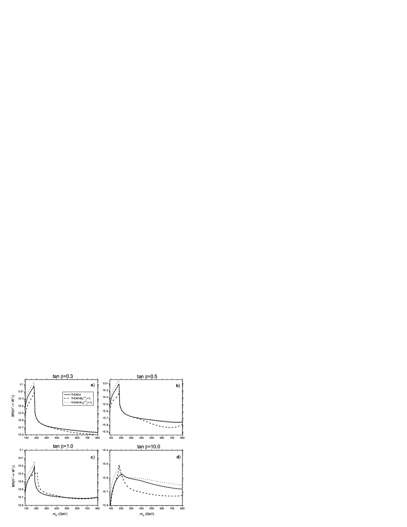
Figure 4: The figure shows the BR$(H^{+}\to W^{+}\gamma)_{\rm III},\,{\rm BR}(H^{+}\to W^{+}\gamma)_{\rm II}$ vs. $m_{H^{+}}$, taking $\tan\beta=0.3,\,0.5,\,1,\,10$ for $\tilde{\chi}_{ij}^{u,d}=-1$ (dots), $\tilde{\chi}_{ij}^{u,d}=0$ or case 2HDM-II (solid line), $\tilde{\chi}_{ij}^{u,d}=1$ (dashes).

IV Events rates at LHC from the decay $H^{+}\to W^{+}\gamma$

The production of charged Higgs bosons at hadron colliders has been evaluated in mapaetal ; diaz-sampayo (also for the Superconducting Super Collider, SSC) and more recently newhcprod ; DiazCruz:2009ek (for the LHC) literature, mainly for the 2HDM-II and its SUSY realization (i.e., the MSSM). In these two scenarios, when kinematically allowed, the top quark decay channel $t\to bH^{+}$ is the dominant $H^{\pm}$ production mechanism. Instead, above the threshold for such a decay, the dominant $H^{\pm}$ production reaction is gluon-gluon fusion into a 3-body final state, i.e., $gg\to tbH^{\pm}$. Both processes depend on the coupling $H^{-}t\bar{b}$ and are therefore sensitive to the modifications that arise in the 2HDM-III for this vertex. However, detection of the final state will depend on the charged Higgs boson decay mode, which could include a complicated final state, that could in turn be difficult to reconstruct. For these reasons, it is very important to look for other production channels, which may be easier to reconstruct. In this regard, the $s$-channel production of charged Higgs bosons, through the mechanism of $c\bar{b}$-fusion, could help to make more viable the detection of several charged Higgs boson decay channels He:1998ie .

IV.1 Evaluation of event rates from direct production of charged Higgs bosons at the LHC

The $H^{\pm}\bar{q}q^{\prime}$ vertex with large flavor mixing coupling, that arises in the 2HDM-III, enables the possibility of studying the production of charged Higgs boson via the $s$-channel production mechanism, $c\bar{b}\to H^{+}$ + c.c. This process was discussed first in Ref. He:1998ie and recently by DiazCruz:2009ek in the context of the 2HDM-III.

To illustrate the type of charged Higgs signatures that have the potential to be detectable at the LHC in the 2HDM-III, we show in the Table 1 the event rates of charged Higgs boson through the channel $c\bar{b}\to H^{+}$ + c.c., alongside the corresponding production cross sections ($\sigma$’s) and relevant BR($H^{+}\to W^{+}\gamma$), for a combination of masses, $\tan\beta$ and specific 2HDM-III parameters amongst those used in the previous sections (assuming $m_{h^{0}}=120$ GeV, $m_{A^{0}}=300$ GeV and the mixing angle at $\alpha=\pi/2$ throughout). In particular, we focus on those cases where the charged Higgs boson mass is above the threshold for $t\to bH^{+}$, for two reasons. On the one hand, the scope of the LHC in accessing $t\to bH^{+}$ decays has been established in a rather model independent way. On the other hand, we have dealt at length with the corresponding BRs in section III. (As default, we also assume an integrated luminosity of $10^{5}$ pb^-1.) In all cases we use the results of our previously work DiazCruz:2009ek .

To illustrate these results, let us comment on one case within the scenario B, because is the case most conservative. From Table 1, we can see that for Scenario B, with $(\tilde{\chi}_{ij}^{u}=1,\tilde{\chi}_{ij}^{d}=1)$ and $\tan\beta=0.3$, we have that the ${H^{\pm}}$ is heavier than $m_{t}-m_{b}$, as we take a mass $m_{H^{+}}=200$ GeV, thus precluding top decay contributions, so that in this case $\sigma(pp\to H^{+}X)\approx 2.2\times 10^{-2}$ pb, and including the decay $H^{+}\to W^{+}\gamma$ , in the final state we set 42 events. Even for charged Higgs masses as long as $300$ GeV, we can still obtain 4 events. The most promising rate for decay $H^{+}\to W^{+}\gamma$, is for $m_{H^{+}}=200$ and $\tan\beta=1$, when we get 63 events.

Table 1: Summary of LHC event rates for some parameter combinations within Scenarios B with an integrated luminosity of $10^{5}$ pb^-1, for the signal $H^{+}\to W^{+}\gamma$, through the channel $c\bar{b}\to H^{+}$ + c.c.

$(\tilde{\chi}_{ij}^{u},\tilde{\chi}_{ij}^{d})$	$\tan\beta$	$m_{H^{+}}$ in GeV	$\sigma(pp\to H^{+}+X)$ in pb	$BR(H^{+}\to W^{+}\gamma)$	Nr. Events
(1,1)	0.3	200	$2.1\times 10^{2}$	$2\times 10^{-6}$	42
(1,1)	0.3	300	$3.1\times 10$	$1.1\times 10^{-6}$	4
(1,1)	1	200	$3$	$2.1\times 10^{-4}$	63
(1,1)	1	300	$0.98$	$4.2\times 10^{-7}$	0
(1,1)	10	200	$1.1$	$9.8\times 10^{-5}$	10
(1,1)	10	300	$5.2\times 10^{-1}$	$1.1\times 10^{-6}$	0

IV.2 Indirect production of charged Higgs bosons at the LHC

We have found that, in some of the 2HDM-III scenarios envisaged here, light charged Higgs bosons could exist that have not been excluded by current experimental bounds, chiefly from LEP2 and Tevatron. Their discovery potential should therefore be studied in view of the upcoming LHC and we shall then turn our attention now to presenting the corresponding hadro-production cross sections via an indirect channel, i.e., other than as secondary products in (anti)top quark decays and via $c\bar{b}$-fusion, considered previously.

In previously work DiazCruz:2009ek , we evaluate the $q\bar{q},gg\to t\bar{b}H^{-}$ + c.c. cross sections. We use HERWIG version 6.510 in default configuration, by onsetting the subprocess IPROC = 3839, wherein we have overwritten the default MSSM/2HDM couplings and masses with those pertaining to the 2HDM-III: see Eqs. (7)–(II).

Now, let discuss again the scenario B. From Table 2, we can see that for this scenario, with $(\tilde{\chi}_{ij}^{u}=1,\tilde{\chi}_{ij}^{d}=1)$ and $\tan\beta=0.3$, we have that the ${H^{\pm}}$ is heavier than $m_{t}-m_{b}$, as we take a mass $m_{H^{+}}=200$ GeV, thus precluding top decay contributions, so that in this case $\sigma(pp\to t\bar{b}H^{-})\approx 25.8$ pb, while the signal $H^{+}\to W^{+}\gamma$ give a number of events of 5. When the mass of the charged Higgs take the value of $300$ GeV, we can obtain only 1 event. One can see that for $m_{H^{+}}=200$ and $\tan\beta=1$, we get 48 events. However, the case most promising rate for decay $H^{+}\to W^{+}\gamma$ is when $m_{H^{+}}=200$ and $\tan\beta=10$, we get the spectacular 122 events, which could be important for the LHC collider experiments.

Altogether, by comparing the $q\bar{q},gg\to t\bar{b}H^{-}$ + c.c. cross sections herein with, e.g., those of the MSSM in Djouadi:2005gj or the 2HDM in Moretti:2002ht ; Moretti:2001pp , it is clear that the 2HDM-III rates can be very large and thus the discovery potential in ATLAS and CMS can be substantial, particularly for a very light $H^{\pm}$, which may pertain to our 2HDM-III but not the MSSM or 2HDM-II. However, it is only by combining the production rates of this section with the decay ones of the previous ones that actual event numbers at the LHC can be predicted.

Table 2: Summary of LHC event rates for some parameter combinations within Scenarios B with for an integrated luminosity of $10^{5}$ pb^-1, for $H^{+}\to W^{+}\gamma$ signature, through the channel $q\bar{q},gg\to\bar{t}bH^{+}$ + c.c.

$(\tilde{\chi}_{ij}^{u},\tilde{\chi}_{ij}^{d})$	$\tan\beta$	$m_{H^{+}}$ in GeV	$\sigma(pp\to H^{+}\bar{t}b)$ in pb	BR$(H^{+}\to W^{+}\gamma)$	Nr. Events
(1,1)	0.3	200	25.8	$2\times 10^{-6}$	5
(1,1)	0.3	300	10.1	$1.1\times 10^{-6}$	1
(1,1)	1	200	2.3	$2.1\times 10^{-4}$	48
(1,1)	1	300	0.79	$4.2\times 10^{-7}$	0
(1,1)	10	200	12.5	$9.8\times 10^{-5}$	122
(1,1)	10	300	$0.48$	$1.1\times 10^{-6}$	0

V Conclusions

We have discussed the implications of assuming a four-zero Yukawa for the properties of the charged Higgs boson, within the context of a 2HDM-III. In particular, we have presented a detailed discussion of the charged Higgs boson couplings to heavy fermions and the resulting implications for the decay $H^{+}\to W^{+}\gamma$, induced at one-loop level. The latter clearly reflect the different coupling structure of the 2HDM-III, e.g., with respect to the 2HDM-II, so that one has at disposal more possibilities to search for $H^{\pm}$ states at current and future colliders, enabling us to distinguish between different models of EWSB. We have then concentrated our analysis to the case of the LHC and showed that the production rates of charged Higgs bosons at the LHC is sensitive to the modifications of the Higgs boson couplings. We have employed the results of the $s$-channel production of $H^{\pm}$ through $c\bar{b}$-fusion and the multibody final state induced by $gg$-fusion and $q\bar{q}$-annihilation. Finally, we have determined the number of events for the most promising LHC signatures for the decay $H^{+}\to W^{+}\gamma$ within 2HDM-III, for both $c\bar{b}\to H^{+}$ + c.c. and $q\bar{q}\to\bar{t}bH^{+}$ + c.c. scatterings (the latter affording larger rates than the former). Armed with these results, we are now in a position to carry out a detailed study of signal and background rates, in order to determine the precise detectability level of each signature. However, this is beyond the scope of present work and will be the subject of a future publication.

References

- (1) S. L. Glashow, Nucl. Phys. 22, 579 (1961); S. Weinberg, Phys. Rev. Lett. 19, 1264 (1967); A. Salam, Proc. 8th NOBEL Symposium, ed. N. Svartholm (Almqvist and Wiksell, Stockholm, 1968), p. 367.
- (2) S. Dawson et al., The Higgs Hunter’s Guide, 2nd ed., Frontiers in Physics Vol. 80 (Addison-Wesley, Reading MA, 1990).
- (3) M. Carena et al., Report of the Tevatron Higgs working group; FERMILAB-CONF-00-279-T; hep-ph/0010338; C. Balazs et al., Phys. Rev. D59, 055016 (1999).
- (4) J.L. Díaz-Cruz et al., Phys. Rev, Lett. 80, 4641 (1998).
- (5) J. Lorenzo Diaz Cruz, AIP Conf. Proc. 1026, 30 (2008).
- (6) A. Djouadi, Phys. Rept. 459, 1 (2008).
- (7) V. D. Barger, J. L. Hewett and R. J. N. Phillips, Phys. Rev. D 41, 3421 (1990).
- (8) See for instance: B. Dobrescu, Phys. Rev. D63, 015004 (2001). See also, recent work on Little Higgs models: N. Arkani-Hamed, A. G. Cohen, E. Katz and A. E. Nelson, JHEP 0207, 034 (2002). And for AdS/CFT Higgs models: R. Contino, Y. Nomura and A. Pomarol, Nucl. Phys. B 671, 148 (2003); A. Aranda, J. L. Diaz-Cruz, J. Hernandez-Sanchez and R. Noriega-Papaqui, Phys. Lett. B 658, 57 (2007)
- (9) J. Brau et al. [ILC Collaboration], arXiv:0712.1950 [physics.acc-ph]; A. Djouadi, J. Lykken, K. Monig, Y. Okada, M.J. Oreglia and S. Yamashita, arXiv:0709.1893 [hep-ph]; T. Behnke et al. [ILC Collaboration], arXiv:0712.2356 [physics.ins-det].
- (10) G. Guignard (editor) [The CLIC Study Team], preprint CERN-2000-008 (2000).
- (11) S. Kanemura, S. Moretti, Y. Mukai, R. Santos and K. Yagyu, arXiv:0901.0204 [hep-ph].
- (12) K. S. Babu and C. F. Kolda, Phys. Lett. B 451, 77 (1999).
- (13) J. L. Diaz-Cruz, R. Noriega-Papaqui and A. Rosado, Phys. Rev. D 71, 015014 (2005).
- (14) J. L. Diaz-Cruz, J. Hernandez-Sanchez, S. Moretti, R. Noriega-Papaqui and A. Rosado, Phys. Rev. D 79, 095025 (2009) [arXiv:0902.4490 [hep-ph]].
- (15) H. Fritzsch and Z. Z. Xing, Phys. Lett. B 555 (2003) 63.
- (16) T. P. Cheng and M. Sher, Phys. Rev. D 35, 3484 (1987).
- (17) J. L. Diaz-Cruz, R. Noriega-Papaqui and A. Rosado, Phys. Rev. D 69, 095002 (2004).
- (18) J. L. Díaz-Cruz and M.A. Pérez, Phys. Rev. D 33, 273 (1986); J. Gunion, G. Kane and J. Wudka, Nucl. Phys. B 299, 231 (1988); A. Mendez and A. Pomarol, Nucl. Phys. B 349, 369 (1991); E. Barradas et al., Phys. Rev. D 53, 1678 (1996); M. Capdequi Peyranere, H. E. Haber and P. Irulegui, Phys. Rev. D 44, 191 (1991); S. Moretti and W. J. Stirling, Phys. Lett. B 347, 291 (1995) [Erratum-ibid. B 366, 451 (1996)]; A. Djouadi, J. Kalinowski and P. M. Zerwas, Z. Phys. C 70, 435 (1996); S. Kanemura, Phys. Rev. D 61, 095001 (2000); E. Asakawa, S. Kanemura and J. Kanzaki, Phys. Rev. D 75, 075022 (2007); A. Arhrib, R. Benbrik and M. Chabab, J. Phys. G 34, 907 (2007); A. Arhrib, R. Benbrik and M. Chabab, Phys. Lett. B 644, 248 (2007).
- (19) J. Hernandez-Sanchez, M. A. Perez, G. Tavares-Velasco and J. J. Toscano, Phys. Rev. D 69, 095008 (2004) [arXiv:hep-ph/0402284].
- (20) J. L. Díaz-Cruz, J. Hernández-Sánchez and J.J. Toscano, Phys. Lett. B 512, 339 (2001).
- (21) J. L. Diaz-Cruz, J. Hernandez-Sanchez, S. Moretti and A. Rosado, Phys. Rev. D 77, 035007 (2008) J. L. Diaz-Cruz, J. Hernandez-Sanchez, S. Moretti and A. Rosado, AIP Conf. Proc. 1026, 138 (2008).
- (22) E. Barradas-Guevara, O. Félix-Beltrán, J. Hernández-Sánchez and A. Rosado, Phys. Rev. D 71, 073004 (2005).
- (23) M. A. Pérez and A. Rosado, Phys. Rev. D 30, 228 (1984); J. Gunion et al., Nucl. Phys. B 294, 621 (1987); J. F. Gunion, Phys. Lett. B 322, 125 (1994).
- (24) J. L. Díaz-Cruz and O.A. Sampayo, Phys. Rev. D 50, 6820 (1994).
- (25) S. Moretti and K. Odagiri, Phys. Rev. D 55, 5627 (1997); Phys. Rev. D 59, 055008 (1999); F. Borzumati, J.-L. Kneur and N. Polonsky, Phys. Rev. D 60, 115011 (1999); S. Moretti and D. P. Roy, Phys. Lett. B 470, 209 (1999); D.J. Miller, S. Moretti, D.P. Roy and W.J. Stirling, Phys. Rev. D61, 055011 (2000); A. A. Barrientos Bendezu and B. A. Kniehl, Phys. Rev. D 59, 015009 (1999); Phys. Rev. D 61, 097701 (2000); Phys. Rev. D 63, 015009 (2001); O. Brein and W. Hollik, Eur. Phys. J. C 13, 175 (2000); O. Brein, W. Hollik and S. Kanemura, Phys. Rev. D 63, 095001 (2001); M. Bisset, M. Guchait and S. Moretti, Eur. Phys. J. C 19, 143 (2001); Z. Fei et al., Phys. Rev. D 63, 015002 (2001); A. Belyaev, D. Garcia, J. Guasch and J. Sola, JHEP 0206, 059 (2002); Phys. Rev. D 65, 031701 (2002); M. Bisset, F. Moortgat and S. Moretti, Eur. Phys. J. C 30, 419 (2003); Q. H. Cao, S. Kanemura and C. P. Yuan, Phys. Rev. D 69, 075008 (2004); E. Asakawa, O. Brein and S. Kanemura, Phys. Rev. D 72, 055017 (2005); E. Asakawa and S. Kanemura, Phys. Lett. B 626, 111 (2005).
- (26) A. Abulencia et al. [CDF Collaboration], Phys. Rev. Lett. 96, 042003 (2006).
- (27) For a review see: F. Borzumati and A. Djouadi, Phys. Lett. B 549, 170 (2002); D. P. Roy, Mod. Phys. Lett. A 19, 1813 (2004).
- (28) C. Amsler et al. [Particle Data Group], Phys. Lett. B 667, 1 (2008).
- (29) S. Kanemura, T. Kubota and E. Takasugi, Phys. Lett. B 313, 155 (1993); J. Horejsi and M. Kladiva, Eur. Phys. J. C 46, 81 (2006); A. G. Akeroyd, A. Arhrib and E. M. Naimi, Phys. Lett. B 490, 119 (2000).
- (30) H. J. He and C. P. Yuan, Phys. Rev. Lett. 83, 28 (1999).
- (31) B. Dudley and C. Kolda, arXiv:0901.3337 [hep-ph].
- (32) F. Borzumati and C. Greub, Phys. Rev. D 59, 057501 (1999).
- (33) Z. J. Xiao and L. Guo, Phys. Rev. D 69, 014002 (2004).
- (34) N. G. Deshpande, P. Lo, J. Trampetic, G. Eilam and P. Singer, Phys. Rev. Lett. 59, 183 (1987).
- (35) D. Bowser-Chao, K. m. Cheung and W. Y. Keung, Phys. Rev. D 59, 115006 (1999) [arXiv:hep-ph/9811235].
- (36) A. Wahab El Kaffas, P. Osland and O. M. Ogreid, Phys. Rev. D 76, 095001 (2007) [arXiv:0706.2997 [hep-ph]].
- (37) G. Isidori, arXiv:0710.5377 [hep-ph].
- (38) J. L. Diaz-Cruz et al., in preparation.
- (39) F. Mahmoudi and O. Stal, arXiv:0907.1791 [hep-ph].
- (40) P. H. Chankowski, M. Krawczyk and J. Zochowski, Eur. Phys. J. C 11, 661 (1999) [arXiv:hep-ph/9905436].
- (41) K. Fujikawa, Phys. Rev. D 7, 393 (1973); M. Bace and N. D. Hari Dass, Ann. Phys. (NY) 94, 349 (1975); M. B. Gavela, G. Girardi, C. Malleville, and P. Sorba, Nucl. Phys. B193, 257 (1981); N. M. Monyonko, J. H. Reid, and A. Sen, Phys. Lett. B 136, 265 (1984); N. M. Monyonko and J. H. Reid, Phys. Rev. D 32, 962 (1985); J. M. Hernández, M. A. Pérez, G. Tavares-Velasco, and J. J. Toscano, Phys. Rev. D 60, 013004 (1999).
- (42) G. Passarino and M. Veltman, Nucl. Phys. B160, 151 (1979).
- (43) G. J. van Oldenborgh, J. A. M. Vermaseren, Z. Phys. C 46, 425 (1990); T. Hahn and M. Pérez-Victoria, Comput. Phys. Commun. 118, 153 (1999).
- (44) S. Moretti, Pramana 60, 369 (2003).
- (45) S. Moretti, J. Phys. G 28, 2567 (2002).