Abstract

General relativity promotes space-time to a physical, dynamical object subject to equations of motion. Quantum gravity, accordingly, must provide a quantum framework for space-time, applicable on the smallest distance scales. Just like generic states in quantum mechanics, quantum space-time structures may be highly counter-intuitive. But if low-energy effects can be extracted, they shed considerable light on the implications to be expected for a dynamical quantum space-time. Loop quantum gravity has provided several such effects, but even in the symmetry-reduced setting of loop quantum cosmology no complete picture of effective space-time geometries describing especially the regime near the big bang has been obtained. The overall situation regarding space-time structures and cosmology is reviewed here, with an emphasis on the role of dynamical states, effective equations, and general covariance.

1 Introduction

In modern cosmology, according to the common scenarios, one is using the universe and its own expansion as a microscope aimed at the smallest distance scales of space and time. In order to understand the resulting phenomena to be expected, the nature of the correct microscopic degrees of freedom, out of which space-time and its dynamics is to emerge, must be understood. There are no direct observations to guide us, and so we are required to make use of further input, of principles that are strong enough to support a large theoretical edifice.

A well-known example for the theoretical derivation of new microscopic degrees of freedom from an underlying principle is the electroweak theory. One of its motivations was a well-defined description of $\beta$-decay, a reaction of four particles (seen at least via the energy carried away in the case of the neutrino). As a pointlike interaction between the four particles involved, the perturbative quantum field theoretical description does not lead to well-defined decay rates. A new principle, renormalizability, is used to look for a more suitable theoretical framework. Its implementation requires the inclusion of new quantum degrees of freedom, the exchange bosons of the electroweak theory. Based on the principle of renormalizability, they were predicted theoretically well before direct observations by particle accelerators became possible.

In quantum gravity, we are currently in a situation similar to that before the direct detection of the exchange bosons. We do not have direct evidence for the microscopic degrees of freedom of quantum gravity, but we do know several problems of the classical theory, chiefly the singularity problem of general relativity. Again, extra input for a theoretical description is needed in the form of principles. One may decide to use those already tried and true, such as renormalizability in this case leading to string theory (as per current understanding). In this way, a quantization of gravitational (and other, unified) excitations on space-time becomes possible. There are, however, difficulties in the description of strong gravitational fields, as we find them at the big bang or in black holes. The interaction of matter with the space-time structure is relevant in those regimes, and so we must consider the quantum nature of full space-time. While this is not impossible in string theory, the theory’s setup makes the analysis of such questions rather indirect.

An alternative principle offers itself, based on what we know about regimes of strong gravitational fields: the principle of background independence. It states the requirement of quantizing the full metric $g_{\mu\nu}$ known as the representative of space-time geometry as it must emerge at large distances or low energies; it is not enough to just quantize perturbations $h_{\mu\nu}$ on a given (e.g. Minkowskian) background where $g_{\mu\nu}=\eta_{\mu\nu}+h_{\mu\nu}$. If only $h_{\mu\nu}$ is quantized and $\eta_{\mu\nu}$ kept as a classical metric background, the theory does not describe the complete space-time geometry in a quantized way. There will be physical quantum degrees of freedom for $h_{\mu\nu}$, but a classical, rigid background $\eta_{\mu\nu}$ remains in the theory. It may be possible to find observables insensitive to which $\eta_{\mu\nu}$ is used, but this would be difficult to achieve and to demonstrate. Moreover, regimes of strong gravitational fields, especially near classical singularities, do not allow a perturvative treatment with a small $h_{\mu\nu}$: The metric becomes degenerate, and so at least some of the crucial components of $h_{\mu\nu}$ are as large as those of $\eta_{\mu\nu}$. Here, a background independent quantization of the full $g_{\mu\nu}$ becomes most useful, a treatment realized in loop quantum gravity.

2 Background independence

Quantum field theory on a background Minkowski space-time may be formulated by operators $a_{\bf k}$ and $a_{\bf k}^{\dagger}$ that describe the annihilation and creation of particles of momentum ${\bf k}$. Using $a_{\bf k}^{\dagger}$ introduces a new particle and increases the total energy, while products of operators in a Hamiltonian amount to interactions. One problem to be faced in quantum gravity is that particles can only be created on a given space-time, whose metric is used in the very definition of $a_{\bf k}$ and $a_{\bf k}^{\dagger}$. A possible solution is to define operators for space-time itself. Such operators would increase distances, areas and volumes; not energy.

Loop quantum gravity [1, 2, 3] provides a specific realization of this solution, at least for spatial geometry. Creation operators turn out to be holonomies [4] $h_{I}={\cal P}\exp(\smallint_{e_{I}}{\rm d}t\dot{e}_{I}^{a}A_{a}^{j}\tau_{j})$ along spatial curves $e_{I}$, evaluated for a connection $A_{a}^{j}=\Gamma_{a}^{j}+\gamma K_{a}^{j}$ called the Ashtekar–Barbero connection [5, 6]. The structure group of the theory is SO(3), referred to by the index $j$ and geometrically corresponding to local spatial rotations. (The matrices $\tau_{j}=-\frac{1}{2}i\sigma_{j}$ are generators of su(2), proportional to the Pauli matrices $\sigma_{j}$.) In the definition of the connection, we use the spatial spin connection $\Gamma_{a}^{i}$ and extrinsic curvature $K_{a}^{i}$, with the Barbero–Immirzi parameter $\gamma>0$ [6, 7], whose value parameterizes a family of canonical transformations. Classically, the connection is canonically conjugate to a densitized vector field $E^{a}_{i}$, the densitized triad related to the spatial metric $q_{ab}$ by $E^{a}_{i}E^{b}_{j}=\det qq^{ab}$: $\{A_{a}^{i}(x),E^{b}_{j}(y)\}=8\pi\gamma G\delta_{a}^{b}\delta^{i}_{j}\delta(x,y)$. This field determines the (torsion-free) spin connection

$$\Gamma_{a}^{i}=-\epsilon^{ijk}e^{b}_{j}(\partial_{[a}e_{b]}^{k}+{\textstyle\frac{1}{2}}e_{k}^{c}e_{a}^{l}\partial_{[c}e_{b]}^{l})\,.$$ (1)

Only the extrinsic curvature part of $A_{a}^{i}$ is independent of the triad.

To start setting up the connection representation for a quantum formulation, we define a basic state $|0\rangle$ by $\langle A_{a}^{i}|0\rangle=1$, fully independent of the connection. A basis of states is obtained by using holonomies as creation operators, which in the simplified U(1)-example (where $h_{e}=\exp(i\int_{e}{\rm d}t\dot{e}^{a}A_{a})$) can be written as

$$|e_{1},k_{1};\ldots;e_{I},k_{I}\rangle=\hat{h}_{e_{1}}^{k_{1}}\cdots\hat{h}_{e_{I}}^{k_{I}}|0\rangle\,.$$

Similar, though more tedious formulas apply for the SU(2)-case of quantum gravity, whose states can be expanded in terms of spin networks [8]. A general state is labeled by a graph $g$ with integers $k_{e}$ as quantum numbers on its edges $e$:

$$\psi_{g,k}(A_{a})=\prod_{e\in g}h_{e}(A_{a})^{k_{e}}=\prod_{e\in g}\exp(ik_{e}\smallint_{e}{\rm d}t\dot{e}^{a}A_{a})\,.$$

Holonomies $h_{I}$ create quantum-gravity states by excitations of two types. (i) one can use operators several times for the same curve, or (ii) use different curves. In this way, an irregular lattice, or spin network, arises which intuitively can be seen as the microscopic structure of space. For a macroscopic geometry, a dense mesh, or strong excitations of the quantum gravity state, are necessary; in order to model near-continuum geometries for which general relativity may approximately apply, one has to consider “many-particle” states.

In order to extract geometrical notions from the visualization of states, operators representing the densitized triad must be introduced. From the densitized triad, the spatial metric and then usual geometrical quantities result [9, 10, 11]. As we had to integrate the connection along curves to obtain holonomies, the densitized triad must be integrated 2-dimensionally in order to obtain well-defined operators: the fluxes $\int_{S}{\rm d}^{2}yE^{a}n_{a}$ integrated over spatial surfaces $S$ with the metric-independent co-normal $n_{a}$ (again written here for the U(1)-simplification). Obtained from momenta conjugate to the connection, fluxes are quantized to derivative operators. Their specific action shows that they measure the excitation level of a state along edges intersecting the surface:

$$\int_{S}{\rm d}^{2}yn_{a}\hat{E}^{a}\psi_{g,k}=8\pi\gamma G\int_{S}{\rm d}^{2}yn_{a}\frac{\hbar}{i}\frac{\delta\psi_{g,k}}{\delta A_{a}(y)}=8\pi\gamma\ell_{\rm P}^{2}\sum_{e\in g}k_{e}{\rm Int}(S,e)\psi_{g,k}$$

with the intersection number ${\rm Int}(S,e)$ and the Planck length $\ell_{\rm P}=\sqrt{G\hbar}$. This is an eigenvalue equation with discrete eigenvalues read off as $8\pi\gamma\ell_{\rm P}^{2}\sum_{e\in g}n_{e}{\rm Int}(S,e)$, and so spatial geometry, represented by the fluxes, is discrete in this framework. The graphs obtained from elementary excitations represent the atomic nature of space, and geometry results from intersections.

In order to see how discrete spatial structures of this kind evolve, dynamics must be introduced. For gravity, this is determined by the Hamiltonian constraint, the phase space functional

$$C_{\rm grav}[N]=\frac{1}{16\pi\gamma G}\int_{\Sigma}\mathrm{d}^{3}xN\left(\epsilon_{ijk}F_{ab}^{i}\frac{E^{a}_{j}E^{b}_{k}}{\sqrt{|\det E|}}-2(1+\gamma^{-2})(A_{a}^{i}-\Gamma_{a}^{i})(A_{b}^{j}-\Gamma_{b}^{j})\frac{E^{[a}_{i}E^{b]}_{j}}{\sqrt{|\det E|}}\right)$$

in Ashtekar variables. In addition to the fields already introduced, we use the curvature $F_{ab}^{i}$ of $A_{a}^{i}$ and the lapse function $N$. As a constraint, $C_{\rm grav}[N]$ must vanish for all choices of $N$.

There are several apparent obstacles in turning this expression into an operator, using the basic holonomies and fluxes. First, an inverse determinant of the densitized triad is required but seems problematic at the operator level, where fluxes, with discrete spectra containing zero, lack densely-defined inverse operators. Nevertheless, as shown by [12], the quantity needed can be obtained from a relation such as

$$\left\{A_{a}^{i},\int{\sqrt{|\det E|}}\mathrm{d}^{3}x\right\}=2\pi\gamma G\epsilon^{ijk}\epsilon_{abc}\frac{E^{b}_{j}E^{c}_{k}}{{\sqrt{|\det E|}}}$$ (2)

whose left-hand side is free of inverses. The volume operator, made from fluxes, can be used for $\int\sqrt{|\det E|}\mathrm{d}^{3}x$, $A_{a}^{i}$ can be expressed in terms of holonomies, and the Poisson bracket is finally turned into a commutator divided by $i\hbar$.

Similarly, the curvature components $F_{ab}^{i}$ of the Ashtekar connection can be expressed in terms of holonomies using identities such as $s_{1}^{a}s_{2}^{b}F_{ab}^{i}\tau_{i}=\Delta^{-1}(h_{\lambda}-1)+O(\Delta)$, where $\lambda$ is a square loop of small coordinate area $\Delta$, with tangent vectors $s_{I}^{a}$ at one of its corners. Finally, extrinsic curvature components $K_{a}^{i}=\gamma^{-1}(A_{a}^{i}-\Gamma_{a}^{i})$, the most complex expressions in the Hamiltonian constraint owing to the spin connection (1) as a functional of the densitized triad, can be obtained from what has already been constructed:

$$K_{a}^{i}=\gamma^{-1}(A_{a}^{i}-\Gamma_{a}^{i})\propto\left\{\!A_{a}^{i},\!\left\{\int{\rm d}^{3}xF_{ab}^{i}\frac{\epsilon^{ijk}E^{a}_{j}E^{b}_{k}}{\sqrt{|\det E|}},\int{\sqrt{|\det E|}}\mathrm{d}^{3}x\right\}\!\!\right\}\,.$$

In this way, a well-defined class of Hamiltonian constraint operators arises, parameterized by certain ambiguities as they arise in the choices to be made. Examples for ambiguities are the exact rewriting of the inverse determinant, or routings and representations for the holonomies used. In spite of ambiguities, several characteristic properties can be extracted and evaluated phenomenologically. In particular, there are three main sources of quantum corrections:

• Inverse volume corrections arise from quantizing the inverse triad determinant in an indirect manner. Comparing eigenvalues of the resulting operators quantizing the left hand side of (2) with the expressions expected from simply inserting flux eigenvalues into the right hand side of (2) shows strong deviations for small flux scales; see Fig. 1

• Higher order corrections result from the use of holonomies, contributing higher powers of the connection components.

• As in any interacting quantum field theory, quantum back-reaction results from the influence of quantum variables such as fluctuations, correlations or higher moments of a state on the expectation values. These variables provide extra degrees of freedom, which can sometimes be interpreted in the sense of higher derivative terms.

Figure 1: Inverse triad correction function, depending on an ambiguity parameter $r$. All curves approach the classical expectation one from above for large flux values $\mu$. (See [13, 14] for explicit derivations of correction functions.)

A simplified form of the Hamiltonian, as it arises from the general constructions of [15, 12], is

$$\hat{C}_{\rm grav}[N]=\frac{i}{16\pi\gamma G\hbar}\sum_{v,IJK}N(v)\sum_{\sigma_{I}\in\{\pm 1\}}\sigma_{1}\sigma_{2}\sigma_{3}\epsilon^{IJK}{\rm tr}(h_{v,I}h_{v+I,J}h_{v+J,I}^{-1}h_{v,J}^{-1}h_{v,K}[h_{v,K}^{-1},\hat{V}])$$ (3)

of interacting form: excitations of geometry take place dynamically by the factors of holonomy operators included in the expression. All this depends on the spatial geometry through the volume operator $\hat{V}$. The discreteness contained in the resulting dynamics is significant at high densities (such as the big bang), or if many small corrections add up in a large universe (for dark energy, perhaps).

3 Loop quantum cosmology

In full generality, it is difficult to analyze the dynamics of quantum gravity, but several results are known in model systems (based on symmetry reduction or perturbative inhomogeneities). One can easily imagine simplifications from the considerable reduction of the number of degrees of freedom, but also from another effect: level-splitting, well-known from energy spectra of atoms and molecules. Also in quantum geometry, levels split when symmetries are relaxed, making spectra of symmetric situations much simpler than non-symmetric ones. In particular, the volume spectrum, which despite significant numerical progress [16, 17] is rather difficult to compute in the full case, splits when symmetry is relaxed from homogeneity to spherical symmetry as shown in Fig. 2. The most highly symmetric systems should then the easiest to analyze, also concerning the dynamics. This is the realm of quantum cosmology.

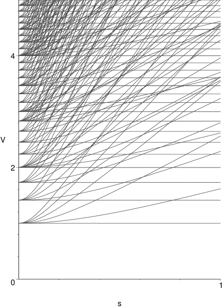
Figure 2: Level splitting of volume eigenvalues as a symmetry parameter $s$ is tuned from zero (homogeneity) to one (spherical symmetry); see [18] for details.

Loop quantum cosmology [19] provides a quantization of symmetry reduced models by the techniques of loop quantum gravity. Many of its ingredients, in particular its states and basic operators, can be induced from the full holonomy-flux algebra [20, 21, 22, 23, 24] or by other means [25, 26]; in this sense loop quantum cosmology is a sector of (kinematical) loop quantum gravity. Just the dynamics, which is problematic and not yet in a settled stage even in the full theory, is too complicated to be reduced directly from a full Hamiltonian constraint such as (3). In formulating the dynamics, based on the basic operators, additional assumptions and extra input are sometimes required and cannot yet be derived from the full theory. This may introduce an amount of ambiguity larger than that already realized in the full theory.

Hamiltonian isotropic cosmology in Ashtekar variables (here written only for spatially flat models), has the basic phase space variables $A_{a}^{i}=c\delta_{a}^{i}$ with $c=\gamma\dot{a}$, $E^{a}_{i}=p\delta^{a}_{i}$ with $|p|=a^{2}$. (For a triad with the option of two different orientations, $p$ can take both signs; see [27] for details of the classical reduction.) The coefficients $c$ of an isotropic connection and $p$ of an isotropic triad are canonically conjugate: $\{c,p\}=8\pi\gamma G/3$. Inserting these reductions into the full Hamiltonian constaint provides

$$C:=-\frac{c^{2}\sqrt{|p|}}{\gamma^{2}}+\frac{8\pi G}{3}H_{\rm matter}=0$$

as the isotropic constraint equation, equivalent to the Friedmann equation. (For homogeneous cosmology, the lapse function $N$ must be spatially constant, thus providing a single constraint function.) The gauge-flow in time, $\dot{p}=\{p,C\}$ and $\dot{c}=\{c,C\}$, generated by the constraint amounts to the Raychaudhuri equation.

In loop quantum cosmology, just as in Wheeler–DeWitt quantum cosmology [28, 29], the constraint is quantized to an operator annihilating physical states: $\hat{C}|\psi\rangle=0$. In contrast to the Wheeler–DeWitt representation, however, the use of $\exp(i\delta c)$ for $c$ — matrix elements of holonomies as required for a background-independent representation — makes us regularize the constraint before it can be quantized. For instance, with an ambiguity parameter $\delta$ (which can and often should be allowed to be a phase-space function; see Sec. 5) we may write

$$-\frac{\sin^{2}(\delta c)\sqrt{|p|}}{\gamma^{2}\delta^{2}}+\frac{8\pi G}{3}H_{\rm matter}=0$$ (4)

as an expression that agrees very well with the classical one for small curvature ($\delta c\ll 1$) and at the same time is quantizable in terms of holonomies. Effects of such a modification easily trickle down to low-curvature equations [30, 31].

Replacing connection components by matrix elements of holonomies constitutes a regularization motivated from quantum geometry via background independence; it is not in itself a quantum effect even if, as sometimes done in improvised versions, $\delta$ is related to $\hbar$ or $\ell_{\rm P}$ by further ad-hoc arguments. Indeed, in a systematic derivation of effective equations describing loop quantum cosmology, (4) is recognized simply as the pure tree-level contribution where all quantum corrections vanish [36, 37]; see also [38, 39] for discussions of the regularization. Although care must always be exercised, using just the regularization allows one to explore the potential consequences of quantum gravity. The regularization is, of course, easy to implement in exactly homogeneous models, and it is far from being unique. The real issues to be faced arise when one tries to extend the regularization to inhomogeneous situations, at least of perturbative nature, in which extremely tight constraints due to covariance arise. Consistent implementations may strongly reduce the ambiguities — and possibly eliminate effects seen in simple homogeneous models. Such issues related to inhomogeneity will be discussed in more detail in Sec. 6.

An immediate implication of using holonomies is that the constraint equation is not differential, but a difference equation for a wave function of the universe [40, 27]. Writing $\hat{C}|\psi\rangle=0$ for a state $|\psi\rangle=\sum_{\mu}\psi_{\mu}(\phi)|\mu\rangle$ expanded in triad eigenstates $|\mu\rangle$ (with an extra collective label $\phi$ for matter fields) requires the coefficients $\psi_{\mu}(\phi)$ to satisfy

$$C_{+}(\mu)\psi_{\mu+\delta}(\phi)-C_{0}(\mu)\psi_{\mu}(\phi)+C_{-}(\mu)\psi_{\mu-\delta}(\phi)=\hat{H}_{\phi}(\mu)\psi_{\mu}(\phi)\,.$$ (5)

All coefficients of this equation can be derived, but are not fixed uniquely owing to the non-uniqueness of the Hamiltonian constraint operator. Nonetheless, several qualitative properties, insensitive to ambiguities, have been found. The left-hand side quantizes the gravitational contribution to the constraint and shows the discreteness, while the right-hand side shows what role is played by the matter Hamiltonian $\hat{H}_{\phi}$. If we view the size variable $\mu$ as an “internal time,” evolution proceeds discretely.

Loop quantum cosmology is non-singular [41]: any wave function evolves uniquely across the classical singularity (situated at $\mu=0$). Quantum hyperbolicity [42] of this form has been realized not only in isotropic models, but also in anisotropic ones [43, 44] and even in some inhomogeneous situations such as spherical symmetry [45]. Physically, one may explain this phenomenon by a limited storage for energy provided in a discrete space-time: Quantum waves must now be supported on a discrete lattice, providing a natural cut-off for wave-lengths. Dynamically, a repulsive force arises once energy densities become too large, counter-acting the classical attraction and preventing singularities.

In simple models in which also the matter content is severely restricted by being close to a free, massless scalar — resulting in an exactly solvable, harmonic model as shown below —, numerical [46] and exact solutions [36] indeed show that the expectation value of the scale factor bounces, reaching a non-zero minimum value. This geometrical picture is, however, not available in strong quantum regimes in which several of the quantum variables matter: a state changes considerably as the big bang is approached or traversed, a dynamical behavior which can no longer be formulated just in terms of the classical variables of geometry (solely the scale factor in isotropic cosmology). To handle such situations, effective equations are useful.

4 Effective equations

To illustrate the derivation of effective equations in canonical quantum systems we start with a simple example from quantum mechanics: the harmonic oscillator. Its dynamics is defined by the closed, linear algebra

$$[\hat{q},\hat{p}]=i\hbar\quad,\quad{}[\hat{q},\hat{H}]=i\hbar\frac{\hat{p}}{m}{}\quad,\quad{}[\hat{p},\hat{H}]=-i\hbar m\omega^{2}\hat{q}$$

of basic operators and the Hamiltonian $\hat{H}$. Any quantum system with such a closed and linear algebra has dynamical solutions whose wave functions may spread, but do so without disturbing the mean position. Indeed, a closed set of equations results for expectation values of $\hat{q}$ and $\hat{p}$ via ${\rm d}\langle\hat{O}\rangle/{\rm d}t=\langle[\hat{O},\hat{H}]\rangle/i\hbar$. To solve these equations, we need not know how fluctuations, correlations or higher moments of the state behave; there is no quantum back-reaction. Similarly, there is a closed set of equations just for the fluctuations and correlations, without coupling to moments of higher than second order.

A similarly solvable system exists in loop quantum cosmology [36, 47], with the conditions of an isotropic, spatially flat space and matter given by a free, massless scalar $\phi$. Using the loop-quantized Hamiltonian (in a particular factor ordering and ignoring inverse volume corrections at this stage) again produces a closed algebra of basic variables, provided we choose them as the volume $V$ (or, more generally, $|p|^{1-x}$ to absorb any $p$-dependence of $\delta$ provided it is a power-law $\delta(p)=\delta_{0}|p|^{x}$) and the holonomy-related quantity $J=V\exp(i\delta_{0}P)$ with the Hubble parameter $P$ (or $|p|^{x}c$) conjugate to $V$. This time, using the Hamiltonian $p_{\phi}\propto h:={\rm Im}J$ with respect to evolution in $\phi$ as internal time, as it follows from the regularized Hamiltonian (4) with $H_{\rm matter}=p_{\phi}^{2}/2a^{3}$, the algebra is sl$(2,{\mathbb{R}})$:

$$[\hat{V},\hat{J}]=-\delta_{0}\hbar\hat{J}\quad,\quad{}[\hat{V},\hat{h}]={\textstyle\frac{1}{2}}i\delta_{0}\hbar(\hat{J}+\hat{J}^{\dagger})\quad,\quad{}[\hat{J},\hat{h}]=i\delta_{0}\hbar\hat{V}\,.$$

(The Hamiltonian constraint for a free, massless scalar field can be written as $p_{\phi}^{2}-VC_{\rm grav}=0$, and easily be deparameterized. One is taking a square root in the process to solve for $p_{\phi}$, but this does not spoil the linearity of the dynamics of states just required to be semiclasical once [47]. Alternatively, direct treatments of effective constraints, avoiding deparameterization, are available [48, 49, 50].)

Equations of motion

$$\frac{{\rm d}\langle\hat{O}\rangle}{{\rm d}\phi}=\frac{\langle[\hat{O},\hat{h}]\rangle}{i\hbar}$$

generated with respect to $\phi$ now provide the behavior of physical observables: There is no absolute time in this fully constrained system; instead, change is measured by relational observables, such as $\langle\hat{V}\rangle(\phi)$ between the degrees of freedom. (For a complete reduction to physical quantities, reality conditions must be imposed to ensure the correct adjointness properties for a quantization of the real $P$ appearing in the complex $J$. Appropriate conditions turn out to be easily formulated, relating expectation values to fluctuations and correlations [47].) Also here, there is no quantum back-reaction in the solvable model. Fluctuations do not back-react on the expectation values, which results in simple, cosh-like solutions for the volume; see Fig. 3. Clearly, the volume never becomes zero, and the singularity, of these specific models, is replaced by a bounce. While the expectation value follows its trajectory undisturbed, states in general do spread. In particular, squeezed states (with non-vanishing correlations) describe oscillating fluctuations between different universe phases, expansion and collapse. As it turns out, fluctuations can change by an order of magnitude even in dynamical coherent states — the most strongly controlled type of states —, and this change is very sensitive to initial values. This cosmic forgetfulness makes it difficult to estimate specific quantities in the pre-bounce phase for realistic models [51, 52].

Figure 3: Bouncing solutions of the exactly solvable model of loop quantum cosmology, showing the expectation value of the physical observable $\langle\hat{V}\rangle(\phi)$, as well as the spread $\Delta V(\phi)$of a physical wave function. The label “$h$” indicates the size of the (conserved) $\phi$-Hamiltonian, which determines the volume at the bounce.

Generic models are more complicated since they are subject to quantum back-reaction. To illustrate this, we consider a model with a cosmological constant, but ignore the quantum geometry corrections of loop quantum cosmology for the sake of simplicity. The Hamiltonian for $\phi$-evolution, as treated for a negative cosmological constant in [53], then is $p_{\phi}\propto V\sqrt{P^{2}-\Lambda}=:h(V,P)$. (The same system was analyzed numerically in [54].) Now, expectation values couple to fluctuations and other moments:

$$\frac{{\rm d}\langle\hat{V}\rangle}{{\rm d}\phi} = \frac{3}{2}\frac{\langle\hat{V}\rangle\langle\hat{P}\rangle}{\sqrt{\langle\hat{P}\rangle^{2}-\Lambda}}+\frac{9}{4}\Lambda\frac{\langle\hat{V}\rangle\langle\hat{P}\rangle}{(\langle\hat{P}\rangle^{2}-\Lambda)^{5/2}}(\Delta P)^{2}-\frac{3}{2}\Lambda\frac{C_{VP}}{(\langle\hat{P}\rangle^{2}-\Lambda)^{3/2}}+\cdots$$

$$\frac{{\rm d}\langle\hat{P}\rangle}{{\rm d}\phi} = -\frac{3}{2}\sqrt{\langle\hat{P}\rangle^{2}-\Lambda}+\frac{3}{4}\Lambda\frac{(\Delta P)^{2}}{(\langle\hat{P}\rangle^{2}-\Lambda)^{3/2}}+\cdots$$

with the $\hat{P}$-fluctuation $\Delta P$ and the covariance $C_{VP}=\frac{1}{2}\langle\hat{V}\hat{P}+\hat{P}\hat{V}\rangle-\langle\hat{V}\rangle\langle\hat{P}\rangle$. Fluctuations are dynamical, too:

$$\frac{{\rm d}(\Delta P)^{2}}{{\rm d}\phi} = -3\frac{\langle\hat{P}\rangle}{\sqrt{\langle\hat{P}\rangle^{2}-\Lambda}}(\Delta P)^{2}+\cdots$$

$$\frac{{\rm d}C_{VP}}{{\rm d}\phi} = -\frac{3}{2}\Lambda\frac{\langle\hat{V}\rangle}{(\langle\hat{P}\rangle^{2}-\Lambda)^{3/2}}(\Delta P)^{2}+\cdots$$

$$\frac{{\rm d}(\Delta V)^{2}}{{\rm d}\phi} = -3\Lambda\frac{\langle\hat{V}\rangle}{(\langle\hat{P}\rangle^{2}-\Lambda)^{3/2}}C_{VP}+3\frac{\langle\hat{P}\rangle}{\sqrt{\langle\hat{P}\rangle^{2}-\Lambda}}(\Delta V)^{2}+\cdots\,.$$

(In all these equations, dots indicate that higher order moments have been ignored here.)

Analyzing coupled equations like this is the canonical procedure for effective equations. (For anharmonic oscillators in quantum mechanics, employing a semiclassical as well as an adiabatic approximation, the usual low-energy effective action is reproduced [55, 56].) Often, higher moments can be ignored in certain regimes, starting with a semiclassical state whose moments of order $n$ are suppressed by a factor of $\hbar^{n/2}$. But long evolution, as is prevalent in cosmology, can drastically change a state even if it starts out semiclassically to a high degree. Moments may then grow, and higher ones will become important. Severe quantum back-reaction effects can be expected, especially in the infamously strong quantum regime around the big bang. But also other regimes exist where large moments are perhaps more surprising. One example is that of the large-volume regime of models with a positive cosmological constant. As can be seen from the preceding equations, several of the coefficients then have denominators that can come close to zero when the curvature scale squared approaches the cosmological constant. For a small, perhaps realistic, cosmological constant, this regime is approached at large volume, where moments can grow large despite the classical appearance of the phase.

The back-reaction equations of loop quantum cosmology are much more lengthy [57], but can be summarized in a quantum Friedmann equation including the effects from holonomy corrections and quantum back-reaction [58, 59]. With a scalar mass or a self-interacting potential, the equation

$$\left(\frac{\dot{a}}{a}\right)^{2}=\frac{8\pi G}{3}\left(\rho\left(1-\frac{\rho_{Q}}{\rho_{\rm crit}}\right)\pm\frac{1}{2}\sqrt{1-\frac{\rho_{Q}}{\rho_{\rm crit}}}\eta(\rho-P)+\frac{(\rho-P)^{2}}{(\rho+P)^{2}}\eta^{2}\right)$$ (6)

describes the evolution of the scale factor’s expectation value. Compared to the classical equation, pressure $P$ enters, as well as $\eta$ which parameterizes quantum correlations. Moreover,

$$\rho_{Q}:=\rho+\epsilon_{0}\rho_{\rm crit}+(\rho-P)\sum_{k=0}^{\infty}\epsilon_{k+1}(\rho-P)^{k}/(\rho+P)^{k}$$

is an expression for a quantum corrected energy density with fluctuation parameters $\epsilon_{k}$, and $\rho_{\rm crit}=3/8\pi G(a\delta)^{2}$ is a critical density with scale $a\delta$ as determined by the $\delta$ used in the regularization (4) by holonomies. The critical density is constant only if $\delta\propto a^{-1}$ (a special case introduced in [60]). The behavior following from this equation is simple if $\rho=p$ (the free, massless scalar case) or if $\rho+p$ is large (large $p_{\phi}$, or kinetic domination). Then, solutions with $\dot{a}=0$ exist near $\rho=\rho_{\rm crit}$, producing a bounce.

For regimes not of kinetic domination, the behavior of many moments, contained in $\eta$ and $\rho_{Q}$, must be known for a precise picture, requiring a long analysis still to be completed. Only such an analysis can show what effective geometrical picture corresponds to the general singularity avoidence by the difference equation of loop quantum cosmology. In particular, it has not been shown that loop quantum cosmology generically replaces the big bang singularity by a bounce.

Currently, all existing indications for bounces — numerical as in [61, 62] or analytic as in [59] — exist only for kinetic-dominated regimes of a scalar matter source. The situation is slightly more general for demonstrating an upper bound of energy density, but such a statement is weaker than showing the existence of bouncing solutions. (Bounces can easily be produced quite generally even in potential-dominated regimes using the tree-level approximation of loop quantum cosmology. However, the tree-level approximation itself does not appear reliable in potential-dominated regimes.)

5 Lattice refinement

Loop quantum cosmology aims to model the dynamical behavior of loop quantum gravity in a tractable manner. Since no procedure is known for a complete reduction of the Hamiltonian constraint to isotropy or homogeneity, several choices are to be made in specifying the Hamiltonian constraint of loop quantum cosmology, giving rise to the difference equation (5). One such freedom concerns the parameter $\delta$ in (4), which may be a phase-space function as alluded to above.

This function carries important information about the reduction [22, 63]. It appears as a coefficient of the connection component in holonomies as used for the dynamics. If we look at the schematic full constraint of (3), it is clear that holonomies in that operator refer to edges in one of the graph states, as it evolves according to the dynamics of loop quantum gravity. Reducing such a holonomy to isotropic variables leads to an expression of the form $\exp(i\delta c)$, exactly as used in the reduced constraint. In the reduced model, $\delta$ appears as a parameter which can only be chosen by hand to have a specific value; no argument has been found to fix it. In the full context, on the other hand, $\delta$ is clearly related to the coordinate length of the edge used, and thus refers to the underlying inhomogeneous state. (Although $\delta$ is coordinate dependent, the combination $\delta c=\gamma\delta\dot{a}$ appearing in holonomies is not.) In the reduction to homogeneity, that information in the state is lost; one can only bring it back by making certain phenomenological choices for $\delta$.

The underlying inhomogeneous state is dynamical: new edges may be created or old ones removed. Edge lengths change, and so does $\delta$. One way to model this in an isotropic description is to allow $\delta$ to depend on the scale factor $a$, implying that the underlying inhomogeneous state changes as the universe expands or contracts. By analyzing the resulting models, phenomenological restrictions for the behavior of $\delta$ can be found [64, 65, 66]. What is so far indicated is that a power-law form of $\delta=\delta_{0}|p|^{x}$ works best for $x$ near $-1/2$.

Lattice refinement has been formulated in a parameterized way for anisotropic models, also at the level of underlying difference equations. Compared to isotropic models, the difference equations then generically become non-equidistant, complicating an analysis. A complete formulation of the dynamics (avoiding ad-hoc assumptions), especially for the Schwarzschild interior but also providing Misner-type variables for Bianchi models, has been provided in [67]. Numerical tools to evaluate non-equidistant difference equations have been introduced in [68, 69].

6 Cosmology

With matter interactions and inhomogeneities, a complicated form of back-reaction results that can be handled only by a systematic perturbation theory around the solvable model. The solvable model of loop quantum cosmology then plays the same role as free quantum field theories do for the Feynman expansion. An analysis of this form can show possible indirect effects of the atomic space-time where individual corrections which are small even at high energies might add up coherently. If this magnification effect is strong enough, one might come close to observability. Two prime examples exist: cosmology, which is a high energy density regime with long evolution times for corrections to add up; and high energy particles from distant sources.

But before one analyzes complete equations — those containing all possible quantum corrections for possible physical consequences — there is an interesting geometrical set of problems related to general covariance. Compared to homogeneous models, where modifications such as those in (4) can consistently be implemented at will, general covariance in inhomogeneous situations is a strong consistency requirement. For instance, the contracted Bianchi identity $\nabla_{\mu}G^{\mu}_{\nu}=0$ implies $\partial_{0}G^{0}_{\mu}=-\partial_{a}G^{a}_{\mu}-\Gamma^{\nu}_{\nu\kappa}G^{\kappa}_{\mu}+\Gamma^{\kappa}_{\mu\nu}G^{\nu}_{\kappa}$ . The right-hand side is at most of second order in time derivatives, and so $G^{0}_{\mu}$ must be of first order. The corresponding components of Einstein’s equation provide constraints for initial values rather than evolution equations:

$$\int{\rm d}^{3}xN(x)\sqrt{\det q}(G^{0}_{0}-8\pi GT^{0}_{0})=0$$ (7)

(with the spatial metric tensor $q_{ab}$ used in the integration measure) and

$$\int{\rm d}^{3}xN^{a}(x)\sqrt{\det q}(G^{0}_{a}-8\pi GT^{0}_{a})=0$$ (8)

where $q_{ab}$ is again the spatial metric. The constraints must be preserved under the second order equations that follow from the spatial components $G^{a}_{b}$.

This kind of conservation law leads to symmetries: We have a scalar constraint $C[N]$, the Hamiltonian constraint, and a vectorial one, the diffeomorphism constraint $D[N^{a}]$, satisfying a closed algebra

$$\{D[N^{a}],D[M^{a}]\} = D[{\cal L}_{M^{a}}N^{a}]$$

$$\{C[N],D[M^{a}]\} = C[{\cal L}_{M^{a}}N]$$

$$\{C[N],C[M]\} = D[q^{ab}(N\partial_{b}M-M\partial_{b}N)]$$

as the generators of gauge transformations. Importantly, this algebra is first class: Poisson brackets of the constraints vanish when the constraints are imposed. On the solution space, constraints are invariant under the flow they generate, and thus provide gauge-invariant equations. In the case of gravity, the combination $C[N]+D[N^{a}]$ generates infinitesimal space-time diffeomorphism along $\xi^{\mu}=(N,N^{a})$, as can be checked by a direct calculation and comparison with Lie derivatives. General covariance can be expressed fully in terms of this algebra, as emphasized by Dirac [70]:

“It would be permissible to look upon the Hamiltonian form as the fundamental one, and there would then be no fundamental four-dimensional symmetry in the theory.

The usual requirement of four-dimensional symmetry in physical laws would then get replaced by the requirement that the functions have weakly vanishing [Poisson brackets].”

Such a viewpoint is convenient especially in canonical quantum gravity. It is not guaranteed that quantization preserves the usual space-time or differential-geometric notions, and that it leads to the same relationship between symmetries and Lie derivatives. In contrast to differential geometry, an algebra of constraints, which will become a commutator algebra of the corresponding operators, can directly be carried over to the quantum theory. In this way, the realization of symmetries, and correspondingly of space-time structures, can be tested at the quantum level. Quantum corrections usually change the constraints as gauge generators and may thus lead to changes in the space-time structures. Also the algebra of constraints may be corrected, but for a consistent formulation, corrections must respect the first-class nature of the algebra. If the first-class nature is respected, symmetries may be deformed but are not lost; the quantum system is then called anomaly-free.

“Effective” constraints, including some of the corrections from quantum geometry (in this case inverse volume corrections), can be made anomaly-free [71]:

$$\{D[N^{a}],D[M^{a}]\} = D[{\cal L}_{M^{a}}N^{a}]$$

$$\{C_{(\alpha)}[N],D[M^{a}]\} = C_{(\alpha)}[{\cal L}_{M^{a}}N]$$

$$\{C_{(\alpha)}[N],C_{(\alpha)}[M]\} = D[\alpha^{2}q^{ab}(N\partial_{b}M-M\partial_{b}N)]$$

where $\alpha$ is the correction function from inverse volume operators. This algebra is indeed first class, but deformed. To interpret the corrections, we first note that in an effective action they cannot be purely of higher curvature type, for such corrections would still produce the classical algebra [72]. We are thus dealing with a more general type of effective action (such as one on a non-commutative space-time). Similar deformations have been constructed for holonomy corrections, although not for the complete case of cosmological perturbations. The first example was found for spherically symmetric models [73] (see also [74, 75]), with a similar form produced for $2+1$-dimensional gravity [76]. (Although the deformations in those two cases are quite similar, there is a difference in that the $2+1$-example requires a non-vanishing cosmological constant for the deformation to appear. This circumstance may just be a consequence of the special form of $2+1$-dimensional gravity in the formulation used, where the theory without a cosmological constant has vanishing on-shell curvature and is topological.) Constructing consistent deformations corresponding to quantum geometry corrections is the non-trivial part of an analysis making simple modifications such as (4) relevant.

Practically, one consequence of the deformation is that the potential size of quantum corrections is larger than often expected, that is larger than $\ell_{\rm P}{\cal H}$ as higher curvature terms would produce it in cosmological situations. The main physical mechanism is non-conservation of power on large scales, modifying an approximate conservation which classically follows very generally from the conservation of stress-energy, or the Bianchi identity; see e.g. [77, 78, 79]. The Bianchi identity, however, takes a different form for the corrected constraint algebra, and so quantum corrections affect large-scale modes, removing the constant one [80, 81]. Local corrections for the slope of increase or decrease of super-Hubble power, for scalar and tensor modes, are small, but realized during long evolution times. They may add up to sizeable effects.

Explicitly, the resulting cosmological perturbation equations (for all scales on a background Friedmann–Robertson–Walker space-time with conformal Hubble rate ${\cal H}$ and the background scalar $\bar{\varphi}$) are [81]

$$\partial_{c}\left(\dot{\Psi}+{\cal H}(1+f)\Phi\right)=4\pi G\frac{\bar{\alpha}}{\bar{\nu}}\dot{\bar{\varphi}}\partial_{c}\delta\varphi$$ (9)

from the diffeomorphism constraint,

$$\Delta(\bar{\alpha}^{2}\Psi)-3{\cal H}(1+f)\left(\dot{\Psi}+{\cal H}\Phi(1+f)\right)=4\pi G\frac{\bar{\alpha}}{\bar{\nu}}(1+f_{3})\left(\dot{\bar{\varphi}}\delta\dot{\varphi}-\dot{\bar{\varphi}}^{2}(1+f_{1})\Phi+\bar{\nu}a^{2}V_{,\varphi}(\bar{\varphi})\delta\varphi\right)$$ (10)

from the Hamiltonian constraint, and

$$\ddot{\Psi}+{\cal H}\left(2\dot{\Psi}\left(1-\frac{a}{2\bar{\alpha}}\frac{{\rm d}\bar{\alpha}}{{\rm d}a}\right)+\dot{\Phi}(1+f)\right)+\left(2\dot{\cal H}+{\cal H}^{2}\left(1+\frac{a}{2}\frac{{\rm d}f}{{\rm d}a}-\frac{a}{2\bar{\alpha}}\frac{{\rm d}\bar{\alpha}}{{\rm d}a}\right)\right)\Phi(1+f)$$ (11)

$$= 4\pi G\frac{\bar{\alpha}}{\bar{\nu}}\left(\dot{\bar{\varphi}}\delta\dot{\varphi}-a^{2}\bar{\nu}V_{,\varphi}(\bar{\varphi})\delta\varphi\right)$$

as the evolution equation. These equations are accompanied by $\Phi=(1+h)\Psi$, which follows from off-diagonal components of the corrected Einstein equation, and a corrected Klein–Gordon equation for $\delta\varphi$. In addition to the gauge-invariant metric perturbations $\Phi$ and $\Psi$ and the scalar perturbation $\delta\varphi$ as well as the primary correction function $\bar{\alpha}$ from inverse volume (and $\bar{\nu}$ for the matter term), several other corrections, $f$, $f_{1}$, $f_{3}$, $h$ arise, but are related to the primary correction.

The consistency issue now becomes a very practical problem: There are five equations for three free functions, $\Phi$, $\Psi$ and $\delta\varphi$. Classically the system is consistent and not overdetermined thanks to general covariance. But will this closure of the equations be preserved in the presence of quantum corrections from discrete geometry? As indicated by the possibility of a first-class (but deformed) algebra of constraints, consistency can be realized. There are no anomalies (checked to linear order in perturbations in [71]) if the quantum correction functions satisfy equations such as

$$-h-f+\frac{a}{\bar{\alpha}}\frac{\partial\bar{\alpha}}{\partial a} = 0\quad,\quad 3f-2a\frac{\partial f}{\partial a}-\frac{a}{\bar{\alpha}}\frac{\partial\bar{\alpha}}{\partial a}=0$$

$$\frac{1}{6}\frac{\partial\bar{\alpha}}{\partial a}\frac{\delta E^{c}_{j}}{a^{3}}+\frac{\partial\alpha^{(2)}}{\partial(\delta E^{a}_{i})}(\delta^{a}_{j}\delta^{c}_{i}-\delta^{c}_{j}\delta^{a}_{i}) = 0\,.$$

The last of these equation relates higher perturbative orders of $\alpha$ to the background value $\bar{\alpha}$ achieved for isotropic geometries. If these equations are satisfied, which is possible even in non-classical cases of $\alpha\not=1$, the whole set of cosmological perturbation equations is consistent. Moreover, all coefficients for quantum corrections are fixed in terms of $\bar{\alpha}$, and this function can be derived in isotropic models (up to ambiguities). Inverse volume corrections, resulting from discrete features of spatial quantum geometry, provide a consistent deformation: The underlying discreteness (for this type of corrections) does not destroy general covariance.

General covariance is a statement about the quantum constraint algebra, and thus can be ensured only by considering perturbation theory without fixing the space-time gauge. After consistent equations have been derived, one may certainly pick a gauge (such as the longitudinal one) if that simplifies calculations. But fixing the gauge before deriving perturbation equations and observables does not verify covariance and can easily lead to spurious effects. Explicit examples can be seen by comparing [82] with [81], the first one with gauge-fixing, the second one without. As turns out, the relationship between the metric perturbations $\Phi$ and $\Psi$ is affected by the treatment, as is the precise form of non-conserved power on large scales. Only without gauge-fixing is it possible to ensure consistency; only those results are reliable. When computing the effects of an underlying discrete space-time structure on inflationary structure formation, or on the propagation of modes through a potential bounce, that kind of consistency is especially important. For evolution through a bounce, no consistent form for scalar modes has been found yet; existing treatments all use gauge-fixing [83, 84, 85].

One of the implications for cosmological scenarios is that quantum geometry corrections (inverse volume or holonomy) often imply super-inflation at high densities [86]. There may not be many e-foldings in terms of $\log(a_{\rm f}/a_{\rm i})$, referring only to the final and initial values of the scale factor (see Fig. 4), but $\log\left((a{\cal H})_{\rm f}/(a{\cal H})_{\rm i}\right)$ can be large due to the growth of ${\cal H}$ during super-inflation [87]. Viable scenarios thus exist, but the degree of fine-tuning has not yet been fully estimated. Regarding details, several analyses have been performed depending on the scalar potential and quantization ambiguities. Unfortunately, perturbation results are currently on a rather weak basis in strong quantum (or high density) regimes since anomaly-free effective equations are difficult to control. For instance, no consistent evolution of scalar modes through the bounce yet exists. Nevertheless, in weaker regimes some parameters, such as the power-law of a scalar potential, can already be constrained (in [88], using WMAP5 data). At the current stage, primordial gravitational waves [89] are under better analytical control since they are not subject to gauge transformation or overdeterminedness. Some implications for the tensor power spectrum have been evaluated in [90, 91, 92, 93, 94, 95, 66].

Figure 4: A bouncing scale factor, with super-inflation between the dotted lines (and the singular classical solution as the dashed line). In this phase, the scale factor varies only by a few percent, but $a{\cal H}$ changes more. The effective solution corresponds to the solvable model as plotted in Fig. 3, transformed to proper time. Similar solutions have been found in [96] directly in proper time.

7 Outlook

Consistent deformations exist in model systems of canonical quantum gravity: discreteness can be realized without spoiling covariance. These results of anomaly freedom show that discrete structures are able to preserve covariance; when realized, they make simple modifications as they are possible in homogeneous models highly non-trivial. So far, this demonstration has been achieved only in relatively tame regimes, but not yet close to the classical big bang singularity, or even through bounce phases.

Examples have been constructed for cosmological perturbations and for black holes. This is mainly based on canonical effective equations, whose tools, analytical as well as numerical ones, are currently being developed. In some cases, these equations already provide a link to cosmological, astrophysical and particle observations. One general result seems to be that the quantum space-time structure is certainly important in high-energy regimes, but, thanks to magnification effects, not necessarily just at the Planck scale. This allows one to set bounds on parameters of quantum space-time, an extensive investigation that is still ongoing.

References

- [1] C. Rovelli, Quantum Gravity, Cambridge University Press, Cambridge, UK, 2004
- [2] T. Thiemann, Introduction to Modern Canonical Quantum General Relativity, Cambridge University Press, Cambridge, UK, 2007, [gr-qc/0110034]
- [3] A. Ashtekar and J. Lewandowski, Background independent quantum gravity: A status report, Class. Quantum Grav. 21 (2004) R53–R152, [gr-qc/0404018]
- [4] C. Rovelli and L. Smolin, Loop Space Representation of Quantum General Relativity, Nucl. Phys. B 331 (1990) 80–152
- [5] A. Ashtekar, New Hamiltonian Formulation of General Relativity, Phys. Rev. D 36 (1987) 1587–1602
- [6] J. F. Barbero G., Real Ashtekar Variables for Lorentzian Signature Space-Times, Phys. Rev. D 51 (1995) 5507–5510, [gr-qc/9410014]
- [7] G. Immirzi, Real and Complex Connections for Canonical Gravity, Class. Quantum Grav. 14 (1997) L177–L181
- [8] C. Rovelli and L. Smolin, Spin Networks and Quantum Gravity, Phys. Rev. D 52 (1995) 5743–5759
- [9] C. Rovelli and L. Smolin, Discreteness of Area and Volume in Quantum Gravity, Nucl. Phys. B 442 (1995) 593–619, [gr-qc/9411005], Erratum: Nucl. Phys. B 456 (1995) 753
- [10] A. Ashtekar and J. Lewandowski, Quantum Theory of Geometry I: Area Operators, Class. Quantum Grav. 14 (1997) A55–A82, [gr-qc/9602046]
- [11] A. Ashtekar and J. Lewandowski, Quantum Theory of Geometry II: Volume Operators, Adv. Theor. Math. Phys. 1 (1998) 388–429, [gr-qc/9711031]
- [12] T. Thiemann, Quantum Spin Dynamics (QSD), Class. Quantum Grav. 15 (1998) 839–873, [gr-qc/9606089]
- [13] M. Bojowald, Quantization ambiguities in isotropic quantum geometry, Class. Quantum Grav. 19 (2002) 5113–5130, [gr-qc/0206053]
- [14] M. Bojowald, H. Hernández, M. Kagan, and A. Skirzewski, Effective constraints of loop quantum gravity, Phys. Rev. D 75 (2007) 064022, [gr-qc/0611112]
- [15] C. Rovelli and L. Smolin, The physical Hamiltonian in nonperturbative quantum gravity, Phys. Rev. Lett. 72 (1994) 446–449, [gr-qc/9308002]
- [16] J. Brunnemann and D. Rideout, Properties of the Volume Operator in Loop Quantum Gravity I: Results, Class. Quant. Grav. 25 (2008) 065001, [arXiv:0706.0469]
- [17] J. Brunnemann and D. Rideout, Properties of the Volume Operator in Loop Quantum Gravity II: Detailed Presentation, Class. Quant. Grav. 25 (2008) 065002, [arXiv:0706.0382]
- [18] M. Bojowald and R. Swiderski, The Volume Operator in Spherically Symmetric Quantum Geometry, Class. Quantum Grav. 21 (2004) 4881–4900, [gr-qc/0407018]
- [19] M. Bojowald, Loop Quantum Cosmology, Living Rev. Relativity 11 (2008) 4, [gr-qc/0601085], http://www.livingreviews.org/lrr-2008-4
- [20] M. Bojowald and H. A. Kastrup, Symmetry Reduction for Quantized Diffeomorphism Invariant Theories of Connections, Class. Quantum Grav. 17 (2000) 3009–3043, [hep-th/9907042]
- [21] M. Bojowald, Spherically Symmetric Quantum Geometry: States and Basic Operators, Class. Quantum Grav. 21 (2004) 3733–3753, [gr-qc/0407017]
- [22] M. Bojowald, Loop quantum cosmology and inhomogeneities, Gen. Rel. Grav. 38 (2006) 1771–1795, [gr-qc/0609034]
- [23] T. Koslowski, Reduction of a Quantum Theory (2006), [gr-qc/0612138]
- [24] T. Koslowski, A Cosmological Sector in Loop Quantum Gravity (2007), [arXiv:0711.1098]
- [25] J. Engle, Quantum field theory and its symmetry reduction, Class. Quant. Grav. 23 (2006) 2861–2893, [gr-qc/0511107]
- [26] J. Engle, Relating loop quantum cosmology to loop quantum gravity: symmetric sectors and embeddings, Class. Quantum Grav. 24 (2007) 5777–5802, [gr-qc/0701132]
- [27] M. Bojowald, Isotropic Loop Quantum Cosmology, Class. Quantum Grav. 19 (2002) 2717–2741, [gr-qc/0202077]
- [28] B. S. DeWitt, Quantum Theory of Gravity. I. The Canonical Theory, Phys. Rev. 160 (1967) 1113–1148
- [29] D. L. Wiltshire, An introduction to quantum cosmology, In B. Robson, N. Visvanathan, and W. S. Woolcock, editors, Cosmology: The Physics of the Universe, pages 473–531. World Scientific, Singapore, 1996, [gr-qc/0101003]
- [30] G. Date and G. M. Hossain, Effective Hamiltonian for Isotropic Loop Quantum Cosmology, Class. Quantum Grav. 21 (2004) 4941–4953, [gr-qc/0407073]
- [31] K. Banerjee and G. Date, Discreteness Corrections to the Effective Hamiltonian of Isotropic Loop Quantum Cosmology, Class. Quant. Grav. 22 (2005) 2017–2033, [gr-qc/0501102]
- [32] M. Varadarajan, On the resolution of the big bang singularity in isotropic Loop Quantum Cosmology, Class. Quantum Grav. 26 (2009) 085006, [arXiv:0812.0272]
- [33] A. Laddha and M. Varadarajan, Polymer Parametrised Field Theory, Phys. Rev. D 78 (2008) 044008, [arXiv:0805.0208]
- [34] A. Laddha and M. Varadarajan, Polymer quantization of the free scalar field and its classical limit, [arXiv:1001.3505]
- [35] A. Laddha, Polymer quantization of CGHS model – I, Class. Quant. Grav. 24 (2007) 4969–4988, [arXiv:gr-qc/0606069]
- [36] M. Bojowald, Large scale effective theory for cosmological bounces, Phys. Rev. D 75 (2007) 081301(R), [gr-qc/0608100]
- [37] M. Bojowald, Consistent Loop Quantum Cosmology, Class. Quantum Grav. 26 (2009) 075020, [arXiv:0811.4129]
- [38] J. Haro and E. Elizalde, Effective gravity formulation that avoids singularities in quantum FRW cosmologies, [arXiv:0901.2861]
- [39] R. Helling, Higher curvature counter terms cause the bounce in loop cosmology, [arXiv:0912.3011]
- [40] M. Bojowald, Loop Quantum Cosmology IV: Discrete Time Evolution, Class. Quantum Grav. 18 (2001) 1071–1088, [gr-qc/0008053]
- [41] M. Bojowald, Absence of a Singularity in Loop Quantum Cosmology, Phys. Rev. Lett. 86 (2001) 5227–5230, [gr-qc/0102069]
- [42] M. Bojowald, Singularities and Quantum Gravity, In AIP Conf. Proc., volume 910, pages 294–333, 2007, [gr-qc/0702144], Proceedings of the XIIth Brazilian School on Cosmology and Gravitation
- [43] M. Bojowald, Homogeneous loop quantum cosmology, Class. Quantum Grav. 20 (2003) 2595–2615, [gr-qc/0303073]
- [44] M. Bojowald, G. Date, and K. Vandersloot, Homogeneous loop quantum cosmology: The role of the spin connection, Class. Quantum Grav. 21 (2004) 1253–1278, [gr-qc/0311004]
- [45] M. Bojowald, Non-singular black holes and degrees of freedom in quantum gravity, Phys. Rev. Lett. 95 (2005) 061301, [gr-qc/0506128]
- [46] A. Ashtekar, T. Pawlowski, and P. Singh, Quantum Nature of the Big Bang: An Analytical and Numerical Investigation, Phys. Rev. D 73 (2006) 124038, [gr-qc/0604013]
- [47] M. Bojowald, Dynamical coherent states and physical solutions of quantum cosmological bounces, Phys. Rev. D 75 (2007) 123512, [gr-qc/0703144]
- [48] M. Bojowald, B. Sandhöfer, A. Skirzewski, and A. Tsobanjan, Effective constraints for quantum systems, Rev. Math. Phys. 21 (2009) 111–154, [arXiv:0804.3365]
- [49] M. Bojowald and A. Tsobanjan, Effective constraints for relativistic quantum systems, Phys. Rev. D 80 (2009) 125008, [arXiv:0906.1772]
- [50] M. Bojowald and A. Tsobanjan, Effective constraints and physical coherent states in quantum cosmology: A numerical comparison, [arXiv:0911.4950]
- [51] M. Bojowald, What happened before the big bang?, Nature Physics 3 (2007) 523–525
- [52] M. Bojowald, Harmonic cosmology: How much can we know about a universe before the big bang?, Proc. Roy. Soc. A 464 (2008) 2135–2150, [arXiv:0710.4919]
- [53] M. Bojowald and R. Tavakol, Recollapsing quantum cosmologies and the question of entropy, Phys. Rev. D 78 (2008) 023515, [arXiv:0803.4484]
- [54] E. Bentivegna and T. Pawlowski, Anti-deSitter universe dynamics in LQC, Phys. Rev. D 77 (2008) 124025, [arXiv:0803.4446]
- [55] M. Bojowald and A. Skirzewski, Effective Equations of Motion for Quantum Systems, Rev. Math. Phys. 18 (2006) 713–745, [math-ph/0511043]
- [56] M. Bojowald and A. Skirzewski, Quantum Gravity and Higher Curvature Actions, Int. J. Geom. Meth. Mod. Phys. 4 (2007) 25–52, [hep-th/0606232], Proceedings of “Current Mathematical Topics in Gravitation and Cosmology” (42nd Karpacz Winter School of Theoretical Physics), Ed. Borowiec, A. and Francaviglia, M.
- [57] M. Bojowald, H. Hernández, and A. Skirzewski, Effective equations for isotropic quantum cosmology including matter, Phys. Rev. D 76 (2007) 063511, [arXiv:0706.1057]
- [58] M. Bojowald, Quantum nature of cosmological bounces, Gen. Rel. Grav. 40 (2008) 2659–2683, [arXiv:0801.4001]
- [59] M. Bojowald, How quantum is the big bang?, Phys. Rev. Lett. 100 (2008) 221301, [arXiv:0805.1192]
- [60] A. Ashtekar, T. Pawlowski, and P. Singh, Quantum Nature of the Big Bang: Improved dynamics, Phys. Rev. D 74 (2006) 084003, [gr-qc/0607039]
- [61] A. Ashtekar, T. Pawlowski, and P. Singh, Quantum Nature of the Big Bang, Phys. Rev. Lett. 96 (2006) 141301, [gr-qc/0602086]
- [62] D. Brizuela, G. A. Mena Marugán, and T. Pawlowski, Big Bounce and inhomogeneities, [arXiv:0902.0697]
- [63] M. Bojowald, The dark side of a patchwork universe, Gen. Rel. Grav. 40 (2008) 639–660, [arXiv:0705.4398]
- [64] W. Nelson and M. Sakellariadou, Lattice Refining LQC and the Matter Hamiltonian, Phys. Rev. D 76 (2007) 104003, [arXiv:0707.0588]
- [65] W. Nelson and M. Sakellariadou, Lattice Refining Loop Quantum Cosmology and Inflation, Phys. Rev. D 76 (2007) 044015, [arXiv:0706.0179]
- [66] J. Grain, T. Cailleteau, A. Barrau, and A. Gorecki, Fully LQC-corrected propagation of gravitational waves during slow-roll inflation (2009), [arXiv:0910.2892]
- [67] M. Bojowald, D. Cartin, and G. Khanna, Lattice refining loop quantum cosmology, anisotropic models and stability, Phys. Rev. D 76 (2007) 064018, [arXiv:0704.1137]
- [68] S. Sabharwal and G. Khanna, Numerical solutions to lattice-refined models in loop quantum cosmology, Class. Quantum Grav. 25 (2008) 085009, [arXiv:0711.2086]
- [69] W. Nelson and M. Sakellariadou, Numerical techniques for solving the quantum constraint equation of generic lattice-refined models in loop quantum cosmology, Phys. Rev. D 78 (2008) 024030, [arXiv:0803.4483]
- [70] P. A. M. Dirac, The theory of gravitation in Hamiltonian form, Proc. Roy. Soc. A 246 (1958) 333–343
- [71] M. Bojowald, G. Hossain, M. Kagan, and S. Shankaranarayanan, Anomaly freedom in perturbative loop quantum gravity, Phys. Rev. D 78 (2008) 063547, [arXiv:0806.3929]
- [72] N. Deruelle, M. Sasaki, Y. Sendouda, and D. Yamauchi, Hamiltonian formulation of theories of gravity (2009), [arXiv:0908.0679]
- [73] J. D. Reyes, Spherically Symmetric Loop Quantum Gravity: Connections to 2-Dimensional Models and Applications to Gravitational Collapse, PhD thesis, The Pennsylvania State University, 2009
- [74] M. Bojowald, T. Harada, and R. Tibrewala, Lemaitre-Tolman-Bondi collapse from the perspective of loop quantum gravity, Phys. Rev. D 78 (2008) 064057, [arXiv:0806.2593]
- [75] M. Bojowald, J. D. Reyes, and R. Tibrewala, Non-marginal LTB-like models with inverse triad corrections from loop quantum gravity, Phys. Rev. D 80 (2009) 084002, [arXiv:0906.4767]
- [76] A. Perez and D. Pranzetti, On the regularization of the constraints algebra of Quantum Gravity in dimensions with non-vanishing cosmological constant, [arXiv:1001.3292]
- [77] D. S. Salopek and J. R. Bond, Nonlinear evolution of long wavelength metric fluctuations in inflationary models, Phys. Rev. D 42 (1990) 3936–3962
- [78] D. Wands, K. A. Malik, D. H. Lyth, and A. R. Liddle, A new approach to the evolution of cosmological perturbations on large scales, Phys. Rev. D 62 (2000) 043527, [astro-ph/0003278]
- [79] E. Bertschinger, On the Growth of Perturbations as a Test of Dark Energy, Astrophys. J. 648 (2006) 797, [astro-ph/0604485]
- [80] M. Bojowald, H. Hernández, M. Kagan, P. Singh, and A. Skirzewski, Formation and evolution of structure in loop cosmology, Phys. Rev. Lett. 98 (2007) 031301, [astro-ph/0611685]
- [81] M. Bojowald, G. Hossain, M. Kagan, and S. Shankaranarayanan, Gauge invariant cosmological perturbation equations with corrections from loop quantum gravity, Phys. Rev. D 79 (2009) 043505, [arXiv:0811.1572]
- [82] M. Bojowald, H. Hernández, M. Kagan, P. Singh, and A. Skirzewski, Hamiltonian cosmological perturbation theory with loop quantum gravity corrections, Phys. Rev. D 74 (2006) 123512, [gr-qc/0609057]
- [83] M. Artymowski, Z. Lalak, and L. Szulc, Loop Quantum Cosmology corrections to inflationary models, JCAP 0901 (2009) 004, [arXiv:0807.0160]
- [84] J. Mielczarek, The Observational Implications of Loop Quantum Cosmology (2009), [arXiv:0908.4329]
- [85] J.-P. Wu and Y. Ling, The cosmological perturbation theory in loop cosmology with holonomy corrections, [arXiv:1001.1227]
- [86] M. Bojowald, Inflation from quantum geometry, Phys. Rev. Lett. 89 (2002) 261301, [gr-qc/0206054]
- [87] E. J. Copeland, D. J. Mulryne, N. J. Nunes, and M. Shaeri, Super-inflation in Loop Quantum Cosmology, Phys. Rev. D 77 (2008) 023510, [arXiv:0708.1261]
- [88] M. Shimano and T. Harada, Observational constraints of a power spectrum from super-inflation in Loop Quantum Cosmology, Phys. Rev. D 80 (2009) 063538, [arXiv:0909.0334]
- [89] M. Bojowald and G. Hossain, Quantum gravity corrections to gravitational wave dispersion, Phys. Rev. D 77 (2008) 023508, [arXiv:0709.2365]
- [90] J. Mielczarek and M. Szydłowski, Relic gravitons as the observable for Loop Quantum Cosmology, Phys. Lett. B 657 (2007) 20–26, [arXiv:0705.4449]
- [91] J. Mielczarek and M. Szydłowski, Relic gravitons from super-inflation, [arXiv:0710.2742]
- [92] A. Barrau and J. Grain, Holonomy corrections to the cosmological primordial tensor power spectrum, [arXiv:0805.0356]
- [93] A. Barrau and J. Grain, Cosmological footprint of loop quantum gravity, Phys. Rev. Lett. 102 (2009) 081301, [arXiv:0902.0145]
- [94] J. Mielczarek, Gravitational waves from the Big Bounce, JCAP 0811 (2008) 011, [arXiv:0807.0712]
- [95] J. Grain, A. Barrau, and A. Gorecki, Inverse volume corrections from loop quantum gravity and the primordial tensor power spectrum in slow-roll inflation, Phys. Rev. D 79 (2009) 084015, [arXiv:0902.3605]
- [96] J. Mielczarek, T. Stachowiak, and M. Szydłowski, Exact solutions for big bounce in loop quantum cosmology, [arXiv:0801.0502]