Methods for calculating forces within quantum Monte Carlo simulations

Abstract

Atomic force calculations within the variational and diffusion quantum Monte Carlo (VMC and DMC) methods are described. The advantages of calculating DMC forces with the “pure” rather than the “mixed” probability distribution are discussed. An accurate and practical method for calculating forces using the pure distribution is presented and tested for the SiH molecule. The statistics of force estimators are explored and violations of the Central Limit Theorem are found in some cases.

1 Introduction

Variational and diffusion quantum Monte Carlo (VMC and DMC) are stochastic quantum Monte Carlo (QMC) methods for evaluating expectation values with many-body wave functions [1]. The accuracy of VMC is quite limited in practice, but its more accurate and sophisticated cousin the DMC method is capable of giving very accurate results, often retrieving over 90% of the correlation energy. The computational costs of fermion VMC and DMC calculations scale approximately as the third power of the number of particles, making it feasible to deal with hundreds or even thousands of particles and allowing applications to electrons in condensed matter.

DMC has been applied to a wide variety of condensed matter systems, including electron gases [2, 3, 4], nanocrystals [5, 6], molecules on solid surfaces [7, 8], defects in semiconductors [9, 10, 11], solid state structural phase transitions [12], and equations of state [13, 14, 15, 16]. DMC calculations have provided accurate benchmark results for many systems. QMC algorithms are intrinsically parallel and are ideal candidates for utilising the petascale computers which are now becoming available. Our CASINO code [17] has already achieved efficient parallelisation on machines with thousands of processors.

Calculating energy derivatives such as atomic forces is very important in quantum mechanical simulations. Forces are used in relaxing structures, calculating their vibrational properties, and performing molecular dynamics simulations. It has, however, proved difficult to develop accurate and efficient methods for calculating atomic forces within DMC. Difficulties have arisen in obtaining accurate expressions which can readily be evaluated, and the statistical properties of the force expressions are less advantageous than those for the energy. In this paper we study approaches for calculating derivatives directly within QMC. Finite-difference energy calculations within QMC using correlated sampling methods [18] provide a different route to the same goal, and such methods have been developed by other workers [19, 20].

2 The VMC and DMC methods

In VMC the energy is calculated as the expectation value of the Hamiltonian with an approximate many-body trial wave function $\Psi_{\rm T}$. For a real $\Psi_{\rm T}$ the energy is

$$E_{\rm V}=\frac{\int\Psi_{\rm T}({\bf R})\hat{H}({\bf R})\Psi_{\rm T}({\bf R})\,d{\bf R}}{\int\Psi_{\rm T}({\bf R})\Psi_{\rm T}({\bf R})\,d{\bf R}}\;,$$ (1)

where $\hat{H}$ is the many-body Hamiltonian and ${\bf R}$ denotes the vector of particle coordinates. To facilitate stochastic evaluation, $E_{\rm V}$ is written as

$$E_{\rm V}=\frac{\int\Psi_{\rm T}({\bf R})^{2}E_{\rm L}({\bf R})\,d{{\bf R}}}{\int\Psi_{\rm T}({\bf R})^{2}\,d{\bf R}}\;,$$ (2)

where the the local energy is

$$E_{\rm L}=\Psi_{\rm T}^{-1}\hat{H}\Psi_{\rm T}\;.$$ (3)

The calculation proceeds by the generation of $N$ configurations ${\bf R}_{i}$ sampled from the probability distribution

$$P_{\rm V}({\bf R})=\frac{\Psi_{\rm T}({\bf R})\Psi_{\rm T}({\bf R})}{\int\Psi_{\rm T}({\bf R})\Psi_{\rm T}({\bf R})\,d{\bf R}}\;,$$ (4)

using, for example, the Metropolis algorithm, and the energy is evaluated as

$$E_{\rm V}\simeq\frac{1}{N}\sum_{i=1}^{N}E_{\rm L}({\bf R}_{i})\;.$$ (5)

Equation (2) with the $P_{\rm V}$ of equation (4) is an importance sampling transformation of equation (1) which exhibits the zero variance property. As $\Psi_{\rm T}$ approaches an exact eigenfunction, $E_{\rm L}$ becomes a smoother function of ${\bf R}$ and the number of configurations, $N$, required to achieve an accurate estimate of $E_{\rm V}$ is reduced. If $\Psi_{\rm T}$ is exact, equation (2) gives the exact result even for a single configuration. Although this ideal limit cannot be reached in non-trivial calculations, it is expected that using a zero-variance estimator will lead to improved statistics.

DMC reduces the systematic bias inherent in VMC by an evolution of the wave function in imaginary time. Such projector methods suffer from the infamous “fermion sign problem” in which the wave function decays rapidly towards the lower energy bosonic ground state. Stable fermionic behaviour may, however, be achieved by using the “fixed-node approximation” [21, 22] in which the nodal surface of the DMC wave function $\Phi$ is constrained to equal that of $\Psi_{\rm T}$. An importance sampling transformation is also used and the algorithm generates configurations distributed according to the “mixed” probability distribution,

$$P_{\rm D}({\bf R})=\frac{\Psi_{\rm T}({\bf R})\Phi({\bf R})}{\int\Psi_{\rm T}({\bf R})\Phi({\bf R})\,d{\bf R}}\;.$$ (6)

The DMC energy is given by

$$E_{\rm D}=\frac{\int\Psi_{\rm T}\Phi\,E_{\rm L}\,d{\bf R}}{\int\Psi_{\rm T}\Phi\,d{\bf R}}\;,$$ (7)

which is evaluated as

$$E_{\rm D}\simeq\frac{1}{N}\sum_{i=1}^{N}E_{\rm L}({\bf R}_{i})\;.$$ (8)

Both the VMC and DMC energies are upper bounds on the exact ground state energy. The DMC energy is, however, more accurate as it is bounded from above by the VMC energy.

We also calculate expectation values with the pure probability distribution,

$$P_{\rm P}({\bf R})=\frac{\Phi({\bf R})\Phi({\bf R})}{\int\Phi({\bf R})\Phi({\bf R})\,d{\bf R}}\;.$$ (9)

Pure expectation values can be obtained using several methods: the approximate (but often very accurate) extrapolation technique [18], the future-walking technique [23] which is formally exact but statistically badly behaved for large systems and poor trial wave functions, and the reptation QMC technique [24], which is formally exact and well behaved, but quite expensive. The extrapolation technique can be used for any operator, but the future-walking and reptation techniques are limited to spatially local operators.

3 Forces in VMC

The derivative of the VMC energy of equation (2) with respect to a parameter $\lambda$ in the Hamiltonian can be written as

$$\frac{{\rm d}E_{\rm V}}{{\rm d}\lambda}= \frac{\displaystyle{\int\Psi_{\rm T}\Psi_{\rm T}\,\left[\frac{1}{\Psi_{\rm T}}\frac{{\rm d}\hat{H}}{{\rm d}\lambda}\Psi_{\rm T}+\frac{(\hat{H}-E_{\rm L})}{\Psi_{\rm T}}\frac{{\rm d}\Psi_{\rm T}}{{\rm d}\lambda}\right]\,d{\bf R}}}{\displaystyle{\int\Psi_{\rm T}\Psi_{\rm T}\,d{\bf R}}}$$ (10)

$$+2\frac{\displaystyle{\int\Psi_{\rm T}\Psi_{\rm T}\,\frac{(E_{\rm L}-E_{\rm V})}{\Psi_{\rm T}}\,\frac{{\rm d}\Psi_{\rm T}}{{\rm d}\lambda}\,d{\bf R}}}{\displaystyle{\int\Psi_{\rm T}\Psi_{\rm T}\,d{\bf R}}}\;,$$

This expression may be evaluated as an average over the probability distribution $P_{\rm V}$ of equation (4). The term involving ${\rm d}\hat{H}/{\rm d}\lambda$ is the Hellmann-Feynman force and the others are Pulay terms which contain the derivative of $\Psi_{\rm T}$ with respect to the parameter in the Hamiltonian. Calculating VMC forces including the Pulay terms is straightforward, although it requires the evaluation of ${\rm d}\Psi_{\rm T}/{\rm d}\lambda$.

Equation (10) can be written in a number of different ways which are equivalent when the expectation values are evaluated exactly. The particular form chosen satisfies the zero variance condition if the configurations are sampled from $P_{\rm V}$ and $\hat{H}$ and ${\rm d}\hat{H}/{\rm d}\lambda$ are taken to act to the right. If $\Psi_{\rm T}$ and ${\rm d}\Psi_{\rm T}/{\rm d}\lambda$ were exact, the exact force would be obtained from averaging over any number of configurations. It is expected that this property will reduce the statistical noise in practical calculations. Equation (10) has been used by a number of groups to evaluate forces within VMC [25, 26, 27, 28, 29, 30, 31].

4 Forces in DMC

The derivative of the DMC energy of equation (7) can be written as

$$\!\!\!\!\!\!\!\!\!\!\!\!\!\!\!\!\!\!\!\!\!\!\!\!\frac{{\rm d}E_{\rm D}}{{\rm d}\lambda}=\frac{\displaystyle{\int\Psi_{\rm T}\frac{{\rm d}\hat{H}}{{\rm d}\lambda}\Phi\,d{\bf R}}}{{\displaystyle\int\Psi_{\rm T}\Phi\,d{\bf R}}}+\frac{{\displaystyle\int\frac{{\rm d}\Psi_{\rm T}}{{\rm d}\lambda}(\hat{H}-E_{\rm D})\Phi\,d{\bf R}}}{\displaystyle{\int\Psi_{\rm T}\Phi\,d{\bf R}}}+\frac{{\displaystyle{\int\Psi_{\rm T}(\hat{H}-E_{\rm D})\frac{{\rm d}\Phi}{{\rm d}\lambda}\,d{\bf R}}}}{{\displaystyle\int\Psi_{\rm T}\Phi\,d{\bf R}}}\;.$$ (11)

This expression includes the derivative of the DMC wave function ${\rm d}\Phi/{\rm d}\lambda$ which cannot be evaluated within the standard approach. A number of studies have used equation (11) with the approximation [32]

$$\frac{1}{\Phi}\frac{{\rm d}\Phi}{{\rm d}\lambda}\simeq\frac{1}{\Psi_{\rm T}}\frac{{\rm d}\Psi_{\rm T}}{{\rm d}\lambda}\;,$$ (12)

which leads to an expression which is no more difficult to evaluate than the VMC one of equation (10). This approach gives reasonable results if $\Psi_{\rm T}$ and ${\rm d}\Psi_{\rm T}/{\rm d}\lambda$ are accurate enough, but it leads to errors of first order in $(\Psi_{\rm T}-\Phi)$ and $({\rm d}\Psi_{\rm T}/{\rm d}\lambda-{\rm d}\Phi/{\rm d}\lambda)$, which are often significant in practice.

An alternative approach is to evaluate the forces using the pure distribution $P_{\rm P}$ of equation (9), which is proportional to $\Phi\Phi$. It is more expensive to generate configurations distributed according to the pure distribution than the mixed one, but it brings significant advantages because less severe approximations are required in evaluating the forces. The energies evaluated with the mixed and pure distributions are equal, i.e.,

$$E_{\rm D}=\frac{\int\Psi_{\rm T}\hat{H}\Phi\,d{\bf R}}{\int\Psi_{\rm T}\Phi\,d{\bf R}}=\frac{\int\Phi\hat{H}\Phi\,d{\bf R}}{\int\Phi\Phi\,d{\bf R}}\;,$$ (13)

so that the DMC force evaluated with the pure distribution is

$$\frac{{\rm d}E_{\rm D}}{{\rm d}\lambda}=\frac{{\displaystyle\int\Phi\frac{{\rm d}\hat{H}}{{\rm d}\lambda}\Phi\,d{\bf R}}}{{\displaystyle\int\Phi\Phi\,d{\bf R}}}+2\frac{{\displaystyle\int\Phi(\hat{H}-E_{\rm D})\frac{{\rm d}\Phi}{{\rm d}\lambda}\,d{\bf R}}}{{\displaystyle\int\Phi\Phi\,d{\bf R}}}\;.$$ (14)

It turns out that the Pulay term in this expression can be written as an integral over the nodal surface of $\Psi_{\rm T}$ [33, 34, 35]. This fact was first pointed out by Huang et al [33], and Schautz and Flad [34] provided an exact expression for the Pulay term,

$$2\frac{{\displaystyle\int\Phi(\hat{H}-E_{\rm D})\frac{{\rm d}\Phi}{{\rm d}\lambda}\,d{\bf R}}}{\displaystyle{\int\Phi\Phi\,d{\bf R}}}=-\frac{1}{2}\frac{{\displaystyle\int_{\bf S}|\nabla\Phi|\frac{{\rm d}\Phi}{{\rm d}\lambda}\,d{\bf S}}}{{\displaystyle\int\Phi\Phi\,d{\bf R}}}\;,$$ (15)

where ${\bf S}$ denotes the nodal surface and $\nabla\Phi$ is the gradient of $\Phi$ obtained on approaching the nodal surface from inside the nodal pocket along the direction normal to the surface. Unfortunately this expression cannot readily be evaluated because it involves ($i$) an integral over the nodal surface and ($ii$) the quantity ${\rm d}\Phi/{\rm d}\lambda$.

One of the achievements of Badinski et al [35] was to show that ${\rm d}\Phi/{\rm d}\lambda$ can be eliminated from equation (15) because the nodal surfaces of $\Phi$ and $\Psi_{\rm T}$ must be equal for all values of the parameter in the Hamiltonian. They obtained the result

$$2\frac{{\displaystyle\int\Phi(\hat{H}-E_{\rm D})\frac{{\rm d}\Phi}{{\rm d}\lambda}\,d{\bf R}}}{{\displaystyle\int\Phi\Phi\,d{\bf R}}}=-\frac{1}{2}\frac{{\displaystyle\int_{\bf S}\Phi\Phi\,\frac{|\nabla\Psi_{\rm T}|}{\Psi_{\rm T}\Psi_{\rm T}}\frac{{\rm d}\Psi_{\rm T}}{{\rm d}\lambda}\,d{\bf S}}}{{\displaystyle\int\Phi\Phi\,d{\bf R}}}\;,$$ (16)

which is the average over the pure distribution of a quantity written entirely in terms of $\Psi_{\rm T}$. The difficulty of evaluating an integral over the nodal surface remains and Badinski et al [35, 31] attempted to circumvent this problem by writing the nodal surface integral as a volume integral. They noted that the second term on the right hand side of equation (11) can also be written as a nodal surface integral, and that it is related to the pure distribution nodal term of equations (15) and (16) by an extrapolation approximation. The standard extrapolation approximation is

$$\frac{\int\Phi\hat{X}\Phi\,d{\bf R}}{\int\Phi\Phi\,d{\bf R}}=2\frac{\int\Phi\hat{X}\Psi_{\rm T}\,d{\bf R}}{\int\Phi\Psi_{\rm T}\,d{\bf R}}-\frac{\int\Psi_{\rm T}\hat{X}\Psi_{\rm T}\,d{\bf R}}{\int\Psi_{\rm T}\Psi_{\rm T}\,d{\bf R}}+{{\cal{O}}[(\Psi_{\rm T}-\Phi)^{2}}]\;,$$ (17)

where $\hat{X}$ is a Hermitian operator. This expression can be obtained by Taylor expansion in $(\Psi_{\rm T}-\Phi)$.

Application of equation (17) to the nodal term of equation (16) gives

$$-\frac{1}{2}\frac{{\displaystyle\int_{\bf S}\Phi\Phi\frac{|\nabla\Psi_{\rm T}|}{\Psi_{\rm T}\Psi_{\rm T}}\frac{{\rm d}\Psi_{\rm T}}{{\rm d}\lambda}\,d{\bf S}}}{{\displaystyle\int\Phi\Phi\,d{\bf R}}}= -\frac{{\displaystyle\int_{\bf S}\Phi\Psi_{\rm T}\,\frac{|\nabla\Psi_{\rm T}|}{\Psi_{\rm T}\Psi_{\rm T}}\frac{{\rm d}\Psi_{\rm T}}{{\rm d}\lambda}\,d{\bf S}}}{\displaystyle{\int\Phi\Psi_{\rm T}\,d{\bf R}}}$$ (18)

$$+\frac{1}{2}\frac{{\displaystyle\int_{\bf S}\Psi_{\rm T}\Psi_{\rm T}\,\frac{|\nabla\Psi_{\rm T}|}{\Psi_{\rm T}\Psi_{\rm T}}\frac{{\rm d}\Psi_{\rm T}}{{\rm d}\lambda}\,d{\bf S}}}{\displaystyle{\int\Psi_{\rm T}\Psi_{\rm T}\,d{\bf R}}}$$

$$+{\cal{O}}[(\Psi_{\rm T}-\Phi)^{2}]\;.$$

It is straightforward to show that the variational term in equation (18) is zero because $\Psi_{\rm T}$ is continuous and differentiable across the nodal surface [35]. The mixed-distribution term on the right hand side of equation (18) is, moreover, exactly equal to twice the second term on the right hand side of equation (11) [35], and therefore

$$-\frac{1}{2}\frac{{\displaystyle\int_{\bf S}\Phi\Phi\,\frac{|\nabla\Psi_{\rm T}|}{\Psi_{\rm T}\Psi_{\rm T}}\frac{{\rm d}\Psi_{\rm T}}{{\rm d}\lambda}\,d{\bf S}}}{{\displaystyle\int\Phi\Phi\,d{\bf R}}}= 2\frac{{\displaystyle\int\Psi_{\rm T}\Phi\,\frac{(\hat{H}-E_{\rm D})}{\Psi_{\rm T}}\frac{{\rm d}\Psi_{\rm T}}{{\rm d}\lambda}\,d{\bf R}}}{{\displaystyle\int\Psi_{\rm T}\Phi\,d{\bf R}}}$$ (19)

$$+{\cal{O}}[(\Psi_{\rm T}-\Phi)^{2}]\;.$$

The mixed-distribution term on the right hand side of equation (19) may be evaluated straightforwardly if $\hat{H}$ is taken to act to the right. Next we apply the extrapolation procedure again to eliminate the mixed distribution term in equation (19), which leads to

$$\!\!\!\!\!\!\!\!\!\!\!\!\!\!\!\!\!\!\!\!\!\!\!\!-\frac{1}{2}\frac{{\displaystyle\int_{\bf S}\Phi\Phi\,\frac{|\nabla\Psi_{\rm T}|}{\Psi_{\rm T}\Psi_{\rm T}}\frac{{\rm d}\Psi_{\rm T}}{{\rm d}\lambda}\,d{\bf S}}}{{\displaystyle\int\Phi\Phi\,d{\bf R}}}= \frac{{\displaystyle\int\Phi\Phi\,\frac{(\hat{H}-E_{\rm D})}{\Psi_{\rm T}}\frac{{\rm d}\Psi_{\rm T}}{{\rm d}\lambda}\,d{\bf R}}}{{\displaystyle\int\Phi\Phi\,d{\bf R}}}$$ (20)

$$+\frac{{\displaystyle\int\Psi_{\rm T}\Psi_{\rm T}\frac{(\hat{H}-E_{\rm D})}{\Psi_{\rm T}}\frac{{\rm d}\Psi_{\rm T}}{{\rm d}\lambda}\,d{\bf R}}}{\displaystyle{\int\Psi_{\rm T}\Psi_{\rm T}\,d{\bf R}}}+{\cal{O}}[(\Psi_{\rm T}-\Phi)^{2}]\;.$$

Using equations (14), (16), and (20) with $\hat{H}$ acting to the left in the variational term, we obtain our final expression for the energy derivative [31]

$$\frac{{\rm d}E_{\rm D}}{{\rm d}\lambda}= \frac{{\displaystyle\int\Phi\Phi\,\left[\frac{1}{\Phi}\frac{{\rm d}\hat{H}}{{\rm d}\lambda}\Phi+\frac{(\hat{H}-E_{\rm D})}{\Psi_{\rm T}}\frac{{\rm d}\Psi_{\rm T}}{{\rm d}\lambda}\right]\,d{\bf R}}}{{\displaystyle\int\Phi\Phi\,d{\bf R}}}$$ (21)

$$+\frac{{\displaystyle\int\Psi_{\rm T}\Psi_{\rm T}\,\frac{(E_{\rm L}-E_{\rm D})}{\Psi_{\rm T}}\frac{{\rm d}\Psi_{\rm T}}{{\rm d}\lambda}\,d{\bf R}}}{{\displaystyle\int\Psi_{\rm T}\Psi_{\rm T}\,d{\bf R}}}+{\cal{O}}[(\Psi_{\rm T}-\Phi)^{2}]\;.$$

Equation (21) consists of integrals over the pure and variational distributions. This expression is expected to give much more accurate forces than equation (11) with the approximation (12) because ($i$) the Pulay terms with the pure distribution are smaller than those obtained with the mixed distribution, and ($ii$) the error is of second order rather than first order. Equation (21) is expected to show reasonable statistical behaviour because it satisfies a zero-variance principle. If $\Psi_{\rm T}$ and ${\rm d}\Psi_{\rm T}/{\rm d}\lambda$ are exact, the pure distribution term in equation (21) gives the exact result even for a single configuration, and the variational term has the same property and, in addition, gives zero if $\Psi_{\rm T}$ is exact.

If the nodal surface of $\Psi_{\rm T}$ is independent of the variable parameter in the Hamiltonian then only the Hellmann-Feynman term survives in equation (21). The fixed-node approximation is equivalent to placing infinite potential barriers everywhere on the nodal surface of $\Psi_{\rm T}$. The nodal surface term can be viewed as arising from the change in the potential barriers as the variable parameter changes. Alternatively, one can include the infinite potential barriers in the Hamiltonian, formulating a fixed-node Hamiltonian $\hat{H}_{\rm FN}$ [35]. The Hellmann-Feynman theorem holds for $\hat{H}_{\rm FN}$, but $\hat{H}_{\rm FN}$ depends on the nodal surface of $\Psi_{\rm T}$ and the derivative ${\rm d}\hat{H}_{\rm FN}/{\rm d}\lambda$ generates the same Pulay terms as in the approach described above.

5 Total versus partial derivatives of $\Psi_{\rm T}$

We assume that the trial wave function $\Psi_{\mathrm{T}}$ (and hence the nodal surface) depends on $N_{\mathrm{c}}$ variational parameters $c_{i}$, with $i=1,...,N_{\mathrm{c}}$. We further assume that $\Psi_{\mathrm{T}}$ has both explicit and implicit dependence on the parameter $\lambda$ in the Hamiltonian we wish to vary. For example, the atomic centres of a localised basis set or the Jastrow factor may have explicit dependence on the positions of the atoms, and they may contain variable parameters whose optimal values depend implicitly on the atomic positions. The total force calculated with the variational, mixed or pure distributions can be written as

$$\frac{{\rm d}E}{{\rm d}\lambda}\biggr{|}_{\lambda=0}=\frac{\partial E}{\partial\lambda}\biggr{|}_{\lambda=0}+\sum_{i=1}^{N_{\mathrm{c}}}\frac{\partial E}{\partial c_{i}}\frac{{\rm d}c_{i}}{{\rm d}\lambda}\biggr{|}_{\lambda=0},$$ (22)

where $E\equiv E_{\rm V}$ for VMC and $E\equiv E_{\rm D}$ for the mixed and pure DMC distributions. The two terms on the right hand side of equation (22) correspond to the explicit and implicit dependences on $\lambda$. The choice of these dependences is not unique and may depend on how the parameters are considered in a QMC simulation. It is possible to construct $\Psi_{\mathrm{T}}$ without variational parameters if the values of all of the parameters $c_{i}$ are kept fixed. Also, $\Psi_{\mathrm{T}}$ can be constructed so that it has no explicit dependence on the nuclear coordinates when, for example, the centres of atomic-centred basis sets are made variational parameters [26]. For QMC calculations it is, however, convenient to choose forms of $\Psi_{\mathrm{T}}$ where both explicit and implicit dependences on $\lambda$ are present.

Calculating the force using equation (22) involves knowledge of how the wave function and hence the $c_{i}$ change with $\lambda$, i.e., ${\rm d}c_{i}/{\rm d}\lambda$. In standard quantum chemistry methods, these derivatives are typically obtained by second-order perturbation theory [36]. Unfortunately such an approach is not straightforward in VMC and DMC.

We follow a different route and approximate all total derivatives by partial derivatives or, equivalently, the term involving the sum in equation (22) is neglected. This approximation introduces an error in the force of first order in $(\Psi_{\mathrm{T}}-\Phi)$. We expect this approximation to be rather accurate in both VMC and DMC for the following reasons. In VMC each term in the sum vanishes if $E$ is energy-minimized with respect to the corresponding $c_{i}$, i.e., $\partial E/\partial c_{i}=0$ [26]. In practice this condition will not normally be satisfied exactly because $i)$ the $c_{i}$ are obtained by stochastic methods and are therefore subject to statistical noise, $ii)$ the $c_{i}$ are sometimes obtained by minimizing the variance of the local energy rather than the energy itself, $iii)$ the orbital parameters are often obtained from density-functional theory calculations and are therefore energy minimised with respect to the wrong Hamiltonian. Similar considerations apply within DMC, and we expect that $E$ is approximately minimized with respect to the $c_{i}$ so that the $\partial E/\partial c_{i}$ are very small. The terms in the sum in equation (22) are therefore expected to be very small and can be neglected.

6 Practical test of DMC forces

Before presenting some results, it is worth discussing the accuracy we require of QMC forces for them to be useful. It is helpful to think about the error in the force on an atom in a molecule or solid in terms of the associated error in the bond length. The errors in equilibrium bond lengths obtained from well-converged density functional theory (DFT) calculations for $sp$-bonded atoms are $\left(a_{\rm DFT}-a_{\rm exp}\right)\sim$ 0.01 Å, where “exp” denotes the experimental value. To be useful, the errors in DMC bond lengths measured as the difference between the values obtained from the forces and energies $\left(a^{\rm Forces}_{\rm DMC}-a^{\rm Energies}_{\rm DMC}\right)$ should be substantially smaller than $\sim$0.01 Å.

We illustrate the results obtained for the mixed and pure DMC force estimates with calculations on the SiH molecule. It should be noted that we have calculated the forces on both the Si and H atoms, which should of course be of equal magnitude and opposite sign. This is in fact a highly non-trivial test of the computational method as the condition of zero net force on the molecule is not automatically satisfied in these calculations. It is easier to obtain accurate trial wave functions for H atoms than for heavier atoms and therefore the forces on the H atoms tend to be more accurate. A number of other DMC studies have calculated forces on small molecules containing H atoms in which the bond lengths were deduced entirely from the forces on the H atoms. We do not regard this procedure as a proper test of the methodology.

In our calculations we used Dirac-Fock based non-local pseudopotentials to represent the H⁺ and Si⁴⁺ ions [37, 38, 39]. The Hellmann-Feynman contributions to the forces from the non-local pseudopotentials were calculated using the expressions given in the Appendix of Ref. [29]. The pseudopotential localisation procedure [40] introduces additional terms in the force which contain ${\rm d}\Psi_{\rm T}/{\rm d}\lambda$ [41]. These terms arise from the derivative of the Hamiltonian and therefore we have included them in the HFT expression for the forces in the following discussion.

The trial wave functions were constructed as follows. We calculated the molecular orbitals within Hartree-Fock theory using the GAMESS code [42] with a fairly small basis set consisting of 5$s$ and 2$p$ Gaussian basis functions for each atom. We used a Jastrow factor which included electron-electron and electron-ion terms [43]. The initial values of the Jastrow parameters were obtained by minimising the variance of the energy [44] and they were further refined by minimising the VMC energy [45, 46, 47]. We could have generated considerably more accurate trial wave functions by using a larger Gaussian basis set, a more complicated form of Jastrow factor, including several determinants, or backflow transformations [48]. We chose not to do this because we wanted to work with trial wave functions of a similar quality to those we could readily generate for heavier atoms and much larger systems. When evaluating ${\rm d}\Psi_{\rm T}/{\rm d}\lambda$ we included only the explicit dependence on the ionic positions which occurs in the Jastrow factor and Gaussian basis functions. Expectation values with the pure distribution were evaluated using the future-walking method [23].

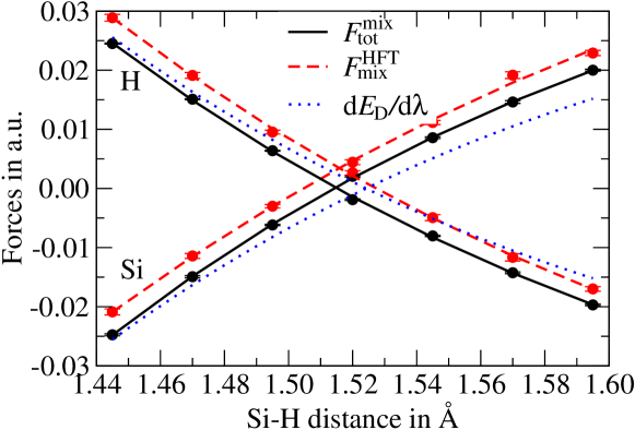
Figure 1: The mixed estimates of the Hellmann-Feynman force ($F_{\rm mix}^{\rm HFT}$) and the total force ($F_{\rm mix}^{\rm tot}$) evaluated for the H and Si atoms. The derivative of the Morse potential fitted to the DMC energies (${\rm d}E_{\rm D}/{\rm d}\lambda$) is shown as reference.

Results using the mixed distribution expression of equation (11) with the approximation of (12) are plotted in figure 1. As reference, we have also plotted the derivative of the Morse potential previously obtained from a fit to the DMC energies. The minimum in the DMC energy occurs at a bond length of 1.5242(6) Å. The forces on the H and Si atoms should be equal and opposite, and figure 1 shows that the total forces $F_{\rm mix}^{\rm tot}$ on the H and Si atoms sum almost to zero over the range of bond lengths shown, with an error corresponding to an error in the bond length of equal or less than 0.001 Å. However, the total force gives an equilibrium bond length which is about 0.010 Å too short. The Hellmann-Feynman force $F_{\rm mix}^{\rm HFT}$ on the H atom is zero at a bond length which is 0.003(1) Å too long, while that on the Si atom is zero at a bond length which is 0.020(1) Å too short. Including the Pulay terms improves the agreement between the forces calculated on the H and Si atoms, but overall the bond lengths from the mixed-estimator forces are no better than those which could be obtained in DFT calculations.

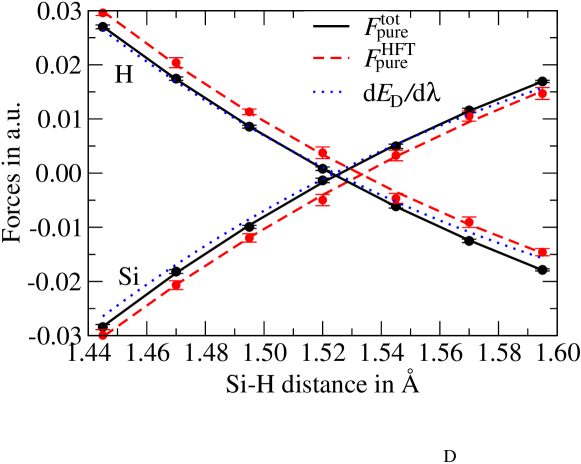
Figure 2: The same as figure 1, but for the pure forces evaluated using equation (21).

Results using equation (21) are plotted in figure 2. We refer to this as the expression for the pure forces, although it also contains a term evaluated with the variational distribution. The total pure forces $F_{\rm pure}^{\rm tot}$ on the H and Si atoms sum almost to zero over the range of bond lengths shown, with an error corresponding to an error in the bond length of less than 0.003 Å, which is about three times the statistical error. The equilibrium bond lengths from the zero force condition are also within statistical errors of the equilibrium bond length obtained from the minimum in the DMC energy. The nodal terms in equation (21) are by no means negligible. The pure Hellmann-Feynman forces $F_{\rm pure}^{\rm HFT}$ on the H and Si atoms do not sum to zero, and the force on the H atom is zero at a bond length which is 0.008(1) Å too long, while the force on the Si atom is zero at a bond length which is 0.010(2) Å too long. The total pure forces are much more accurate than the total mixed forces, which suggests that the approximate forms of equation (21) and ${\rm d}\Psi_{\rm T}/{\rm d}\lambda$ give rather accurate results in our simulations. The bond lengths obtained from the total forces and from the HFT term, and using forces on the Si and H atoms, within mixed and pure DMC, are summarised in Table 1. It is clear that the total pure forces give equilibrium bond lengths differing from that obtained from the DMC energies by much less than the typical error in DFT bond lengths of $\sim$0.01 Å.

Table 1: Equilibrium bond lengths $a$ in Å for the SiH molecule obtained from the total forces and from the HFT term and using forces on the Si and H atoms, within mixed and pure DMC. The equilibrium bond length obtained from the minimum in the DMC energy curve is 1.5242(6) Å.

	mixed DMC	pure DMC
$a^{\rm tot}$ (Si)	1.5140(3)	1.5259(8)
$a^{\rm HFT}$ (Si)	1.5044(8)	1.5343(16)
$a^{\rm tot}$ (H)	1.5150(3)	1.5227(7)
$a^{\rm HFT}$ (H)	1.5272(9)	1.5320(12)

7 Statistical properties of the force estimators

A statistical estimate of a quantity should be accompanied by a confidence interval which indicates the reliability of the estimate. Consider a probability distribution function (PDF) $P(x)$ which has a mean value $\mu$ and variance $\sigma^{2}$. The mean value of a random variable $x$ drawn from $P(x)$ may be estimated using the sample mean,

$$\bar{x}_{N}=\frac{1}{N}\sum_{i=1}^{N}x_{i}\;,$$ (23)

and the variance estimated using the sample variance,

$$\sigma_{N}^{2}=\frac{1}{N-1}\sum_{i=1}^{N}\left(x_{i}-\bar{x}_{N}\right)^{2}\;.$$ (24)

We then say that $\bar{x}_{N}$ lies within the interval $\left[\bar{x}_{N}-{\sigma_{N}}/\sqrt{N},\,\bar{x}_{N}+{\sigma_{N}}/\sqrt{N}\right]$ with a confidence of 68 %.

This statement relies upon the probability distribution satisfying certain conditions which are the content of the Law of Large Numbers (LLN) and the Central Limit Theorem (CLT). The LLN concerns the statistical convergence of the sum in equation (23) to the true mean value with increasing $N$. Similarly, the CLT concerns the statistical convergence with increasing $N$ of the probability distribution from which $\bar{x}_{N}$ is drawn to a Normal distribution with mean $\mu=\int xP(x)\,dx$ and variance $\sigma^{2}/N=1/N\int(x-\mu)^{2}P(x)\,dx$. For the LLN to be valid it is sufficient that the first moment of $P(x)$ exists, which requires that $P(x)$ decays faster than $|x-x_{0}|^{-2}$, where $x_{0}$ is a constant. Similarly, the CLT is valid if the second moment of $P(x)$ exists, which requires that $P(x)$ decays faster than $|x-x_{0}|^{-3}$.

Equations (5) and (8) show that the VMC and DMC energies are evaluated as averages of local energies $E_{\rm L}({\bf R}_{i})$. The probability distribution of the local energies $P(E_{\rm L})$ is generally non-Gaussian and has “fat tails”. The asymptotic behaviour of $P(E_{\rm L})$ is determined by the singularities in $E_{\rm L}$. Trail [49] considered singularities in $E_{\rm L}$ arising from a Coulomb energy divergence at particle coalescences, divergences in the local kinetic energy at the nodal surface of $\Psi_{\rm T}$, and in finite systems where $\Psi_{\rm T}$ has the wrong asymptotic behaviour. The Coulomb energy divergence at particle coalescences can be removed by imposing the Kato cusp conditions on $\Psi_{\rm T}$, as is normally done in QMC calculations, but it is not clear how to remove the divergences at the nodal surface. Trail [49] showed that the singularities in $E_{\rm L}$ lead to tails in $P(E_{\rm L})$ which decay as $|E_{\rm L}-E_{0}|^{-4}$, where $E_{0}$ is a constant. Consequently the energy estimate is drawn from a Normal distribution whose variance we may estimate (in the limit of large $N$). However, the estimated variance of the local energy is drawn from a distribution of infinite variance that is not Normal, hence it is not entirely clear how to obtain a meaningful confidence interval for this estimate.

A similar analysis can be performed for the forces. Each term in the force can be written as a sum of local contributions,

$$F\simeq\frac{1}{N}\sum_{i=1}^{N}F_{\rm L}({\bf R}_{i})\;.$$ (25)

For the Hellmann-Feynman term we distinguish between three cases: an all-electron atom, a smooth local pseudopotential, and a smooth non-local pseudopotential. The probability distribution of the Hellmann-Feynman term for an all-electron atom has slowly decaying tails of the form $|F_{\rm L}-F_{0}|^{-5/2}$, where $F_{0}$ is a constant. In this case the LLN applies but the CLT is not satisfied, and the variance of the Hellmann-Feynman force is infinite. Although a sample variance can be calculated it does not statistically converge to a constant value with increasing $N$, and it is not related to the width of the distribution from which the estimated force is drawn. The infinite variance in the Hellmann-Feynman force for an all-electron atom has long been recognised and methods for dealing with it have been devised. Assaraf and Caffarel [25, 27] suggested adding a term to the HFT force which has zero mean but may greatly reduce the sample variance. (This amounts to adding the term containing ${\rm d}\Psi_{\rm T}/{\rm d}\lambda$ in the first term on the right hand side of equations (10) and (21).) A similar approach was developed by Per et al [50]. Chiesa et al [51] developed a method to filter out the component of the electronic charge density responsible for the infinite variance. Using smooth local or non-local pseudopotentials without singularities at the nucleus also eliminates the infinite-variance problem arising from the electron-nucleus interaction. The terms in the force estimators which contain ${\rm d}\Psi_{\rm T}/{\rm d}\lambda$ also give probability distributions with $|F_{\rm L}-F_{0}|^{-5/2}$ tails, and hence the CLT is not applicable. The origin of the problem is that although $\Psi_{\rm T}$ is zero on the nodal surface, ${\rm d}\Psi_{\rm T}/{\rm d}\lambda$ is normally finite. Trail [52] and Attaccalite and Sorella [30] have devised rigorous methods within VMC to eliminate the infinite variance by altering the probability distribution near the nodes.

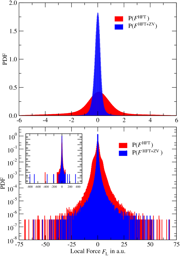
Figure 3: The probability distribution of the VMC local Hellmann-Feynman forces (red) and the local Hellmann-Feynman forces with the zero variance force (blue). The forces on the Ge atom of a GeH molecule are shown calculated using non-local pseudopotentials and a Slater-Jastrow wave function. The distributions were generated from 10⁷ samples. The upper and lower graphs show the same data on different scales.

Figure 3 shows probability distributions for VMC local forces on the Ge atom in a GeH molecule. The upper graph shows that the probability distribution for the sum of the local Hellmann-Feynman force (the term in equation (10) containing ${\rm d}\hat{H}/{\rm d}\lambda$) and the local zero-variance force (the term in equation (10) containing $\hat{H}$) is much more strongly peaked in the region of the mean value than the local Hellmann-Feynman force itself. This illustrates the operation of the zero-variance term. The lower graphs show the same data plotted on different scales. The inset graph shows a very wide scale of local forces, and the local zero-variance force actually has more outlying contributions than the local Hellmann-Feynman force. This illustrates the result that the probability distribution of the local Hellmann-Feynman force has $|F_{\rm L}-F_{0}|^{-4}$ tails (for a smooth pseudopotential) and the CLT holds, while the probability distribution of the local zero-variance force has $|F_{\rm L}-F_{0}|^{-5/2}$ tails so that the CLT is not satisfied. This seems somewhat counterintuitive; without the zero-variance term the variance is finite but does not approach zero when $(\Psi_{\rm T},{\rm d}\Psi_{\rm T}/{\rm d}\lambda)$ are exact whereas, if we include the zero-variance term, the variance is zero for the exact case, but infinite for the approximate case. Analogous results apply for the DMC forces obtained with the mixed and pure distributions.

Currently no rigorous procedure has been demonstrated for removing the infinite variance which arises in DMC calculations of the Pulay forces. Although this state of affairs is unsatisfactory, the probability distribution of the local forces is strongly peaked in the region of the true value, which suggests that reasonable procedures for estimating a confidence interval can be devised.

8 Conclusions

We have formulated DMC forces evaluated with the pure distribution. The force can be written as the sum of a Hellmann-Feynman force and a term which can be cast as an integral over the nodal surface. The nodal term can be recast as an average over the pure distribution of a quantity which depends only on $\Psi_{\rm T}$ and ${\rm d}\Psi_{\rm T}/{\rm d}\lambda$. It is obvious that such an exact expression must exist, as $\Psi_{\rm T}$ and ${\rm d}\Psi_{\rm T}/{\rm d}\lambda$ fix both the nodal surface and its first order variation, which in turn fix the DMC energy and its first derivative. It is however, very awkward to evaluate an integral over the nodal surface, and therefore we have adopted an approximate approach to evaluating it which has an error of order $(\Psi_{\rm T}-\Phi)^{2}$. Our final expression (21) consists of integrals over the pure and variational distributions, both of which exhibit a zero variance property.

The forces evaluated using equation (21) yield bond lengths for the SiH molecule with an error (with respect to DMC energy calculations) of much less than 0.01 Å, which is acceptable for most purposes. Of course, before claiming that the problem of calculating DMC forces is “solved”, accurate results for heavier atoms and larger systems are required. To this we should add the issues of efficient generation of the pure probability distribution for large systems, overcoming the “infinite variance” described in Section 7, obtaining accurate forms for $\Psi_{\rm T}$ and ${\rm d}\Psi_{\rm T}/{\rm d}\lambda$, and (hopefully) removing the second approximation in equation (21). Notwithstanding these caveats, we believe that substantial progress has been made in calculating DMC forces, and that their evaluation will become routine in the not-too-distant future.

9 Acknowledgments

This work has been supported by the Engineering and Physical Sciences Research Council (EPSRC), UK. PDH was supported by a Royal Society University Research Fellowship. Computing resources were provided by the Cambridge High Performance Computing Service.

References

References

- [1] Foulkes W M C, Mitáš L, Rajagopal G and Needs R J 2001 Rev. Mod. Phys. 73 33
- [2] Ceperley D M and Alder B J 1980 Phys. Rev. Lett. 45 566
- [3] Drummond N D, Radnai Z, Trail J R, Towler M D and Needs R J 2004 Phys. Rev. B 69 085116
- [4] Drummond N D and Needs R J 2009 Phys. Rev. Lett. 102, 126402
- [5] Williamson A J, Grossman J C, Hood R Q, Puzder A and Galli G 2002 Phys. Rev. Lett. 89 196803
- [6] Drummond N D, Williamson A J, Needs R J and Galli G 2005 Phys. Rev. Lett. 95 096801
- [7] Filippi C, Healy S B, Kratzer P, Pehlke E and Scheffler M 2002 Phys. Rev. Lett. 89 166102
- [8] Pozzo M and Alfè D 2008 Phys. Rev. B 78 245313
- [9] Leung W-K, Needs R J, Rajagopal G, Itoh S and Ihara S 1999 Phys. Rev. Lett. 83 2351
- [10] Hood R Q, Kent P R C, Needs R J and Briddon P R 2003 Phys. Rev. Lett. 91 076403
- [11] Alfè D and Gillan M J 2005 Phys. Rev. B 71 220101
- [12] Alfè D, Alfredsson M, Brodholt J, Gillan M J, Towler M D and Needs R J 2005 Phys. Rev. B 72 014114
- [13] Natoli V, Martin R M and Ceperley D M 1993 Phys. Rev. Lett. 70 1952
- [14] Delaney K T, Pierleoni C and Ceperley D M 2006 Phys. Rev. Lett. 97 235702
- [15] Maezono R, Ma A, Towler M D and Needs R J 2007 Phys. Rev. Lett. 98 025701
- [16] Pozzo M and Alfè D 2008 Phys. Rev. B 77 104103
- [17] Needs R J, Towler M D, Drummond N D and López Ríos P CASINO version 2.2 User Manual, University of Cambridge, Cambridge 2008
- [18] Ceperley D M and Kalos M H in Monte Carlo Methods in Statistical Physics, edited by Binder K (Springer, Berlin, 1979), pp 145–194
- [19] Filippi C and Umrigar C J 2000 Phys. Rev. B 61 16291
- [20] Pierleoni C and Ceperley D M 2005 Chem. Phys. Chem. 6 1872
- [21] Anderson J B 1975 J. Chem. Phys. 63 1499
- [22] Anderson J B 1976 J. Chem. Phys. 65 4121
- [23] Barnett R N, Reynolds P J and Lester, W A Jr 1991 J. Comput. Phys. 96 258
- [24] Baroni S and Moroni S 1999 Phys. Rev. Lett. 82 4745
- [25] Assaraf R and Caffarel M 1999 Phys. Rev. Lett. 83 4682
- [26] Casalegno M, Mella M and Rappe A M 2003 J. Chem. Phys. 118 7193
- [27] Assaraf R and Caffarel M 2003 J. Chem. Phys. 119 10536
- [28] Lee M W, Mella M and Rappe A M 2005 J. Chem. Phys. 122 244103
- [29] Badinski A and Needs R J 2007 Phys. Rev. E 76 036707
- [30] Attaccalite C and Sorella S 2008 Phys. Rev. Lett. 100 114501
- [31] Badinski A and Needs R J 2008 J. Chem. Phys. 129 224101
- [32] Reynolds P J, Barnett R N, Hammond B L, Grimes R M and Lester W A Jr 1986 Int. J. Quant. Chem. 29 589
- [33] Huang K C, Needs R J and Rajagopal G 2000 J. Chem. Phys. 112 4419
- [34] Schautz F and Flad H-J 2000 J. Chem. Phys. 112 4421
- [35] Badinski A, Haynes P D and Needs R J 2008 Phys. Rev. B 77 085111
- [36] Takada M, Dupuis M, and King H F 1983 J. Comput. Chem. 4, 234
- [37] Trail J R and Needs R J 2005 J. Chem. Phys. 122 014112
- [38] Trail J R and Needs R J 2005 J. Chem. Phys. 122 174109
- [39]
- [40] Mitáš L, Shirey E L and Ceperley D M 1991 J. Chem. Phys. 95 3467
- [41] Badinski A and Needs R J 2008 Phys. Rev. B 78, 035134
- [42] Schmidt M W, Baldridge K K and Boatz J A 1993 J. Comput. Chem. 14 1347
- [43] Drummond N D, Towler M D and Needs R J 2004 Phys. Rev. B 70 235119
- [44] Drummond N D and Needs R J 2005 Phys. Rev. B 72 085124
- [45] Umrigar C J, Toulouse J, Filippi C, Sorella S and Hennig R G 2007 Phys. Rev. Lett. 98 110201
- [46] Toulouse J and Umrigar C J 2007 J. Chem. Phys. 126 084102
- [47] Brown M D, Trail J R, López Ríos P and Needs R J 2007 J. Chem. Phys. 126 224110
- [48] López Ríos P, Ma A, Drummond N D, Towler M D and Needs R J 2006 Phys. Rev. E 74 066701
- [49] Trail J R 2008 Phys. Rev. E 77 016703
- [50] Per M C, Russo S P and Snook I K 2008 J. Chem. Phys. 128 114106
- [51] Chiesa S, Ceperley D M and Zhang S 2005 Phys. Rev. Lett. 94 036404
- [52] Trail J R 2008 Phys. Rev. E 77 016704