A generalized Kramers-Kronig transform for Casimir effect computations

Abstract

Recent advances in experimental techniques now permit to measure the Casimir force with unprecedented precision. In order to achieve a comparable precision in the theoretical prediction of the force, it is necessary to accurately determine the electric permittivity of the materials constituting the plates along the imaginary frequency axis. The latter quantity is not directly accessible to experiments, but it can be determined via dispersion relations from experimental optical data. In the experimentally important case of conductors, however, a serious drawback of the standard dispersion relations commonly used for this purpose, is their strong dependence on the chosen low-frequency extrapolation of the experimental optical data, which introduces a significant and not easily controllable uncertainty in the result. In this paper we show that a simple modification of the standard dispersion relations, involving suitable analytic window functions, resolves this difficulty, making it possible to reliably determine the electric permittivity at imaginary frequencies solely using experimental optical data in the frequency interval where they are available, without any need of uncontrolled data extrapolations.

I INTRODUCTION

One of the most intriguing predictions of Quantum electrodynamics is the existence of irreducible vacuum fluctuations of the electromagnetic (e.m.) field. It was Casimir’s fundamental discovery casimir to realize that this purely quantum phenomenon was not confined to the atomic scale, as in the Lamb shift, but would rather manifest itself also at the macroscopic scale, in the form of a force of attraction between two discharged plates. For the idealized case of two perfectly reflecting plane-parallel plates at zero temperature, placed at a distance $a$ in vacuum, Casimir obtained the following remarkably simple estimate of the force per unit area

$$F_{C}=\frac{\pi^{2}\hbar c}{240\;a^{4}}\;.$$ (1)

An important step forward was made a few years later by Lifshitz and co-workers lifs , who obtained a formula for the force between two homogeneous dielectric plane-parallel slabs, at finite temperature. In this theory, of macroscopic character, the material properties of the slabs were fully characterized in terms of the respective frequency dependent electric permittivities $\epsilon(\omega)$, accounting for the dispersive and dissipative properties of real materials. In this way, it was possible for the first time to investigate the influence of material properties on the magnitude of the Casimir force.

Over ten years ago, a series of brilliant experiments lamor ; roy exploiting modern experimental techniques provided the definitive demonstration of the Casimir effect. These now historical experiments spurred enormous interest in the Casimir effect, and were soon followed by many other experiments. The subsequent experiments were aimed at diverse objectives. Some of them explored new geometries: while the works lamor ; roy used a sphere-plate setup, the original planar geometry investigated by Casimir was adopted in the experiment Bressi , and a setup with crossed cylinders was considered in ederth . The important issue of the non trivial geometry dependence of the Casimir effect is also being pursued experimentally, using elaborate micro-patterned surfaces Bao . Other experiments aimed at demonstrating new possible uses of the Casimir force, like for example the actuation of micromachines capasso , or at demonstrating the possibility of a large modulation of the Casimir force chen ; iannuzzi , which could also result in interesting technological applications. There are also experiments using superconducting Casimir cavities, that aim at measuring the change of the Casimir energy across the superconducting phase transition bimonte . The experiments performed in the last ten years are just too numerous to mention them all here. For an updated account we refer the reader to the very recent review paper Mohid .

Apart from exploring new manifestations of the Casimir effect, a large experimental effort is presently being made also to increase the precision of Casimir force measurements, in simple geometries. Already in the early experiment roy a precision upto one percent was obtained. More recently, a series of experiments with microtorsional oscillators decca reached an amazing precision of 0.2 percent. The reader may wonder what is the interest in achieving such a high precision in this kind of experiments. There are several reasons why this is important. On one hand, in the theory of dispersion forces puzzling conceptual problems have recently emerged that are connected with the contribution of free charges to the thermal Casimir force, whose resolution crucially depends on the precision of the theory-experiment comparison Mohid . On the other hand, the ability to accurately determine the Casimir force is also important for the purpose of obtaining stronger constraints on hypothetical long-range forces predicted by certain theoretical scenarios going beyond the Standard Model of particle physics Mohid .

The remarkable precision achieved in the most recent experiments poses a challenging demand on the theorist: is it possible to predict the magnitude of the Casimir force with a comparable level of precision, say of one percent? Assessing the theoretical error affecting present estimates of the Casimir force is a difficult problem indeed, because many different factors must be taken into account Mohid . Consider the typical experimental setting of most of the current experiments, where the Casimir force is measured between two bodies covered with gold, placed in vacuum at a distance of a (few) hundred nanometers. In this separation range, the main factor to consider is the finite penetration depth of electromagnetic fields into the gold layer , resulting from the finite conductivity of gold. The tool to analyze the influence of such material properties as the conductivity on the Casimir effect is provided by Lifshitz theory lifs . This theory shows that for a separation of 100 nm, the finite conductivity of gold determines a reduction in the magnitude of the Casimir force of about fifty percent in comparison with the perfect metal result lambr . Much smaller corrections, that must nevertheless be considered if the force is to be estimated with percent precision, arise from the finite temperature of the plates and from their surface roughness. Moreover, geometric effects resulting from the actual shape of the plates should be considered. We should also mention that the magnitude of residual electrostatic forces between the plates, resulting from contact potentials and patch effects, must be carefully accounted for. For a discussion of all these issues, which received much attention in the recent literature on the Casimir effect, we again address the reader to Ref. Mohid . See also the recent work rudy .

In this paper, we focus our attention on the influence of the optical properties of the plates which, as explained above, is by far the most relevant factor to consider. As we pointed out earlier, in Lifshitz theory the optical properties of the plates enter via the frequency-dependent electric permittivity $\epsilon(\omega)$ of the material constituting plates. In order to obtain an accurate prediction of the force, it is therefore of the utmost importance to use accurate data for the electric permittivity. The common practice adopted in all recent Casimir experiments with gold surfaces is to use tabulated data for gold (most of the times those quoted in Refs. palik ), suitably extrapolated at low frequencies, where optical data are not available, by simple analytic models (like the Drude model or the so-called generalized plasma model). However, already ten years ago Lamoreaux observed lamor2 that using tabulated data to obtain an accurate prediction of the Casimir force may not be a reliable practice, since optical properties of gold films may vary significantly from sample to sample, depending on the conditions of deposition. The same author stressed the importance of measuring the optical data of the films actually used in the force measurements, in the frequency range that is relevant for the Casimir force. The importance of this point was further stressed in Piro and received clear experimental support in a recent paper sveto , where the optical properties of several gold films of different thicknesses, and prepared by different procedures, were measured ellipsometrically in a wide range of wavelengths, from 0.14 to 33 microns, and it was found that the frequency dependent electric permittivity changes significantly from sample to sample. By using the zero-temperature Lifshitz formula, the authors estimated that the observed sample dependence of the electric permittivity implies a variation in the theoretical value of the Casimir force, from one sample to another, easily as large as ten percent, for separations around 100 nm. It was concluded that in order to achieve a theoretical accuracy better than ten percent in the prediction of the Casimir force, it is necessary to determine the optical properties of the films actually used in the experiment of interest.

The aim of this paper is to improve the mathematical procedure that is actually needed to obtain reliable estimates of the Casimir force, starting from experimental optical data on the material of the plates, like those presented in Ref. sveto . The necessity of such an improvement stems from the very simple and unavoidable fact that experimental optical data are never available in the entire frequency domain, but are always restricted to a finite frequency interval $\omega_{\rm min}<\omega<\omega_{\rm max}$. To see why this constitutes problem we recall that Lifshitz formula, routinely used to interpret current experiments, expresses the Casimir force between two parallel plates as an integral over imaginary frequencies ${\rm i}\xi$ of a quantity involving the dielectric permittivities of the plates $\epsilon({\rm i\xi})$. For finite temperature, the continuous frequency integration is replaced by a sum over discrete so-called Matsubara frequencies $\omega_{n}={\rm i}\xi_{n}$, where $\xi_{n}=2\pi nk_{B}T/\hbar$, with $n$ a non-negative integer, and $T$ the temperature of the plates. In any case, whatever the temperature, one needs to evaluate the permittivity of the plates for certain imaginary frequencies. We note that, in principle, recourse to imaginary frequencies is not mandatory because it is possible to rewrite Lifshitz formula in a mathematically equivalent form, involving an integral over the real frequency axis. In this case however the integrand becomes a rapidly oscillating function of the frequency, which hampers any possibility of numerical evaluation. In practice, the real-frequency form of Lifshitz formula is never used, and only its imaginary-frequency version is considered. We remark that occurrence of imaginary frequencies in the expression of the Casimir force, is a general feature of all recent formalisms, extending Lifshitz theory to non-planar geometries emig ; kenneth ; lambr2 . The problem is that the electric permittivity $\epsilon(i\xi)$ at imaginary frequencies cannot be measured directly by any experiment. The only way to determine it by means of dispersion relations, which allow to express $\epsilon(i\xi)$ in terms of the observable real-frequency electric permittivity $\epsilon(\omega)$. In the standard version of dispersion relations lifs , adopted so far in all works on the Casimir effect, $\epsilon({\rm i}\xi)-1$ is expressed in terms of an integral of a quantity involving the imaginary part $\epsilon^{\prime\prime}(\omega)$ of the electric permittivity:

$$\epsilon({\rm i}\xi)-1=\frac{2}{\pi}\int_{0}^{\infty}d\omega\frac{\omega\,\epsilon^{\prime\prime}(\omega)}{\omega^{2}+\xi^{2}}\;.$$ (2)

The above formula shows that, in principle, a determination of $\epsilon({\rm i}\xi)$ requires knowledge of $\epsilon^{\prime\prime}(\omega)$ at all frequencies while, as we said earlier, optical data are available only in some interval $\omega_{\rm min}<\omega<\omega_{\rm max}$. In practice, the problem is not so serious on the high frequency side, because the fall-off properties of $\epsilon^{\prime\prime}(\omega)$ at high frequencies, together with the $\omega^{2}$ factor in the denominator of the integrand, ensure that the error made by truncating the integral at a suitably large frequency $\omega_{\rm max}$ is small, provided that $\omega_{\rm max}$ is large enough. Typically, an $\omega_{\rm max}$ larger than, say, $15c/(2a)$, is good enough for practical purposes. Things are not so easy though on the low frequency side. In the case of insulators, optical data are typically available until frequencies $\omega_{\min}$ much smaller than the frequencies of all resonances of the medium. Because of this, $\epsilon^{\prime\prime}(\omega)$ is almost zero for $\omega<\omega_{\rm min}$, and therefore the error made by truncating the integral at $\omega_{\rm min}$ is again negligible. Problems arise however in the case of ohmic conductors, because then $\epsilon^{\prime\prime}(\omega)$ has a $1/\omega$ singularity at $\omega=0$. As a result $\epsilon^{\prime\prime}(\omega)$ becomes extremely large at low frequencies, in such a way that the integral in Eq. (2) receives a very large contribution from low frequencies. For typical values of $\omega_{\rm min}$ that can be reached in practice (for example for gold, the tabulated data in palik begin at $\omega_{\rm min}=125$ meV$/\hbar$, while the data of sveto start at 38 meV$/\hbar$) truncation of the integral at $\omega_{\rm min}$ results in a large error. The traditional remedy to this problem is to make some analytical extrapolation of the data, typically based on Drude model fits of the low-frequency region of data, from $\omega_{\rm min}$ to zero, and then use the extrapolation to estimate the contribution of the integral in the interval $0<\omega<\omega_{\rm min}$ where data are not directly available. It is important to observe that this contribution is usually very large. For example, even in the case of Ref. sveto , the relative contribution of the extrapolation is about fifty percent of the total value of the integral, in the entire range of imaginary frequencies that are needed for estimating the Casimir force.

Clearly, this procedure is not very satisfying. The use of analytical extrapolations of the data introduces an uncertainty in the obtained values of $\epsilon({\rm i}\xi)$, that is not easy to quantify. The result may in fact depend a lot on the form of the extrapolation, and there is no guarantee that the chosen expression is good enough. Consider for example Ref. sveto , which constitutes the most accurate existing work on this problem. It was found there that the simple Drude model does not fit so well the data of all samples, making it necessary to improve it by the inclusion of an additional Lorentz oscillator. Moreover, it was found that for each sample the Drude parameters extracted from the data depended on the used fitting procedure, and were inconsistent which each other within the estimated errors, which is again an indication of the probable inadequacy of the analytical expression chosen for the interpolation. This state of things led us to investigate if it possible to determine accurately $\epsilon({\rm i\xi})$ solely on the basis of available optical data, without making recourse to data extrapolations. We shall see below that this is indeed possible, provided that Eq. (2) is suitably modified, in a way that involves multiplying the integrand by an appropriate analytical window function $f(\omega)$, which suppresses the contribution of frequencies not belonging to the interval $\omega_{\rm min}<\omega<\omega_{\rm max}$. As a result of this modification, the error made by truncating the integral to the frequency range $\omega_{\rm min}<\omega<\omega_{\rm max}$ can be made negligible at both ends of the integration domain, rendering unnecessary any extrapolation of the optical data outside the interval where they are available. The procedure outlined in this paper should allow to better evaluate the theoretical uncertainty of Casimir force estimates resulting from experimental errors in the optical data.

The plan of the paper is as follows: in Sec. II we derive a generalized dispersion relation for $\epsilon({\rm i}\xi)$, involving analytic window functions $f(z)$, and we provide a simple choice for the window functions. In Sec III we present the results of a numerical simulation of our window functions, for the experimentally relevant case of gold, and in Sec IV we estimate numerically the error on the Casimir pressure resulting from the use of our window functions. Sec V contains our conclusions and a discussion of the results.

II Generalized dispersion relations with window-functions

As it it well known lifs , analyticity properties satisfied by the electric permittivity $\epsilon(\omega)$ of any causal medium (and more in general by any causal response function, the magnetic permeability $\mu(\omega)$ being another example) imply certain integral relations between the real part $\epsilon^{\prime}(\omega)$ and imaginary part $\epsilon^{\prime\prime}(\omega)$ of $\epsilon(\omega)$, known as Kramers-Kronig or dispersion relations. The dispersion relation of interest to us is the one that permits to express the value $\epsilon({\rm i}\xi)$ of the response function at some imaginary frequency ${\rm i}\xi$ in terms of an integral along the positive frequency axis, involving $\epsilon^{\prime\prime}(\omega)$. It is convenient to briefly review here the simple derivation of this important result, which is an easy exercise in contour integration. For our purposes, it is more convenient to start from an arbitrary complex function $u(z)$, with the following properties: $u(z)$ is analytic in the upper complex plane ${\cal C}^{+}=\{z:{\rm Im}(z)>0\}$, fall’s off to zero for large $|z|$ like some power of $|z|$, and admits at most a simple pole at $\omega=0$. Consider now the closed integration contour $\Gamma$ obtained by closing in the upper complex plane the positively oriented real axis, and let $z_{0}$ be any complex number in ${\cal C}^{+}$. It is then a simple matter to verify the identity:

$$\int_{\Gamma}dz\frac{z\,u(z)}{z^{2}-z_{0}^{2}}={\rm i}\pi u(z_{0})\;.$$ (3)

The assumed fall-off property of $u(z)$ ensures that the half-circle of infinite radius forming $\Gamma$ contributes nothing to the integral, and then from Eq. (3) we find:

$$u(z_{0})=\frac{1}{{\rm i}\pi}\int_{-\infty}^{\infty}d\omega\frac{\omega\,u(\omega)}{\omega^{2}-z_{0}^{2}}\;.$$ (4)

Consider now a purely imaginary complex number $z_{0}={\rm i}\xi$, and assume in addition that along the real axis $u(\omega)$ satisfies the symmetry property $u(-\omega)=u^{*}(\omega)$. From Eq. (4) we then find:

$$u({\rm i}\xi)=\frac{2}{\pi}\int_{0}^{\infty}d\omega\frac{\omega\,u^{\prime\prime}(\omega)}{\omega^{2}+\xi^{2}}\;,$$ (5)

which is the desired result.

The standard dispersion relation Eq. (2) used to compute the electric permittivity for imaginary frequencies is a special case of the above relation, corresponding to choosing $u(z)=\epsilon(z)-1$. We note that Eq. (2) is valid both for insulators, which have a finite permittivity at zero frequency, as well as for ohmic conductors, whose permittivity has a $1/\omega$ singularity in the origin. As we explained in the introduction Eq. (2), even though perfectly correct from a mathematical standpoint, has serious drawbacks, when it is used to numerically estimate $\epsilon(i\xi)$ for ohmic conductors, starting from optical data available only in some interval $\omega_{\rm min}<\omega<\omega_{\rm max}$, because the integral on the r.h.s. of Eq. (2) receives a large contribution from frequencies near zero, where data are not available. This difficulty can however be overcome in a very simple way, as we now explain. Consider a window function $f(z)$, enjoying the following properties: $f(z)$ is analytic in ${\cal C}^{+}$, it has no poles in ${\cal C}^{+}$ except possibly a simple pole at infinity, and satisfies the symmetry property

$$f(-z^{*})=f^{*}(z)\;.$$ (6)

Consider now Eq. (5), for $u(z)=f(z)(\epsilon(z)-1)$. Since for any medium $(\epsilon(z)-1)$ falls off like $z^{-2}$ at infinity lifs2 , the quantity $u(z)$ falls off at least like $z^{-1}$ at infinity, and it satisfies all the properties required for Eq. (5) to hold. For any $\xi$ such that $f(i\xi)\neq 0$, we then obtain the following generalized dispersion relation:

$$\epsilon({\rm i}\xi)-1=\frac{2}{\pi\,f({\rm i}\xi)}\int_{0}^{\infty}d\omega\frac{\omega\,}{\omega^{2}+\xi^{2}}{\rm Im}[f(\omega)(\epsilon(\omega)-1)]\;.$$ (7)

We note that the above relation constitutes an exact result, generalizing the standard dispersion relation Eq. (2), to which it reduces with the choice $f(z)=1$. Another form of dispersion relation, frequently used in the case of conductors or superconductors bimonte ; bimonte2 is obtained by taking $f(z)={\rm i}\,z$ into Eq. (7). Recalling the relation lifs2

$$\epsilon(\omega)=1+\frac{4\pi i}{\omega}\,\sigma(\omega)\;,$$ (8)

it reads:

$$\epsilon({\rm i}\xi)-1=\frac{8}{\xi}\int_{0}^{\infty}d\omega\frac{\omega\,}{\omega^{2}+\xi^{2}}{\rm Im}\,[\sigma(\omega)]\;.$$ (9)

The above form is especially convenient in the case of superconductors, because it avoids the $\delta(\omega)$ singularity characterizing the real part of the conductivity of these materials bimonte2 .

We observe now, and this is the key point, that there is no reason to restrict the choice of the function $f(z)$ to these two possibilities. Indeed, we can take advantage of the freedom in the choice of $f(z)$, to suppress the unwanted contribution of low frequencies (as well as of high frequencies), where experimental data on $\epsilon(\omega)$ are not available. In order to do that, it is sufficient to choose a window function that goes to zero fast enough for $\omega\rightarrow 0$, as well as for $\omega\rightarrow\infty$. A convenient family of window functions which do the job is the following:

$$f(z)=A\,z^{2p+1}\left[\frac{1}{(z-w)^{2q+1}}+\frac{1}{(z+w^{*})^{2q+1}}\right]\;,$$ (10)

where $w$ is an arbitrary complex number such that ${\rm Im}(w)<0$, and $p$ and $q$ are integers such that $p<q$. The constant $A$ is an irrelevant arbitrary normalization constant, that drops out from the generalized dispersion formula Eq. (7). As we see, in the limit $z\rightarrow 0$, these functions vanish like $z^{2p+1}$, and therefore by taking sufficiently large values for $p$ we can obtain suppression of low frequencies to any desired level. On the other hand, for $z\rightarrow\infty$, $f(z)$ vanishes like $z^{2(p-q)}$, and therefore by taking sufficiently large values of $q$, we can obtain suppression of high frequencies. Moreover, by suitably choosing the free parameter $w$, we can also adjust the range of frequencies that effectively contribute to the integral on the r.h.s. of Eq. (7). In Figs. 1 and 2 we plot the real and imaginary parts (in arbitrary units) of our window functions $f(\omega)$, versus the frequency $\omega$ (expressed in eV). The two curves displayed correspond to the choices $p=1,\,q=2$ (dashed line) and $p=1,\,q=3$ (solid line). In both cases, the parameter $w$ has the value $w=(1-2\,{\rm i})\,{\rm eV}/\hbar$.

Figure 1: Real part $f^{\prime}(\omega)$ (in arbitrary units) of the window functions in Eq. (10) versus frequency $\omega$ (in eV/$\hbar$). The window parameters are $p=1,\,q=2$ (dashed line), $p=1,\,q=3$ (solid line). In both cases, the parameter $w$ has the value $w=(1-2\,{\rm i})\,{\rm eV}/\hbar$.

Figure 2: Imaginary part $f^{\prime\prime}(\omega)$ (in arbitrary units) of the window functions in Eq. (10) versus frequency $\omega$ (in eV/$\hbar$). The window parameters are $p=1,\,q=2$ (dashed line), $p=1,\,q=3$ (solid line). In both cases, the parameter $w$ has the value $w=(1-2\,{\rm i})\,{\rm eV}/\hbar$.

Figure 3: Plots (in arbitrary units) of the window functions $f({\rm i}\xi)$ in Eq. (10) versus the imaginary frequency $\xi$ (in eV/$\hbar$). The window parameters are $p=1,\,q=2$ (dashed line), $p=1,\,q=3$ (solid line). In both cases, the parameter $w$ has the $w=(1-2\,{\rm i})\,{\rm eV}/\hbar$.

We observe that along the real frequency axis, our window functions have non-vanishing real and imaginary parts. This is not a feature of our particular choice of the window functions, but it is an unavoidable consequence of our demand of analyticity on $f(z)$. Indeed, for real frequencies $\omega$ the real and imaginary parts of $f(\omega)$ are related to each other by the usual Kramers-Kronig relations lifs that hold for the boundary values of analytic functions. In the case when $f(z)$ vanishes at infinity, they read:

$$f^{\prime}(\omega)=\frac{1}{\pi}{\rm P}\int_{-\infty}^{\infty}d\xi\,\frac{f^{\prime\prime}(\xi)}{\xi-\omega}\;,$$ (11)

$$f^{\prime\prime}(\omega)=-\frac{1}{\pi}{\rm P}\int_{-\infty}^{\infty}d\xi\,\frac{f^{\prime}(\xi)}{\xi-\omega}\;,$$ (12)

where the symbol ${\rm P}$ in front of the integrals denotes the principal value. These relation show that vanishing of $f^{\prime}(\omega)$ implies that of $f^{\prime\prime}(\omega)$ and viceversa, and therefore neither $f^{\prime}(\omega)$ nor $f^{\prime\prime}(\omega)$ can be identically zero. By virtue of this property of the window functions, it follows from Eq. (7) that both the real and imaginary parts of $\epsilon(\omega)$ are needed to evaluate $\epsilon({\rm i}\xi)$ (unless the standard choices $f(z)\equiv 1$ or $f(z)={\rm i}\,z$ are made). We also note (see Fig. 1 and 2) that the real and imaginary parts of $f(\omega)$ do not have a definite sign. This feature also is a general consequence of our key demand that $f(z)$ vanishes in the origin, as it can be seen by taking $\omega=0$ in Eqs. (11) and (12). Since the l.h.s. of both equations are required to vanish, the integrand on the r.h.s. cannot have a definite sign. Finally, in Fig 3 we show plots of two of our window functions $f({\rm i}\xi)$, versus the imaginary frequency $\xi$, expressed in eV, for the same two choices of parameters of Fig. 1 and 2. It is important to observe that the window functions $f(z)$ are real along the imaginary axis (as it must be, as a consequence of the symmetry property Eq. (6)). However, the sign of $f({\rm i}\xi)$ is not definite, and as a result of this $f({\rm i}\xi)$ admits zeros along the imaginary axis. When using Eq. (7) for estimating $\epsilon({\rm i\xi})$ it is then important to choose the window function such that none of its zeroes coincides with the value of $\xi$ for which $\epsilon({\rm i\xi})$ is being estimated.

III A numerical simulation

In this Section, we perform a simple simulation to test the degree of accuracy with which the quantity $\epsilon({\rm i}\xi)$ can be reconstructed using our window functions, starting from data on $\epsilon(\omega)$ referring to a finite frequency interval. To do that we can proceed as follows.

According to the standard dispersion relation Eq. (2), the quantity $\epsilon({\rm i}\xi)-1$ is equal to the integral on the r.h.s. of Eq. (2). Following Refs. Piro ; sveto , we can split this integral into three pieces, as follows:

$$\frac{2}{\pi}\int_{0}^{\infty}d\omega\frac{\omega\,\epsilon^{\prime\prime}(\omega)}{\omega^{2}+\xi^{2}}=I_{\rm low}(\xi)+I_{\rm exp}(\xi)+I_{\rm high}(\xi)\;,$$ (13)

where we set:

$$I_{\rm low}(\xi)=\frac{2}{\pi}\int_{0}^{\omega_{\rm min}}d\omega\frac{\omega\,\epsilon^{\prime\prime}(\omega)}{\omega^{2}+\xi^{2}}\;,$$ (14)

$$I_{\rm exp}(\xi)=\frac{2}{\pi}\int_{\omega_{\rm min}}^{\omega_{\rm max}}d\omega\frac{\omega\,\epsilon^{\prime\prime}(\omega)}{\omega^{2}+\xi^{2}}\;,$$ (15)

and

$$I_{\rm high}(\xi)=\frac{2}{\pi}\int_{\omega_{\rm max}}^{\infty}d\omega\frac{\omega\,\epsilon^{\prime\prime}(\omega)}{\omega^{2}+\xi^{2}}\;.$$ (16)

By construction, we obviously have:

$$\epsilon({\rm i}\xi)-1=I_{\rm low}(\xi)+I_{\rm exp}(\xi)+I_{\rm high}(\xi)\;.$$ (17)

An analogous split can be performed in the integral on the r.h.s. of the other standard dispersion relation involving the conductivity Eq. (9):

$$\frac{8}{\xi}\int_{0}^{\infty}d\omega\frac{\omega\,}{\omega^{2}+\xi^{2}}{\rm Im}\,[\sigma(\omega)]=K_{\rm low}(\xi)+K_{\rm exp}(\xi)+K_{\rm high}(\xi)\;,$$ (18)

with an obvious meaning of the symbols. Again, we have the identity:

$$\epsilon({\rm i}\xi)-1=K_{\rm low}(\xi)+K_{\rm exp}(\xi)+K_{\rm high}(\xi)\;.$$ (19)

On the other hand, according to our generalized dispersion relation Eq. (7), the quantity $\epsilon({\rm i}\xi)-1$ is also equal to the integral on the r.h.s. of Eq. (7). We can split this integral too in a way analogous to Eq. (13):

$$\frac{2}{\pi\,f({\rm i}\xi)}\int_{0}^{\infty}d\omega\frac{\omega\,}{\omega^{2}+\xi^{2}}{\rm Im}[f(\omega)(\epsilon(\omega)-1)]$$

$$=J_{\rm low}^{(p,q)}(\xi)+J_{\rm exp}^{(p,q)}(\xi)+J_{\rm high}^{(p,q)}(\xi)\;,$$ (20)

where we set:

$$J_{\rm low}^{(p,q)}(\xi)=\frac{2}{\pi\,f({\rm i}\xi)}\int_{0}^{\omega_{\rm min}}d\omega\frac{\omega\,}{\omega^{2}+\xi^{2}}{\rm Im}[f(\omega)(\epsilon(\omega)-1)]\;,$$ (21)

$$J_{\rm exp}^{(p,q)}(\xi)=\frac{2}{\pi\,f({\rm i}\xi)}\int_{\omega_{\rm min}}^{\omega_{\rm max}}d\omega\frac{\omega\,}{\omega^{2}+\xi^{2}}{\rm Im}[f(\omega)(\epsilon(\omega)-1)]\;,$$ (22)

and

$$J_{\rm high}^{(p,q)}(\xi)=\frac{2}{\pi\,f({\rm i}\xi)}\int_{\omega_{\rm max}}^{\infty}d\omega\frac{\omega\,}{\omega^{2}+\xi^{2}}{\rm Im}[f(\omega)(\epsilon(\omega)-1)]\;.$$ (23)

Then by construction we also have:

$$\epsilon({\rm i}\xi)-1=J_{\rm low}^{(p,q)}(\xi)+J_{\rm exp}^{(p,q)}(\xi)+J_{\rm high}^{(p,q)}(\xi)\;.$$ (24)

The quantities $I_{\rm exp}(\xi)$, $K_{\rm exp}(\xi)$ and $J_{\rm exp}^{(p,q)}(\xi)$ evidently represent the contribution of the experimental data. On the contrary the quantities $I_{\rm low}(\xi)$, $K_{\rm low}(\xi)$ and $J_{\rm low}^{(p,q)}(\xi)$ can be determined only by extrapolating the data in the low frequency region $0\leq\omega\leq\omega_{\rm min}$, while determination of the quantities $I_{\rm high}(\xi)$, $K_{\rm high}(\xi)$ and $J_{\rm high}^{(p,q)}(\xi)$ is only possible after we extrapolate the data in the high frequency interval $\omega_{\rm max}\leq\omega<\infty$. Ideally, we would like to have $I_{\rm low}(\xi)$, $I_{\rm high}(\xi)$, $K_{\rm low}(\xi)$, $K_{\rm high}(\xi)$, $J_{\rm low}^{(p,q)}(\xi)$ and $J_{\rm high}^{(p,q)}(\xi)$ as small as possible.

To see how things work, we can perform a simple simulation of real experimental data. We imagine that the electric permittivity of gold is described by the following six-oscillators approximation Mohid , which is known to provide a rather good description of the permittivity of gold for the frequencies that are relevant to the Casimir effect:

$$\epsilon(\omega)=1-\frac{\omega_{p}^{2}}{\omega(\omega+{\rm i}\gamma)}+\sum_{j=1}^{6}\frac{g_{j}}{\omega_{j}^{2}-\omega^{2}-{\rm i}\gamma_{j}\omega}\,.$$ (25)

Here, $\omega_{p}$ is the plasma frequency and $\gamma$ is the relaxation frequency for conduction electrons, while the oscillator terms describe core electrons. The values of the parameters $g_{j}$, $\omega_{j}$ and $\gamma_{j}$ can be found in the second of Refs. decca . For $\omega_{p}$ and $\gamma$ we use the reference values for crystalline bulk samples, $\omega_{p}=9$ eV$/\hbar$ and $\gamma=0.035$ eV$/\hbar$. Of course with such a simple model for the permittivity of gold, there is no need to use dispersion relations to obtain the expression of $\epsilon({\rm i}\xi)$, for this can be simply done by the substitution $\omega\rightarrow{\rm i}\xi$ in the r.h.s. of Eq. (25):

$$\epsilon({\rm i}\xi)=1+\frac{\omega_{p}^{2}}{\xi(\xi+\gamma)}+\sum_{j=1}^{6}\frac{g_{j}}{\omega_{j}^{2}+\xi^{2}+\gamma_{j}\xi}\,.$$ (26)

Simulating the real experimental situation, let us pretend however that we know that the optical data of gold are described by Eq. (25) only in some interval $\omega_{\rm min}<\omega<\omega_{\rm max}$, and assuming that we do not want to make extrapolations of the data outside the experimental interval, let us see how well the quantities $I_{\rm exp}(\xi)$, $K_{\rm exp}(\xi)$ and $J_{\rm exp}^{(p,q)}(\xi)$ defined earlier reconstruct the exact value of $\epsilon({\rm i}\xi)-1$ given by Eq. (26). In our simulation we took $\omega_{\rm min}=0.038$ eV$/\hbar$ (representing the minimum frequency value for which data for gold films were measured in sveto ) while for $\omega_{\rm max}$ we choose the value $\omega_{\rm max}=30$ eV$/\hbar$. The chosen value of $\omega_{\rm max}$ is about thirty times the characteristic frequency $c/(2a)$ for a separation $a=100$ nm. The result of our simulation are summarized in Figs. 4 and 5.

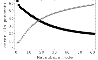
Figure 4: Numerical simulation of the errors (in percent) in the estimate of $\epsilon({\rm i}\xi_{n})-1$ for gold, resulting from using the quantities $I_{\rm exp}(\xi_{n})$ (black squares) and $K_{\rm exp}(\xi_{n})$ (grey triangles) as estimators, in the hypothesis that data are available from $\omega_{\rm min}=0.038$ eV$/\hbar$ to $\omega_{\rm max}=30$ eV$/\hbar$. The integer on the abscissa labels the Matsubara mode $\xi_{n}=2\pi nk_{B}T/\hbar$ ($T=300$ K).

In Fig. 4, we report the relative per cent errors $\delta_{I}=100\,[1-I_{\rm exp}(\xi_{n})/(\epsilon({\rm i}\xi_{n})-1)]$ (black squares) and $\delta_{K}=100\,[1-K_{\rm exp}(\xi_{n})/(\epsilon({\rm i}\xi_{n})-1)]$ (grey triangles) which are made if the quantities $I_{\rm exp}(\xi_{n})$ or $K_{\rm exp}(\xi_{n})$ are used, respectively, as estimators of $\epsilon({\rm i}\xi_{n})-1$. The integer number on the abscissa labels the Matsubara mode $\xi_{n}=2\pi nk_{B}T/\hbar$ ($T=300$ K). Only the first sixty modes are displayed, which are sufficient to estimate the Casimir force at room temperature, for separations larger than 100 nm, with a precision better than one part in ten thousand. As we see, both $I_{\rm exp}(\xi_{n})$ and $K_{\rm exp}(\xi_{n})$ provide a poor approximation to $\epsilon({\rm i}\xi_{n})-1$, with $I_{\rm exp}(\xi_{n})$ performing somehow better at higher imaginary frequencies, and $K_{\rm exp}(\xi_{n})$ doing better at lower imaginary frequencies. Indeed, $I_{\rm exp}(\xi_{n})$ and $K_{\rm exp}(\xi_{n})$ suffer from opposite problems. On one hand the large error affecting $I_{\rm exp}(\xi_{n})$ arises mostly from neglect of the large low-frequency contribution $I_{\rm low}(\xi_{n})$, and to a much less extent from neglect of the high frequency contribution $I_{\rm high}(\xi_{n})$ (The magnitude of the high frequency contribution $I_{\rm high}(\xi_{n})$ is less than two percent of $\epsilon({\rm i}\xi_{n})-1$ for all $n\leq 60$). The situation is quite the opposite in the case of $K_{\rm exp}(\xi_{n})$. This difference is of course due to the opposite limiting behaviors of the imaginary parts of the permittivity $\epsilon^{\prime\prime}(\omega)$ in the limits $\omega\rightarrow 0$, and $\omega\rightarrow\infty$, as compared to those of the imaginary part of the conductivity $\sigma^{\prime\prime}(\omega)$. Indeed, for $\omega\rightarrow 0$, $\epsilon^{\prime\prime}(\omega)$ diverges like $\omega^{-1}$, while $\sigma^{\prime\prime}(\omega)$ approaches zero like $\omega$. This explains while the low frequency contribution $I_{\rm low}(\xi_{n})$ is much larger than $K_{\rm low}(\xi_{n})$. On the other hand, in the limit $\omega\rightarrow\infty$, $\epsilon^{\prime\prime}(\omega)$ vanishes like $\omega^{-3}$, while $\sigma^{\prime\prime}(\omega)$ vanishes only like $\omega^{-1}$. This implies that large frequencies are much less of a problem for $I_{\rm exp}(\xi_{n})$ than for $K_{\rm exp}(\xi_{n})$. The conclusion to be drawn from these considerations is that, if either of the two standard forms Eq. (2) or Eq. (9) of dispersion relations are used, in order to obtain a good estimate of $\epsilon({\rm i}\xi_{n})-1$, one is forced to extrapolate somehow the experimental data both to frequencies less than $\omega_{\rm min}$, and larger than $\omega_{\rm max}$.

We can now consider our windowed dispersion relation, Eq. (7), with our choice of the window functions $f(z)$ in Eq. (10). In Fig. 5, we display the relative per cent error $\delta^{(p,q)}=100\,[1-J_{\rm exp}^{(p,q)}(\xi_{n})/(\epsilon({\rm i}\xi_{n})-1)]$ which is made if the quantity $J_{\rm exp}^{(p,q)}(\xi_{n})$ is used as an estimator of $\epsilon({\rm i}\xi_{n})-1$. We considered two choices of parameters for our window functions in Eq. (10), i.e. $p=1,\,q=2$ (grey triangles) and $p=1,\,q=3$ (black squares). In both cases, we took for the parameter $w$ the constant value $w=(1-2\,{\rm i})\,{\rm eV}/\hbar$ (See Figs. 1, 2 and 3).

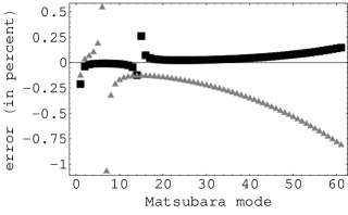
Figure 5: Numerical simulation of the error (in percent) in the estimate of $\epsilon({\rm i}\xi_{n})-1$ for gold, resulting from using the quantity $J_{\rm exp}^{(p,q)}(\xi_{n})$ as a estimator, in the hypothesis that data are available from $\omega_{\rm min}=0.038$ eV$/\hbar$ to $\omega_{\rm max}=30$ eV$/\hbar$. The integer on the abscissa labels the Matsubara mode $\xi_{n}=2\pi nk_{B}T/\hbar$ ($T=300$ K). Grey triangles are for the window function having $p=1,\,q=2$, black squares for $p=1,\,q=3$. In both cases $w=(1-2\,{\rm i})\,{\rm eV}/\hbar$.

It is apparent from Fig. 5 that both window functions perform very well, for all considered Matsubara modes. The error made by using $J_{\rm exp}^{(1,2)}(\xi_{n})$ is less than one percent, in absolute value, while the error made by using $J_{\rm exp}^{(1,3)}(\xi_{n})$ is less than 0.25 percent. The jumps displayed by the relative errors in Fig. 5 (around $n=6$ for the grey dots, and $n=14$ for the black ones) correspond to the approximate positions of the zeroes of the respective window functions $f({\rm i}\xi)$ (see Fig. 3). Such jumps can be easily avoided, further reducing at the same time the error, by making a different choice of the free parameter $w$ for each value of $n$. We did not do this here for the sake of simplicity. It is clear that in concrete cases one is free to choose for each value of $n$, different values of all the parameters $p,q$ and $w$, in such a way that the error is as small as possible.

IV Simulation of the Casimir force

In this Section, we investigate the performance of our window functions with respect to the determination of the Casimir force. We consider for simplicity the prototypical case of two identical plane-parallel homogeneous and isotropic gold plates, placed in vacuum at a distance $a$. As it is well known, the Casimir force per unit area is given by the following Lifshitz formula:

$$P(a,T)=\frac{k_{B}T}{\pi}\sum_{n\geq 0}{\,{}^{\prime}}\int\!\!d{k_{\perp}}{k_{\perp}}q_{n}\!\!\!\!\sum_{\alpha={\rm TE,TM}}\left(\frac{e^{2aq_{n}}}{r_{\alpha}^{2}({\rm i}\xi_{n},{k_{\perp}})}-1\right)^{-1},$$ (27)

where the plus sign corresponds to an attraction between the plates. In this Equation, the prime over the $n$-sum means that the $n=0$ term has to taken with a weight one half, $T$ is the temperature, ${k_{\perp}}$ denotes the magnitude of the projection of the wave-vector onto the plane of the plates and $q_{n}=\sqrt{k_{\perp}^{2}+\xi_{n}^{2}/c^{2}}$, where $\xi_{n}=2\pi n\,k_{B}T/\hbar$ are the Matsubara frequencies. The quantities $r_{\alpha}({\rm i}\xi_{n},{k_{\perp}})$ denote the familiar Fresnel reflection coefficients of the slabs for $\alpha$-polarization, evaluated at imaginary frequencies $i\xi_{n}$. They have the following expressions:

$$r_{\rm TE}({\rm i}\xi_{n},{k_{\perp}})=\frac{q_{n}-k_{n}}{q_{n}+k_{n}}\;,$$ (28)

$$r_{\rm TM}({\rm i}\xi_{n},{\bf k_{\perp}})=\frac{\epsilon({\rm i}\xi_{n})\,q_{n}-k_{n}}{\epsilon({\rm i}\xi_{n})\,q_{n}+k_{n}}\;,$$ (29)

where $k_{n}=\sqrt{k_{\perp}^{2}+\epsilon({\rm i}\xi_{n})\xi_{n}^{2}/c^{2}}$.

We have simulated the error made in the estimate of $P(a,T)$ if the estimate of $\epsilon({\rm i}\xi_{n})$ provided by the window-approximations $J_{\rm exp}^{(p,q)}(\xi_{n})$ is used:

$$\epsilon({\rm i}\xi_{n})\simeq 1+J_{\rm exp}^{(p,q)}(\xi_{n})\;,$$ (30)

again assuming the simple six-oscillator model of Eq. (25) for $\epsilon(\omega)$. The results are summarized in Fig 6, where we plot the relative error $\delta_{P}^{(p,q)}$ in percent, as a function of the separation $a$ (in microns). The window functions that have been used are the same as in Fig. 5.

Figure 6: Simulation of the error (in percent), versus plate separation (in $\mu$m) in the estimate of the Casimir force per unit area, between two plane-parallel gold plates in vacuum at a temperature $T=300K$, resulting from using $J_{\rm exp}^{(p,q)}(\xi_{n})$ as an estimator of $\epsilon({\rm i}\xi_{n})-1$. The window functions are the same as in Fig. 5: the dashed line is for $p=1,q=2$ and the solid line for $p=1,q=3$. All values of the other parameters are same as in Fig. 5.

We see from the figure that already with this simple and not-optimized choice of window functions, the error is much less than one part in a thousand in the entire range of separations considered, from 100 nm to one micron.

V Conclusions and discussion

In recent years, a lot of efforts have been made to measure accurately the Casimir force. At the moment of this writing, the most precise experiments using gold-coated micromechanical oscillators claim a precision better than one percent decca . It is therefore important to see if an analogous level of precision in the prediction of the Casimir force can be obtained at the theoretical level. A precise determination of the theoretical error is indeed as important as reducing the experimental error, in order to address controversial questions that have emerged in the recent literature on dispersion forces, regarding the influence of free charges on the thermal correction to the Casimir force Mohid .

Addressing the theoretical error in the magnitude of the Casimir force is indeed difficult, because many physical effect must be accounted for. However, it has recently been pointed out sveto that perhaps the largest theoretical uncertainty results from incomplete knowledge of the optical data for the surfaces involved in the experiments. On one hand, the large variability depending on the preparation procedure, of the optical properties of gold coatings, routinely used in Casimir experiments, makes it necessary to accurately characterize the coatings actually used in any experiment. On the other hand, even when this characterization is done, another problem arises, because for evaluating the Casimir force one needs to determine the electric permittivity $\epsilon({\rm i}\xi)$ of the coatings for certain imaginary frequencies ${\rm i}\xi$. This quantity is not directly accessible to any optical measurement, and the only way to determine it is via exploiting dispersion relations, that permit to express $\epsilon({\rm i}\xi)$ in terms of the measurable values of the permittivity $\epsilon(\omega)$ for real frequencies $\omega$. When doing this, one is faced with the difficulty that optical data are necessarily known only in a finite interval of frequencies $\omega_{\rm min}<\omega<\omega_{\rm max}$. This practical limitation constitutes a severe problem in the experimentally relevant case of good conductors, because of their large conductivity at low frequencies. With the standard forms of dispersion relations Eq. (2) and Eq. (9), one finds that for practical values of $\omega_{\rm min}$ and $\omega_{\rm max}$, low frequencies less than $\omega_{\rm min}$ and/or large frequencies larger than $\omega_{\rm max}$ give a very large contribution to $\epsilon({\rm i}\xi)$. In order to estimate $\epsilon({\rm i}\xi)$ accurately, one is then forced to extrapolate available optical data outside the experimental region, on the basis of some theoretical model for $\epsilon(\omega)$. Of course, this introduces a further element of uncertainty in the obtained values of $\epsilon({\rm i}\xi)$, and the resulting theoretical error is difficult to estimate quantitatively.

In this paper we have shown that this problem can be resolved by suitably modifying the standard dispersion relation used to compute $\epsilon({\rm i}\xi)$, in terms of appropriate analytic window functions $f(z)$ that suppress the contributions both of low and large frequencies. In this way, it becomes possible to accurately estimate $\epsilon({\rm i}\xi)$ solely on the basis of the available optical data, rendering unnecessary any uncontrollable extrapolation of data. We have checked numerically the performance of simple choices of window functions, by making a numerical simulation based on an analytic fit of the optical properties of gold, that has been used in recent experiments on the Casimir effect Mohid . We found that already very simple forms of the window functions permit to estimate the Casimir pressure with an accuracy better than one part in a thousand, on the basis of reasonable intervals of frequencies for the optical data. It would be interesting to apply these methods to the accurate optical data for thin gold films quoted in Ref. sveto .

Before closing the paper, we should note that the relevance of the sample-to-sample dependence of the optical data observed in sveto for the theory of the Casimir effect has been questioned by the authors of Ref. Mohid , who observed that this dependence mostly originates from relaxation processes of free conduction electrons at infrared and optical frequencies, due for example to different grain sizes in thin films. The main consequence of these sample-dependent features is the large variability of the Drude parameters, extracted from fits of the low-frequency optical data of the films, which constitutes the basic source of variation of the computed Casimir force reported in Ref. sveto . According to the authors of Ref. Mohid , relaxation properties of conduction electrons in thin films, described by the fitted values of the Drude parameters, are not relevant for the Casimir effect. Indeed, according to these authors the quantity $\epsilon(\omega)$ to be used in Lifshitz formula should not be understood as the actual electric permittivity of the plate, as derived from optical measurements on the sample, but it should be rather regarded as a phenomenological quantity connected to but not identical to the optical electric permittivity of the film. The ansatz offered by them for $\epsilon(\omega)$ is dubbed as generalized plasma model, and following Ref. Mohid we denote it as $\epsilon_{\rm gp}(\omega)$. This quantity is a semianalytical mathematical construct, defined by the formula:

$$\epsilon_{\rm gp}(\omega)=\epsilon_{c}(\omega)-\omega_{p}^{2}/\omega^{2}\;,$$ (31)

where $\epsilon_{c}(\omega)$ represents the contribution of core electrons, while the term proportional to the square of the plasma frequency $\omega_{p}$ describes conduction electrons. The most striking qualitative feature of this expression is the neglect of ohmic dissipation in the contribution from conduction electrons, but this is not all. Indeed, the ansatz prescribes that only the core-electron contribution $\epsilon_{c}(\omega)$ should be extracted from optical data of the film. On the contrary, and more importantly, according to Ref. Mohid the value of the plasma frequency $\omega_{p}$ to be used in Eq. (31) should be the one pertaining to a perfect crystal of the ${\it bulk}$ material, and not the one obtained by a Drude-model fit of the low-frequency optical data of the film actually used in the experiment. The justification provided for this choice of the plasma frequency by the authors of Ref. Mohid is that the contribution of conduction electrons to the Casimir force should depend only on properties determined by the structure of the crystal cell, which are independent of the sample-to-sample variability determined by the peculiar grain structure of the film, reported in Ref. sveto . It should be noted that for gold, the value of the plasma frequency advocated in Mohid , $\omega_{p}=9$ eV/$\hbar$, is much higher than the fit values quoted in Ref. sveto , which range from 6.8 to 8.4 eV/$\hbar$. As a result, the approach advocated in Ref. Mohid leads to larger magnitudes of the Casimir force, as compared to the values derived in Ref. sveto , with differences ranging, depending on the sample, from 5 $\%$ to 14 $\%$ at 100 nm. There is no room here to further discuss the merits and faults of these approaches, and we refer the reader to Mohid for a thorough analysis. It is fair to note though that a series of recent experiments by one experimental group decca appears to favor the generalized plasma approach, and to rule out the more conventional approach based on actual optical data followed in Refs. lamor2 ; sveto .

The future will tell what is the correct description. In the meanwhile, we remark that whatever approach is followed, the methods proposed in this paper may prove useful to obtain more reliable estimates of the Casimir force for future experiments.

Acknowledgements The author thanks the ESF Research Network CASIMIR for financial support.

References

- (1) H. B. G. Casimir, Proc. K. Ned. Akad. Wet. Rev. 51, 793 (1948).
- (2) E. M. Lifshitz, Sov. Phys. JETP 2, 73 (1956); E. M. Lifshitz and L. P. Pitaevskii, Landau and Lifshitz Course of Theoretical Physics: Statistical Physics Part II (Butterworth-Heinemann, 1980).
- (3) S. K. Lamoreaux, Phys. Rev. Lett. 78, 5 (1997); 81, 5475 (1998).
- (4) U. Mohideen and A. Roy, Phys. Rev. Lett. 81, 4549 (1998); A. Roy, C.-Y. Lin, and U. Mohideen, Phys. Rev D 60, 111101(R) (1999).
- (5) G. Bressi, G. Carugno, R. Onofrio, and G. Ruoso, Phys. Rev. Lett. 88, 041804 (2002).
- (6) T. Ederth, Phys. Rev. A 62, 062104 (2000).
- (7) H. B. Chan, Y. Bao, J. Zou, R. A. Cirelli, F. Klemens, W. M. Mansfield, and C. S. Pai, Phys. Rev. Lett. 101, 030401 (2008).
- (8) H. B. Chan, V.A. Aksyuk, R.N. Kleiman, D.J. Bishop, and F. Capasso, Science 291, 1941 (2001).
- (9) F. Chen, G. L. Klimchitskaya, V. M. Mostepanenko, and U. Mohideen, Opt. Expr. 15, 4823 (2007); Phys. Rev. B 76, 035338 (2007).
- (10) S. de Man, K. Heeck, R. J. Wijngaarden, and D. Iannuzzi, Phys. Rev. Lett. 103, 040402 (2009).
- (11) G. Bimonte, E. Calloni, G. Esposito, L. Milano, and L. Rosa, Phys. Rev. Lett. 94, 180402 (2005); G. Bimonte, E. Calloni, G. Esposito, and L. Rosa, Nucl. Phys. B 726, 441 (2005); G. Bimonte et al., J. Phys. A 41, 164023 (2008); G. Bimonte, Phys. Rev. A 78, 062101 (2008).
- (12) G. L. Klimchitskaya, U. Mohideen, and V. M. Mostepanenko, Rev. Mod. Phys. 81, 1827 (2009).
- (13) R.S. Decca, D. Lopez, E. Fischbach, G.L. Klimchitskaya, D.E. Krause, and V.M. Mostepanenko, Ann. Phys. 318, 37 (2005); Eur. Phys. J. C 51, 963 (2007), Phys. Rev. D 75, 077101 (2007).
- (14) A. Lambrecht and S. Reynaud, Eur. Phys. J. D 8, 309 (2000).
- (15) A. Naji, D. S. Dean, J. Sarabadani, R. R. Horgan, and R. Podgornik, Phys. Rev. Lett. 104, 060601 (2010).
- (16) Handbook of Optical Constants of Solids, edited by E. D. Palik (Academic, New York, 1995).
- (17) S. K. Lamoreaux, Phys. Rev. A 59, R3149 (1999).
- (18) I. Pirozhenko, A. Lambrecht, and V. B. Svetovoy, New. J. Phys. 8, 238 (2006).
- (19) V. B. Svetovoy, P. J. van Zwol, G. Palasantzas, and J. Th. M. De Hosson, Plys. Rev. B 77, 035439 (2008).
- (20) T. Emig, N. Graham, R. L. Jaffe, and M. Kardar, Phys. Rev. Lett. 99, 170403 (2007); Phys. Rev. D 77, 025005 (2008).
- (21) O. Kenneth and I. Klich, Phys. Rev. B 78, 014103 (2008).
- (22) A. Lambrecht, P. A. Maia Neto, and S. Reynaud, New. J. Phys. 8, 243 (2006).
- (23) L. D. Landau, and E. M. Lifshitz, Landau and Lifshitz Course of Theoretical Physics: Electrodynamics of Continuous Media (Pergamon Press, New York, 1960).
- (24) G. Bimonte, H. Haakh, C. Henkel, and F. Intravaia, arXiv:0907.3775v2 (in press on J. Phys. A)