Fast algorithms for computing isogenies between ordinary elliptic curves in small characteristic

Abstract

The problem of computing an explicit isogeny between two given elliptic curves over $\mathbb{F}_{q}$, originally motivated by point counting, has recently awaken new interest in the cryptology community thanks to the works of Teske and Rostovstev & Stolbunov.

While the large characteristic case is well understood, only suboptimal algorithms are known in small characteristic; they are due to Couveignes, Lercier, Lercier & Joux and Lercier & Sirvent. In this paper we discuss the differences between them and run some comparative experiments. We also present the first complete implementation of Couveignes’ second algorithm and present improvements that make it the algorithm having the best asymptotic complexity in the degree of the isogeny.

1 Introduction

The problem of computing an explicit degree $\ell$ isogeny between two given elliptic curves over $\mathbb{F}_{q}$ was originally motivated by point counting methods based on Schoof’s algorithm [1], [11], [26]. A review of the most efficient algorithms to solve this problem is given in [4] together with a new quasi-optimal algorithm; however, all the algorithms presented in [4] are limited to the case $\ell\ll p$ where $p$ is the characteristic of $\mathbb{F}_{q}$. This is satisfactory for cryptographic applications where one takes $p=q$ or $p=2$; indeed in the former case Schoof’s algorithm needs $\ell\in O(\log p)$, while in the latter case there’s no need to compute explicit isogenies since $p$-adic methods based on [25] are preferred to Schoof’s algorithm.

Nevertheless, the problem of computing explicit isogenies in the case where $p$ is small compared to $\ell$ remains of theoretical interest and can find practical applications in newer cryptosystems such as [28], [24]. The first algorithm to solve this problem was given by Couveignes and made use of formal groups [7]; it takes $\tilde{O}(\ell^{3}\log q)$ operations in $\mathbb{F}_{p}$ assuming $p$ is constant, however it has an exponential complexity in $\log p$. Another algorithm by Lercier specific to $p=2$ uses some linear properties of the problem to build a linear system from whose solution the isogeny can be deduced [20]; its complexity is conjectured to be $\tilde{O}(\ell^{3}\log q)$ operations in $\mathbb{F}_{p}$, but it has a much better constant factor than [7]. At the moment we write, the latter algorithm is by many orders of magnitude the fastest algorithm to solve practical instances of the problem when $p=2$, thus being the de facto standard for cryptographic use.

$p$-adic methods were used by Joux and Lercier [13] and Lercier and Sirvent [22] to solve the isogeny problem. The former method has complexity $\tilde{O}(\ell^{2}(1+\ell/p)\log q)$ operations in $\mathbb{F}_{p}$, which makes it well adapted to the case where $p\sim\log q$. The latter has complexity $\tilde{O}(\ell^{3}+\ell\log q^{2})$ operations in $\mathbb{F}_{p}$, making it the best algorithm to our knowledge for the case where $p$ is not constant.

The algorithm C2 and its variants

Finally, the algorithm having the best asymptotic complexity in $\ell$ was proposed again by Couveignes in [8]; we will refer to this original version as “C2”. Its complexity –supposing $p$ is fixed– was estimated in [8] as being $\tilde{O}(\ell^{2}\log q)$ operations in $\mathbb{F}_{p}$, but with a precomputation step requiring $\tilde{O}(\ell^{3}\log q)$ operations and large memory requirements. However, some more work is needed to effectively reach these bounds, while a straightforward implementation of C2 has an overall asymptotic complexity of $\tilde{O}(\ell^{3}\log q)$ operations, as we will argue in Section 3.

Subsequent work by Couveignes [9], and more recently [10], use Artin-Schreier theory to avoid the precomputation step of C2 and drop the memory requirements to $\tilde{O}(\ell\log q+\log^{2}q)$ elements of $\mathbb{F}_{p}$. However, this is still not enough to reduce the overall complexity of the algorithm, as we will argue in Section 4. We refer to this variant as “C2-AS”.

In the present paper we give a complete review of Couveignes’ algorithm, we present new variants that reach the foreseen quadratic bound in $\ell^{2}$ and prove an accurate complexity estimate which doesn’t suppose $p$ to be fixed. We also run experiments to compare the performances of C2 with other algorithms.

Notation and plan

In the rest of the paper $p$ is a prime, $d$ a positive integer, $q=p^{d}$ and $\mathbb{F}_{q}$ is the field with $q$ elements. For an elliptic curve $E$ and a field $\mathbb{K}$ embedded in an algebraic closure $\bar{\mathbb{K}}$, we note by $E(\mathbb{K})$ the set of $\mathbb{K}$-rational points and by $E[m]$ the $m$-torsion subgroup of $E(\bar{\mathbb{K}})$. The group law on the elliptic curve is noted additively, its zero is the point at infinity, noted $\mathcal{O}$. For an affine point $P$ we note by $x(P)$ its abscissa and by $y(P)$ its ordinate. We will restrict ourselves to the case of ordinary elliptic curves, thus $E[p^{k}]\cong\mathbb{Z}/p^{k}\mathbb{Z}$.

Unless otherwise stated, all time complexities will be measured in number of operations in $\mathbb{F}_{p}$ and all space complexities in number of elements of $\mathbb{F}_{p}$; we do not assume $p$ to be constant. We use the $O$, $\Theta$ and $\Omega$ notations to state respectively upper bounds, tight bounds and lower bounds for asymptotic complexities. We also use the notation $\tilde{O}_{x}$ that forgets polylogarithmic factors in the variable $x$, thus $O(xy\log x\log y)\subset\tilde{O}_{x}(xy\log y)\subset\tilde{O}_{x,y}(xy)$. We simply note $\tilde{O}$ when the variables are clear from the context.

We let $2<\omega\leqslant 3$ be the exponent of linear algebra, that is an integer such that $n\times n$ matrices can be multiplied in $n^{\omega}$ operations. We let $\mathrm{\sf M}:\mathbb{N}\rightarrow\mathbb{N}$ be a multiplication function, such that polynomials of degree at most $n$ with coefficients in $\mathbb{F}_{p}$ can be multiplied in $\mathrm{\sf M}(n)$ operations, under the conditions of [14, Ch. 8.3]. Typical orders of magnitude are $O(n^{\log_{2}3})$ for Karatsuba multiplication or $O(n\log n\log\log n)$ for FFT multiplication. Similarly, we let $\mathrm{\sf C}:\mathbb{N}\rightarrow\mathbb{N}$ be the complexity of modular composition, that is a function such that $\mathrm{\sf C}(n)$ is the number of field operations needed to compute $f\circ g\bmod h$ for $f,g,h\in\mathbb{K}[X]$ of degree at most $n$ with coefficients in an arbitrary field $\mathbb{K}$. The best known algorithm is [2], this implies $\mathrm{\sf C}(n)\in O\left(n^{\frac{\omega+1}{2}}\right)$. Note that in a boolean RAM model, the algorithm of [19] takes quasi-linear time.

Organisation of the paper

In Section 2 we give preliminaries on elliptic curves and isogenies. In Sections 3 through 6 we develop the algorithm C2 and we incrementally improve it by giving a new faster variant in each Section. Section 7 gives technical details on our implementations of the algorithms of this paper and of [22]. Finally in Section 8 we comment the results of the experiments we ran on our implementations.

2 Preliminaries on Isogenies

Let $E$ be an ordinary elliptic curve over the field $\mathbb{F}_{q}$. We suppose it is given to us as the locus of zeroes of an affine Weierstrass equation

$$y^{2}+a_{1}xy+a_{3}y=x^{3}+a_{2}x^{2}+a_{4}x+a_{6}\qquad a_{1},\ldots,a_{6}\in\mathbb{F}_{q}\text{.}$$

Simplified forms

If $p>3$ it is well known that the curve $E$ is isomorphic to a curve in the form

$$y^{2}=x^{3}+ax+b$$ (1)

and its $j$-invariant is $j(E)=\frac{1728(4a)^{3}}{16(4a^{3}+27b^{2})}$.

When $p=3$, since $E$ is ordinary, it is isomorphic to a curve

$$y^{2}=x^{3}+ax^{2}+b$$ (2)

and its $j$-invariant is $j(E)=-\frac{a^{3}}{b}$.

Finally, when $p=2$, since $E$ is ordinary, it is isomorphic to a curve

$$y^{2}+xy=x^{3}+ax^{2}+b$$ (3)

and its $j$-invariant is $j(E)=\frac{1}{b}$.

These isomorphism are easy to compute and we will always assume that the elliptic curves given to our algorithms are in such simplified forms.

Isogenies

Elliptic curves are endowed with the classic group structure through the chord-tangent law. A group morphism having finite kernel is called an isogeny. Isogenies are regular maps, as such they can be represented by rational functions. An isogeny is said to be $\mathbb{K}$-rational if it is $\mathbb{K}$-rational as regular map; its degree is the degree of the regular map.

One important property about isogenies is that they factor the multiplication-by-$m$ map.

Definition 1 (Dual isogeny).

Let $\mathcal{I}:E\rightarrow E^{\prime}$ be a degree $m$ isogeny. There exists an unique isogeny $\hat{\mathcal{I}}:E^{\prime}\rightarrow E$, called the dual isogeny such that

$$\mathcal{I}\circ\hat{\mathcal{I}}=[m]_{E}\qquad\text{and}\qquad\hat{\mathcal{I}}\circ\mathcal{I}=[m]_{E^{\prime}}$$

As regular maps, isogenies can be separable, inseparable or purely inseparable. In the case of finite fields, purely inseparable isogenies are easily understood as powers of the frobenius map. Let

$$E^{(p)}:y^{2}+a_{1}^{p}xy+a_{3}^{p}y=x^{3}+a_{2}^{p}x^{2}+a_{4}^{p}x+a_{6}^{p}$$

then the map

$$\phi:E \rightarrow E^{(p)}$$

$$(x,y) \mapsto(x^{p},y^{p})$$

is a degree $p$ purely inseparable isogeny. Any purely inseparable isogeny is a composition of such frobenius isogenies.

Let $E$ and $E^{\prime}$ be two elliptic curves defined over $\mathbb{F}_{q}$, by finding an explicit isogeny we mean to find an ($\mathbb{F}_{q}$-rational) rational function from $E(\bar{\mathbb{F}}_{q})$ to $E^{\prime}(\bar{\mathbb{F}}_{q})$ such that the map it defines is an isogeny.

Figure 1: Factorization of an isogeny. $\mathcal{I}^{\prime}$ has kernel $E[m]\oplus\ker\mathcal{I}$.

Since an isogeny can be uniquely factored in the product of a separable and a purely inseparable isogeny, we focus ourselves on the problem of computing explicit separable isogenies. Furthermore one can factor out multiplication-by-$m$ maps, thus reducing the problem to compute explicit separable isogenies with cyclic kernel (see figure 1).

In the rest of this paper, unless otherwise stated, by $\ell$-isogeny we mean a separable isogeny with kernel isomorphic to $\mathbb{Z}/\ell\mathbb{Z}$.

Vélu formulae

For any finite subgroup $G\subset E(\bar{\mathbb{K}})$, Vélu formulae [29] give in a canonical way an elliptic curve $\bar{E}$ and an explicit isogeny $\mathcal{I}:E\rightarrow\bar{E}$ such that $\ker\mathcal{I}=G$. The isogeny is $\mathbb{K}$-rational if and only if the polynomial vanishing on the abscissae of $G$ belongs to $\mathbb{K}[X]$.

In practice, if $E$ is defined over $\mathbb{F}_{q}$ and if

$$h(X)=\prod_{\begin{subarray}{c}P\in G\\ P\neq\mathcal{O}\end{subarray}}(X-x(P))\in\mathbb{F}_{q}[X]$$

is known, Vélu formulae compute a rational function

$$\bar{\mathcal{I}}(x,y)=\left(\frac{g(x)}{h(x)},\frac{k(x,y)}{l(x)}\right)$$ (4)

and a curve $\bar{E}$ such that $\bar{\mathcal{I}}:E\rightarrow\bar{E}$ is an $\mathbb{F}_{q}$-rational isogeny of kernel $G$. A consequence of Vélu formulae is

$$\deg g=\deg h+1=\#G\text{.}$$ (5)

Given two curves $E$ and $E^{\prime}$, Vélu formulae reduce the problem of finding an explicit isogeny between $E$ and $E^{\prime}$ to that of finding the kernel of an isogeny between them. Once the polynomial $h(X)$ vanishing on $\ker\mathcal{I}$ is found, the explicit isogeny is computed composing Vélu formulae with the isomorphism between $\bar{E}$ and $E^{\prime}$ as in figure 2.

Figure 2: Using Vélu formulae to compute an explicit isogeny.

3 The algorithm C2

The algorithm we refer to as C2 was originally proposed in [8]. It takes as input two elliptic curves $E,E^{\prime}$ and an integer $\ell$ prime to $p$ and it returns, if it exists, an $\mathbb{F}_{q}$-rational isogeny of degree $\ell$ between $E$ and $E^{\prime}$. It only works in odd characteristic.

3.1 The original algorithm

Suppose there exists an $\mathbb{F}_{q}$-rational isogeny $\mathcal{I}:E\rightarrow E^{\prime}$ of degree $\ell$. Since $\ell$ is prime to $p$ one has $\mathcal{I}(E[p^{k}])=E^{\prime}[p^{k}]$ for any $k$.

Recall that $E[p^{k}]$ and $E^{\prime}[p^{k}]$ are cyclic groups. C2 iteratively computes generators $P_{k},P_{k}^{\prime}$ of $E[p^{k}]$ and $E^{\prime}[p^{k}]$ respectively. Now C2 makes the guess $\mathcal{I}(P_{k})=P_{k}^{\prime}$; then, if $\mathcal{I}$ is given by rational fractions as in (4),

$$\frac{g\bigl{(}x([i]P_{k})\bigr{)}}{h\bigl{(}x([i]P_{k})\bigr{)}}=x([i]P_{k}^{\prime})\quad\text{for $i\in\mathbb{Z}/p^{k}\mathbb{Z}$}$$ (6)

and by (5) $\deg g=\deg h+1=\ell$.

Using (6) one can compute the rational fraction $\frac{g(X)}{h(X)}$ through Cauchy interpolation over the points of $E[p^{k}]$ for $k$ large enough. C2 takes $p^{k}>4\ell-2$, interpolates the rational fraction and then checks that it corresponds to the restriction of an isogeny to the $x$-axis. If this is the case, the whole isogeny is computed through Vélu formulae and the algorithm terminates. Otherwise the guess $\mathcal{I}(P_{k})=P_{k}^{\prime}$ was wrong, then C2 computes a new generator for $E^{\prime}[p^{k}]$ and starts over again.

We now go through the details of the algorithm.

The $p$-torsion

The computation of the $p$-torsion points follows from the work of Gunji [16]. Here we suppose $p\neq 2$.

Definition 2.

Let $E$ have equation $y^{2}=f(x)$. The Hasse invariant of $E$, noted $H_{E}$, is the coefficient of $X^{p-1}$ in $f(X)^{\frac{p-1}{2}}$.

Gunji shows the following proposition and gives formulae to compute the $p$-torsion points.

Proposition 3.

Let $c=\sqrt[p-1]{H_{E}}$; then, the $p$-torsion points of $E$ are defined in $\mathbb{F}_{q}[c]$ and their abscissae are defined in $\mathbb{F}_{q}[c^{2}]$.

The $p^{k}$-torsion

$p^{k}$-torsion points are iteratively computed via $p$-descent. The basic idea is to split the multiplication map as $[p]=\phi\circ V$ and invert each of the components. The purely inseparable isogeny $\phi$ is just a frobenius map and the separable isogeny $V$ can be computed by Vélu formulae once the $p$-torsion points are known. Although this is reasonably efficient, pulling $V$ back may involve factoring polynomials of degree $p$ in some extension field.

A finer way to do the $p$-descent, as suggested in the original paper [8], is to use the work of Voloch [30]. Suppose $p\neq 2$, let $E$ and $\widetilde{E}$ have equations respectively

$$y^{2} =f(x)=x^{3}+a_{2}x^{2}+a_{4}x+a_{6}\;\text{,}$$

$$\tilde{y}^{2} =\tilde{f}(\tilde{x})=\tilde{x}^{3}+\sqrt[p]{a_{2}}\tilde{x}^{2}+\sqrt[p]{a_{4}}\tilde{x}+\sqrt[p]{a_{6}}\;\text{,}$$

set

$$\tilde{f}(X)^{\frac{p-1}{2}}=\alpha(X)+H_{\widetilde{E}}X^{p-1}+X^{p}\beta(X)$$ (7)

with $\deg\alpha<p-1$ and $H_{\widetilde{E}}$ the Hasse invariant of $\widetilde{E}$. Voloch shows the following proposition.

Proposition 4.

Let $\tilde{c}=\sqrt[p-1]{H_{\widetilde{E}}}$, the cover of $\widetilde{E}$ defined by

$$C:\;\tilde{z}^{p}-\tilde{z}=\frac{\tilde{y}\beta(\tilde{x})}{\tilde{c}^{p}}$$ (8)

is an étale cover of degree $p$ and is isomorphic to $E$ over $\mathbb{F}_{q}[\tilde{c}]$; the isomorphism is given by

$$\left\{\begin{aligned} (\tilde{x},\tilde{y})&=V(x,y)\\ \tilde{z}&=-\frac{y}{\tilde{c}^{p}}\sum_{i=1}^{p-1}\frac{1}{x-x([i]P_{1})}\end{aligned}\right.$$ (9)

where $P_{1}$ is a primitive $p$-torsion point of $E$.

The descent is then performed as follows: starting from a point $P$ on $E$, first pull it back along $\phi$, then take one of its pre-images in $C$ by solving equation (8), finally use equation (9) to land on a point $P^{\prime}$ in $E$. The proposition guarantees that $[p]P^{\prime}=P$. The descent is pictured in figure 3.

      

Figure 3: Two ways of doing the $p$-descent: standard on the left and via a degree $p$ cover on the right

The reason why this is more efficient than a standard descent is the shape of equation (8): it is an Artin-Schreier equation and it can be solved by many techniques, the simplest being linear algebra (as was suggested in [8]). Once a solution $\tilde{z}$ to (8) is known, solving in $x$ and $y$ the bivariate polynomial system (9) takes just a GCD computation (explicit formulae were given by Lercier in [21, $\S$6.2], we give some slightly improved ones in Section 7). Compare this with a generic factoring algorithm needed by standard descent.

Solving Artin-Schreier equations is the most delicate task of the descent and we will further discuss it.

Cauchy interpolation

Interpolation reconstructs a polynomial from the values it takes on some points; Cauchy interpolation reconstructs a rational fraction. The Cauchy interpolation algorithm is divided in two phases: first find the polynomial $P$ interpolating the evaluation points, then use rational fraction reconstruction to find a rational fraction congruent to $P$ modulo the polynomial vanishing on the points. The first phase is carried out through any classical interpolation algorithm, while the second is similar to an XGCD computation. See [14, $\S$5.8] for details.

Cauchy interpolation needs $n+2$ points to reconstruct a degree $(k,n-k)$ rational fraction. This, together with (5), justifies the choice of $k$ such that $p^{k}>4\ell-2$. Some of our variants of C2 will interpolate only on the primitive $p^{k}$-torsion points, thus requiring the slightly larger bound $\phi(p^{k})\geqslant 4\ell-2$. This is not very important to our asymptotical analysis since in both cases $p^{k}\in O(\ell)$.

Recognising the isogeny

Once the rational fraction $\frac{g(X)}{h(X)}$ has been computed, one has to verify that it is indeed an isogeny. The first test is to check that the degrees of $g$ and $h$ match equation (5), if they don’t, the equation can be discarded right away and the algorithm can go on with the next trial. Next, one can check that $h$ is indeed the square of a polynomial (or, if $\ell$ is even, the product of one factor of the $2$-division polynomial and a square polynomial). This two tests are usually enough to detect an isogeny, but, should they lie, one can still check that the resulting rational function is indeed a group morphism by trying some random points on $E$.

3.2 The case $p=2$

The algorithm as we have presented it only works when $p\neq 2$, it is however an easy matter to generalise it. The only phase that doesn’t work is the computation of the $p^{k}$-torsion points. For curves in the form (3) the only $2$-torsion point is $(0,\sqrt{b})$.

Voloch formulae are hard to adapt, nevertheless a $2$-descent on the Kummer surface of $E$ can easily be performed since the doubling formula reads

$$x([2]P)=\frac{b}{x(P)^{2}}+x(P)^{2}=\phi\left(\frac{\sqrt{b}+x(P)^{2}}{x(P)}\right)=\phi\circ V\;\text{.}$$ (10)

Given point $x_{P}$ on $K_{E}$, a pull-back along $\phi$ gives a point $\tilde{x}_{P}$ on $K_{\widetilde{E}}$. Then pulling $V$ back amounts to solve

$$x^{2}+\tilde{x}_{P}x=\sqrt{b}$$ (11)

and this can be turned in an Artin-Schreier equation through the change of variables $x\rightarrow x^{\prime}\tilde{x}_{P}$.

From the descent on the Kummer surfaces one could deduce a full $2$-descent on the curves by solving a quadratic equation at each step in order recover the $y$ coordinate, but this would be too expensive. Fortunately, the $y$ coordinates are not needed by the subsequent steps of the algorithm, thus one may simply ignore them. Observe in fact that even if $K_{E}$ does not have a group law, the restriction of scalar multiplication is well defined and can be computed through Montgomery formulae [23]. This is enough to compute all the abscissae of the points in $E[p^{k}]$ once a generator is known.

3.3 Complexity analysis

Analysing the complexity of C2 is a delicate matter since the algorithm relies on some black-box computer algebra algorithms in order to deal with finite extensions of $\mathbb{F}_{q}$. The choice of the actual algorithms may strongly influence the overall complexity of C2. In this section we will only give some lower bounds on the complexity of C2, since a much more accurate complexity analysis will be carried out in Section 4.

$p$-torsion

Applying Gunji formulae first requires to find $c$ and $c^{\prime}$, $p-1$-th roots of $H_{E}$ and $H_{E^{\prime}}$, and build the field extension $\mathbb{F}_{q}[c]=\mathbb{F}_{q}[c^{\prime}]$. Independently of the actual algorithm used, observe that in the worst case $\mathbb{F}_{q}[c]$ is a degree $p-1$ extension of $\mathbb{F}_{q}$, thus simply representing one of its elements requires $\Theta(pd)$ elements of $\mathbb{F}_{p}$.

Subsequently, the main cost in Gunji’s formulae is the computation of the determinant of a $\frac{p-1}{2}\times\frac{p-1}{2}$ quadri-diagonal matrix (see [16]). This takes $\Theta(p^{2})$ operations in $\mathbb{F}_{q}[c]$ by Gauss elimination, that is no less than $\Omega(p^{3}d)$ operations in $\mathbb{F}_{p}$.

$p^{k}$-torsion

During the $p$-descent, factoring of equations (8) or (11) may introduce some field extensions over $\mathbb{F}_{q}[c]$. Observe that an Artin-Schreier polynomial is either irreducible or totally split, so at each step of the $p$-descent we either stay in the same field or we take a degree $p$ extension. This shows that in the worst case, we have to take an extension of degree $p^{k-1}$ over $F_{q}[c]$. The following proposition, which is a generalisation of [21, Prop. 26], states precisely how likely this case is.

Proposition 5.

Let $E$ be an elliptic curve over $\mathbb{F}_{q}$, we note $\mathbb{U}_{i}$ the smallest field extension of $\mathbb{F}_{q}$ such that $E[p^{i}]\subset E(\mathbb{U}_{i})$. For any $i\geqslant 1$, either $[\mathbb{U}_{i+1}:\mathbb{U}_{i}]=p$ or $\mathbb{U}_{i+1}=\mathbb{U}_{i}=\cdots=\mathbb{U}_{1}$.

Proof.

Observe that the action of the Frobenius $\phi$ on $E[p]$ is just multiplication by the trace $t$, in fact the equation

$$\phi^{2}-[t\bmod p]\circ\phi+[q\bmod p]=0$$

has two solutions, namely $[t\bmod p]$ and $[0\bmod p]$, but the second can be discarded since it would imply that $\phi$ has non-trivial kernel. By lifting this solution, one sees that the action of $\phi$ on the Tate module $\mathcal{T}_{p}(E)$ is equal to multiplication by some $\tau\in\mathbb{Z}_{p}$.

Note $G$ the absolute Galois group of $\mathbb{F}_{q}$, there is a well known action of $G$ on $\mathcal{T}_{p}(E)$. Since $G$ is generated by the Frobenius automorphism of $\mathbb{F}_{q}$, the restriction of this action to $E[p^{k}]$ is equal to the action (via multiplication) of the subgroup of $(\mathbb{Z}/p^{k}\mathbb{Z})^{\ast}$ generated by $\tau_{k}=\tau\bmod p^{k}$. Hence $[\mathbb{U}_{k}:\mathbb{F}_{q}]=\operatorname{ord}(\tau_{k})$.

Then, for any $k>1$, [21, Corollary 4] applied to $\tau_{k+1}=\tau\bmod p^{k+1}$ shows that $\operatorname{ord}(\tau_{k+1})=\operatorname{ord}(\tau_{k})$ implies $\operatorname{ord}(\tau_{k})=\operatorname{ord}(\tau_{k-1})$ and this concludes the proof. ∎

Thus for any elliptic curve there is an $i_{0}$ such that $[\mathbb{U}_{i}:\mathbb{U}_{1}]=p^{i-i_{0}}$ for any $i\geqslant i_{0}$. This shows that the worst and the average case coincide since for any fixed curve $[\mathbb{U}_{k}:\mathbb{U}_{1}]\in\Theta(p^{k})$ asymptotically. In this situation, one needs $\Theta(p^{k}d)$ elements of $\mathbb{F}_{p}$ to store an element of $\mathbb{U}_{k}$.

Now the last iteration of the $p$-descent needs to solve an Artin-Schreier equation in $\mathbb{U}_{k}$. To do this C2 precomputes the matrix of the $\mathbb{F}_{q}$-linear application $(x^{q}-x):\mathbb{U}_{k}\rightarrow\mathbb{U}_{k}$ and its inverse, plus the matrix of the $\mathbb{F}_{p}$-linear application $(x^{p}-x):\mathbb{F}_{q}\rightarrow\mathbb{F}_{q}$ and its inverse. The former is the most expensive one and takes $\Theta(p^{\omega k})$ operations in $\mathbb{F}_{q}$, that is $\Omega(p^{\omega k}d)=\Omega(\ell^{\omega}d)$ operations in $\mathbb{F}_{p}$, plus a storage of $\Theta(\ell^{2}d)$ elements of $\mathbb{F}_{p}$. Observe that this precomputation may be used to compute any other isogeny with domain $E$.

After the precomputation has been done, C2 successively applies the two inverse matrices; details can be found in [8, $\S$2.4]. This costs at least $\Omega(\ell^{2}d)$.

Interpolation

The most expensive part of Cauchy interpolation is the polynomial interpolation phase. In fact, simply representing a polynomial of degree $p^{k}-1$ in $\mathbb{U}_{k}[X]$ takes $\Theta(p^{2k}d)$ elements, thus at least $\Omega(\ell^{2}d)$ operations are needed to interpolate unless special care is taken. This contribution due to arithmetics in $\mathbb{U}_{k}$ had been underestimated in the complexity analysis of [8], which gave an estimate of $\Omega(\ell d\log\ell)$ operations for this phase. We will give more details on interpolation in Section 5.

Recognising the isogeny

The cost of testing for squareness of the denominator and other tests is negligible compared to the rest of the algorithm. Nevertheless it is important to realize that on average half of the $\phi(p^{k})$ mappings from $E[p^{k}]$ to $E^{\prime}[p^{k}]$ must be tried before finding the isogeny, for only one of these mappings corresponds to it. This implies that the Cauchy interpolation step must be repeated an average of $\Theta(p^{k})$ times, thus contributing a $\Omega(\ell^{3}d)$ to the total complexity.

Summing up all the contributions one ends up with the following lower bound

$$\Omega(\ell^{3}d+p^{3}d)$$ (12)

plus a precomputation step whose cost is negligible compared to this one and a space requirement of $\Theta(\ell^{2}d)$ elements. In the next sections we will see how to make all these costs drop.

4 The algorithm C2-AS

One of the most expensive steps of C2 is the resolution of an Artin-Schreier equation in an extension field $\mathbb{U}_{i}$. In [9] Couveignes gives an approach alternative to linear algebra to solve this problem. First it builds the whole tower $(\mathbb{U}_{1}=\mathbb{F}_{q}[c],\ldots,\mathbb{U}_{k})$ of intermediate extensions, then it solves an Artin-Schreier equation in $\mathbb{U}_{i}$ recursively by reducing it to another Artin-Schreier equation in $\mathbb{U}_{i}$. Details are in [9] and [10].

To solve the final Artin-Schreier equation in $\mathbb{U}_{1}=\mathbb{F}_{q}[c]$ one resorts to linear algebra, thus precomputing the inverse matrix of the $\mathbb{F}_{p}$-linear application $(x^{p}-x):\mathbb{U}_{1}\rightarrow\mathbb{U}_{1}$.

4.1 Complexity analysis

How effective this method is depends on the way algebra is performed in the tower $(\mathbb{U}_{1},\ldots,\mathbb{U}_{k})$. The present author and Schost [10] recently presented a new construction based on Artin-Schreier theory that allows to do most arithmetic operations in the tower in quasi-linear time. Assuming this construction is used, we can now give precise bounds for each step of C2-AS.

$p$-torsion

The construction of $\mathbb{F}_{q}[c]$ may be done in many ways. The only requirements of [10] are

1. that its elements have a representation as elements of $F_{p}[X]/Q_{1}(X)$ for some irreducible polynomial $Q_{1}$,

2. that either $(d,p)=1$ or $\deg Q_{1}^{\prime}+2=\deg Q_{1}$.

Selecting a random polynomial $Q_{1}$ and testing for irreducibility is usually enough to meet these conditions. This costs $O\bigl{(}pd\mathrm{\sf M}(pd)\log(pd)\log(p^{2}d)\bigr{)}$ according to [14, Th. 14.42].

Now we need to compute the embedding $\mathbb{F}_{q}\subset\mathbb{F}_{q}[c]$. Supposing $\mathbb{F}_{q}$ is represented as $\mathbb{F}_{p}[X]/Q_{0}(X)$, we factor $Q_{0}$ in $\mathbb{F}_{q}[c]$, which costs $O\bigl{(}pd\mathrm{\sf M}(pd^{2})\log d\log p\bigr{)}$ using [14, Coro. 14.16]. Then the most naive technique to express the embedding is linear algebra. This requires the computation of $pd$ elements of $\mathbb{F}_{q}[c]$ at the expense of $\Theta\bigl{(}pd\mathrm{\sf M}(pd)\bigr{)}$ operations in $\mathbb{F}_{p}$, then the inversion of the matrix holding such elements, at a cost of $\Theta\bigl{(}(pd)^{\omega}\bigr{)}$ operations. This is certainly not optimal, yet this phase will have negligible cost compared to the rest of the algorithm.

Now we can compute $c$ and $c^{\prime}$ by factoring the polynomials $Y^{p-1}-H_{E}$ and $Y^{p-1}-H_{E^{\prime}}$ in $\mathbb{F}_{p}[X]/Q_{1}(X)$. This costs

$$O\bigl{(}(p\mathrm{\sf C}(pd)+\mathrm{\sf C}(p)\mathrm{\sf M}(pd)+\mathrm{\sf M}(p)\mathrm{\sf M}(pd)\log p)(\log^{2}p+\log d)\bigr{)}$$

using [17, Section 3].

Finally, computing the determinants needed by Gunji’s formulae takes $\Theta(p^{2})$ multiplications in $\mathbb{F}_{q}[c]$, that is $\Theta\bigl{(}p^{2}\mathrm{\sf M}(pd)\bigr{)}$.

Letting out logarithmic factors, the overall cost of this phase is

$$\tilde{O}\bigl{(}p^{2}d^{3}+p\mathrm{\sf C}(pd)+\mathrm{\sf C}(p)pd+(pd)^{\omega}\bigr{)}$$ (13)

$p^{k}$-torsion

Application of Voloch formulae requires at each of the levels $\mathbb{U}_{2},\ldots,\mathbb{U}_{k}$

1. to solve equation (8) by factoring an Artin-Schreier polynomial,

2. to solve the system (9).

If we assume the worst case $[\mathbb{U}_{2}:\mathbb{U}_{1}]=p$, according to [10, Th. 13], at each level $i$ the first step costs

$$O\bigl{(}(pd)^{\omega}i+{\sf PT}(i-1)+\mathrm{\sf M}(p^{i+1}d)\log p\bigr{)}$$

$$\begin{aligned} \text{where}&&{\sf PT}(i)&=O\bigl{(}(pi+\log(d))i{\sf L}(i)+p^{i}\mathrm{\sf C}(pd)\log^{2}(pd)\bigr{)}\\ \text{and}&&{\sf L}(i)&=O\bigl{(}p^{i+2}d\log_{p}^{2}{p^{i+1}d}+p\mathrm{\sf M}(p^{i+1}d)\bigr{)}\text{ ;}\end{aligned}$$

while the second takes the GCD of two degree $p$ polynomials in $\mathbb{U}_{i}[X]$ for each $i$ (see Section 7), at a cost of $O\bigl{(}\mathrm{\sf M}(p^{i+1}d)\log p\bigr{)}$ operations using a fast algorithm [14, $\S$11.1].

Summing up over $i$, the total cost of this phase up to logarithmic factors is

$$\tilde{O}_{p,d,\log\ell}\left((pd)^{\omega}\log_{p}^{2}\ell+p^{2}\ell d\log_{p}^{4}\ell+\frac{\ell}{p}\mathrm{\sf C}(pd)\right)\;\text{.}$$ (14)

Also notice that there is no more need to store a $p^{k-1}d\times p^{k-1}d$ matrix to solve the Artin-Schreier equation, thus the space requirements are not anymore quadratic in $\ell$.

Interpolation

The interpolation phase is not essentially changed: one needs first to interpolate a degree $p^{k}-1$ polynomial with coefficients in $\mathbb{U}_{k}$, then use [10, Push-down] to obtain the corresponding polynomial in $\mathbb{F}_{q}[X]$ and finally do a rational fraction reconstruction.

The first step costs $O\bigl{(}\mathrm{\sf M}(p^{2k}d)\log p^{k}\bigr{)}$ using fast techniques as [14, $\S$10.2], then converting to $\mathbb{F}_{q}[c][X]$ takes $O\bigl{(}p^{k}{\sf L}(k-1)\bigr{)}$ by [10] and further converting to $\mathbb{F}_{q}[X]$ takes $\Theta\bigl{(}(pd)^{2}\bigr{)}$ by linear algebra. The rational function reconstruction then takes $O\bigl{(}\mathrm{\sf M}(p^{k}d)\log p^{k}\bigr{)}$ using fast GCD techniques [14, $\S$11.1].

The overall complexity of one interpolation is then

$$O\bigl{(}\mathrm{\sf M}(\ell^{2}d)\log_{p}\ell+\ell{\sf L}(k-1)+(pd)^{2}\bigr{)}\;\text{.}$$ (15)

Remember that this step has to be repeated an average number of $\phi(p^{k})/4$ times, thus the dependency of C2-AS in $\ell$ is still cubic.

5 The algortihm C2-AS-FI

The most expensive step of C2-AS is the polynomial interpolation step which is part of the Cauchy interpolation. If we use a standard interpolation algorithm, its input consists in a list of $\Theta(p^{k})$ pairs $\bigl{(}P,\mathcal{I}(P)\bigr{)}$ with $P\in\mathbb{U}_{k}$, thus a lower bound for any such algorithm is $\Omega(p^{2k}d)$. Notice however that the output is a polynomial of degree $\Theta(p^{k})$ in $\mathbb{F}_{q}[X]$, hence, if supplied with a shorter input, an ad hoc algorithm could reach the bound $\Omega(p^{k}d)$.

In this section we give an algorithm that reaches this bound up to some logarithmic factors. It realizes the polynomial interpolation on the primitive points of $E[p^{k}]$, thus its output is a degree $\phi(p^{k})/2-1$ polynomial in $\mathbb{F}_{q}[X]$. Using the Chinese remainder theorem, it is straightforward to generalise this to an algorithm having the same asymptotic complexity realizing the polynomial interpolation on all the points of $E[p^{k}]$. We call C2-AS-FI the variant of C2-AS resulting from applying this new algorithm.

5.1 The algorithm

We set some notation. Let $i_{0}$ be the largest index such that $\mathbb{U}_{i_{0}}=\mathbb{U}_{1}$ and let $\frac{p-1}{2r}=[\mathbb{F}_{q}[c^{2}]:\mathbb{F}_{q}]$. For notational convenience, we set $\mathbb{U}_{0}=\mathbb{F}_{q}$.

We note $T(X)$ the polynomial vanishing on the primitive points of $E[p^{k}]$ and

$$T=\prod T_{j}^{(i)}$$ (16)

its factorisation over $\mathbb{U}_{i}$; we remark that all the $T_{j}^{(0)}$’s have degree $\frac{\phi(p^{k-i_{0}+1})}{2r}$. We also note $A(X)$ the goal polynomial and

$$A_{j}^{(i)}=A\bmod T_{j}^{(i)}\;\text{.}$$ (17)

It was already pointed out in [8, $\S$2.3] that if all the $A_{j}^{(0)}$’s are known one can recover $A$ using the Chinese remainder theorem. If we chose any point $P$ such that $T_{j}^{(0)}\bigl{(}x(P)\bigr{)}=0$ and fix the embedding

(18)

given by $\iota(X)=x(P)$, then it is evident that $\iota\bigl{(}A_{j}^{(0)}(X)\bigr{)}=x\bigl{(}\mathcal{I}(P)\bigr{)}$, thus in order to compute $A_{j}^{(0)}$ one just needs to compute $\iota^{-1}\bigl{(}x(\mathcal{I}(P))\bigr{)}$.

Unfortunately, the information needed to compute $\iota$ was lost in the $p$-descent, for we don’t even know the $T_{j}^{(i)}$’s. None of the algorithms of [10] helps us to compute such information and straightforward computation of it would be too expensive. The solution is to decompose $\iota$ as a chain of morphisms and invert them one-by-one going down in the tower $(\mathbb{U}_{0},\mathbb{U}_{1},\ldots,\mathbb{U}_{k})$, this is similar to the way [9] solves an Artin-Schreier equation by moving it down from $\mathbb{U}_{k}$ to $\mathbb{U}_{1}$.

The moduli

We first need to compute $T_{0}^{(i)}\in\mathbb{U}_{i}[X]$ for any $i$. For this we fix a primitive point $P\in E[p^{k}]$ and we reorder the indices in (16) so that $T_{0}^{(i)}$ is the minimal polynomial of $x(P)$ over $\mathbb{U}_{i}$.

The first minimal polynomial is simply

$$T_{0}^{(k)}(X)=X-x(P)\;\text{.}$$ (19)

Now suppose we know $T_{0}^{(i+1)}$, then a generator $\sigma$ of $\operatorname{Gal}(\mathbb{U}_{i+1}/\mathbb{U}_{i})$ acts on the roots of $T_{0}^{(i+1)}$ sending them on the roots of some $T_{j}^{(i+1)}$. Then the minimal polynomial of $x(P)$ over $\mathbb{U}_{i}$ is

$$T_{0}^{(i)}=\prod_{\sigma\in\operatorname{Gal}(\mathbb{U}_{i+1}/\mathbb{U}_{i})}\sigma\left(T_{0}^{(i+1)}\right)\;\text{.}$$ (20)

Some care has to be taken when computing $T_{0}^{(0)}$: in fact the abscissae of the points may be counted twice if $c\not\in\mathbb{F}_{q}[c^{2}]$. In this case only a subgroup of index $2$ of $\operatorname{Gal}(\mathbb{U}_{1}/\mathbb{U}_{0})$ must be used instead of the whole group.

The interpolation

The computation of $A_{0}^{(i)}$ is done in the same recursive way. Fix the same point $P$ used to compute the $T_{0}^{(i)}$’s and fix the chain of embeddings

(21)

given by $\iota_{k}\circ\cdots\circ\iota_{i}(X_{i})=x(P)$ for any $i$.

We compute $A_{0}^{(i)}$ by inverting the chain: inverting $\iota_{k}$ simply gives

$$A_{0}^{(k)}=x\bigl{(}\mathcal{I}(P)\bigr{)}\;\text{.}$$ (22)

Then suppose we know $A_{0}^{(i+1)}$, and decompose the embedding $\iota_{i}$ as

(23)

where $\varepsilon$ is the canonical injection extending $\mathbb{U}_{i}\subset\mathbb{U}_{i+1}$, $\gamma$ is the Chinese remainder isomorphism and $\pi$ is projection onto the first coordinate.

To invert $\pi$ observe that any $\sigma\in\operatorname{Gal}(\mathbb{U}_{i+1}/\mathbb{U}_{i})$ leaves $A_{0}^{(i)}$ invariant while it permutes the moduli $T_{j}^{(i+1)}$, thus

$$A_{0}^{(i)}\equiv\sigma\left(A_{0}^{(i+1)}\right)\bmod\sigma\left(T_{0}^{(i+1)}\right)\;\text{;}$$ (24)

Hence we can obtain all the $A_{j}^{(i+1)}$ through the action of $\operatorname{Gal}(\mathbb{U}_{i+1}/\mathbb{U}_{i})$ on $A_{0}^{(i+1)}$.

Then we can invert $\gamma$ through a Chinese remainder algorithm [14, $\S$10.3] and $\varepsilon$ by converting coefficients from $\mathbb{U}_{i+1}$ to $\mathbb{U}_{i}$.

As for the moduli, a special treatment is needed for $\iota_{0}$ if $c\not\in\mathbb{F}_{q}[c^{2}]$.

5.2 Complexity analysis

The two algorithms for computing the $T_{0}^{(i)}$’s and the $A_{0}^{(i)}$’s are very similar and run in parallel. We can merge them in one unique algorithm, at each level $i\geqslant i_{0}$ it does the following

1. for $\sigma\in\operatorname{Gal}(\mathbb{U}_{i+1}/\mathbb{U}_{i})$, call $\bar{\sigma}$ the permutation it induces on the indices of the $T_{j}^{(i+1)}$’s, compute

   1. $T_{\bar{\sigma}(0)}^{(i+1)}:=\sigma\left(T_{0}^{(i+1)}\right)$ and

   2. $A_{\bar{\sigma}(0)}^{(i+1)}:=\sigma\left(A_{0}^{(i+1)}\right)$ using [10, IterFrobenius],

2. compute $T_{0}^{(i)}$ through a subproduct tree as in [14, Algo. 10.3],

3. compute $A_{0}^{(i)}$ through Chinese Reminder Algorithm [14, Algo. 10.16],

4. convert $T_{0}^{(i)}$ and $A_{0}^{(i)}$ into elements of $\mathbb{U}_{i}[X]$ using [10, Push-down].

Steps 1a and 1b are identical. Both are repeated $p$ times, each iteration taking $O\bigl{(}p^{k-i}{\sf L}(i-i_{0})\bigr{)}\subset O\bigl{(}{\sf L}(k-i_{0})\bigr{)}$ by [10, Th. 17].

Step 2 takes $O\bigl{(}\mathrm{\sf M}(p^{k-i_{0}+1}d/r)\log p\bigr{)}$ by [14, Lemma 10.4] and step 3 has the same complexity by [14, Coro. 10.17].

Step 4 takes $O\bigl{(}p^{k-i+1}{\sf L}(i-i_{0})\bigr{)}\subset O\bigl{(}p{\sf L}(k-i_{0})\bigr{)}$.

When $i=0$ and $\mathbb{U}_{1}\neq\mathbb{F}_{q}$ the algorithm is identical but steps 1a and 1b must be computed through a generic frobenius algorithm (using [15, Algorithm 5.2], for example) and step 4 must use the implementation of $F_{q}[c]$ to make the conversion (for example, linear algebra). In this case steps 1a and 1b cost $\Theta\bigl{(}\frac{p^{k-i_{0}}}{r}\mathrm{\sf C}(pd)\log d\bigr{)}$ by [15, Lemma 5.3] and step 4 costs $\Theta\bigl{(}p^{k-i_{0}}(pd)^{2}\bigr{)}$.

The total cost of the algorithm is then

$$O\left(\bigl{(}k-i_{0}\bigr{)}\bigl{(}p{\sf L}(k-i_{0})+\mathrm{\sf M}(p^{k-i_{0}+1}d/r)\log p\bigr{)}+\frac{p^{k-i_{0}}}{r}\bigl{(}\mathrm{\sf C}(pd)\log d+r(pd)^{2}\bigr{)}\right)\;\text{.}$$

After all, the whole algorithm looks a lot like fast interpolation [14, $\S$10] and it is indeed a modified version of it. A similar algorithm was already given in [12].

The complete interpolation

We compute all the $A_{j}^{(0)}$’s using this algorithm; there’s $p^{i_{0}-1}r$ of them. We then recombine them through a Chinese remainder algorithm at a cost of $O\bigl{(}\mathrm{\sf M}(p^{k}d)\log p^{i_{0}-1}r\bigr{)}$. The total cost of the whole interpolation phase is then

$$O\left(\bigl{(}k-i_{0}\bigr{)}\bigl{(}p{\sf L}(k)+\mathrm{\sf M}(p^{k}d)\log p\bigr{)}+p^{k-1}\mathrm{\sf C}(pd)\log d+p^{k-1}r(pd)^{2}+i_{0}\mathrm{\sf M}(p^{k}d)\log p\right)\;\text{,}$$

that is

$$O\left(p{\sf L}(k)\log\left(\frac{\ell}{p^{i_{0}}}\right)+\mathrm{\sf M}(\ell d)\log\ell\log p+\frac{\ell}{p}\mathrm{\sf C}(pd)\log d+\ell(pd)^{2}\right)\;\text{.}$$ (25)

Alternatively, once $A_{0}^{(0)}$ is known, one could compute the other $A_{j}^{(0)}$’s using modular composition with the multiplication maps of $E$ and $E^{\prime}$ as suggested in [8]. However this approach doesn’t give a better asymptotic complexity because in the worst case $A_{0}^{(0)}=A$. From a practical point of view, though, Brent’s and Kung’s algorithm for modular composition [2], despite having a worse asymptotic complexity, could perform faster for some set of parameters. We will discuss this matter in Section 6.

If more than $\phi(p^{k})/2$ points are needed, but less than $\frac{p-1}{2}$, one can use the previous algorithm to compute all the polynomials $A_{i}$ interpolating respectively over the $p^{i}$-torsion points of $E$ and $E^{\prime}$. They can then be recombined through a Chinese remainder algorithm at a cost of $O\bigl{(}\mathrm{\sf M}(p^{k}d)\log p^{k}\bigr{)}$, which doesn’t change the overall complexity of C2-AS-FI.

Putting together the complexity estimates of C2-AS and C2-AS-FI, we have the following.

Theorem 1.

Assuming $\mathrm{\sf M}(n)=n\log n\log\log n$, the algorithm C2-AS-FI has worst case complexity

$$\tilde{O}_{p,d,\log\ell}\left(p^{2}d^{3}+\mathrm{\sf C}(p)pd+(pd)^{\omega}\log^{2}\ell+p^{3}\ell^{2}d\log^{3}\ell+p^{2}\ell^{2}d^{2}+\left(\frac{\ell^{2}}{p}+p\right)\mathrm{\sf C}(pd)\right)\;\text{.}$$

6 The algorithm C2-AS-FI-MC

However asymptotically fast, the polynomial interpolation step is quite expensive for reasonably sized data. Instead of repeating it $\frac{\phi(p^{k})}{2}$ times, one can use composition with the Frobenius endomorphism $\phi_{E}$ in order to reduce the number of interpolations in the final loop.

6.1 The algorithm

Suppose we have computed, by the algorithm of the previous Section, the polynomial $T$ vanishing on the abscissae of $E[p^{k}]$ and an interpolating polynomial $A_{0}\in\mathbb{F}_{q}[X]$ such that

$$A_{0}\bigl{(}x\bigl{(}[n]P\bigr{)}\bigr{)}=x\bigl{(}[n]P^{\prime}\bigr{)}\quad\text{for any $n$.}$$

The group $\operatorname{Gal}(\mathbb{U}_{k}/\mathbb{F}_{q})=\langle\varphi\rangle$ acts on $E^{\prime}[p^{k}]$ permuting its points and preserving the group structure. Thus, the polynomial

$$A_{1}=A_{0}\circ\varphi=\varphi\circ A_{0}$$

is an interpolating polynomial such that

$$A_{1}\bigl{(}x\bigl{(}[n]P\bigr{)}\bigr{)}=x\bigl{(}[n]\phi_{E^{\prime}}(P^{\prime})\bigr{)}\quad\text{for any $n$,}$$

where $\phi_{E^{\prime}}$ is the Frobenius endomorphism of $E^{\prime}$. Since $\phi_{E^{\prime}}(P^{\prime})$ is a generator of $E^{\prime}[p^{k}]$, $A_{1}$ is one of the polynomials that the algorithm C2 tries to identify to an isogeny. By iterating this construction we obtain $[\mathbb{U}_{k}:\mathbb{F}_{q}]/2$ different polynomials $A_{i}$ for the algorithm C2 with only interpolation.

To compute the $A_{i}$’s, we first compute $F\in\mathbb{F}_{q}[X]$

$$F(X)=X^{q}\bmod T(X)\text{,}$$ (26)

then for any $1\leqslant i<[\mathbb{U}_{k}:\mathbb{F}_{q}]/2$

$$A_{i}(X)=A_{i-1}(X)\circ F(X)\bmod T(X)\text{.}$$ (27)

If $\frac{\phi(p^{k})}{[\mathbb{U}_{k}:\mathbb{F}_{q}]}=p^{i_{0}-1}r$, we must compute $p^{i_{0}-1}r$ polynomial interpolations and apply this algorithm to each of them in order to deduce all the polynomials needed by C2.

6.2 Complexity analysis

We compute (26) via square-and-multiply, this costs $\Theta(d\mathrm{\sf M}(p^{k}d)\log p)$ operations. Each application of (27) is done via a modular composition, the cost is thus $O(\mathrm{\sf C}(p^{k}))$ operations in $\mathbb{F}_{q}$, that is $O(\mathrm{\sf C}(p^{k})\mathrm{\sf M}(d))$ operations in $\mathbb{F}_{p}$. Using the algorithm of [19] for modular composition, the complexity of C2-AS-FI-MC wouldn’t be essentially different from the one of C2-AS-FI; however, in practice the fastest algorithm for modular composition is [2], and in particular the variant in [18, Lemma 3], which has a worse asymptotic complexity, but performs better on the instances we treat in Section 8.

Notice that a similar approach could be used inside the polynomial interpolation step (see Section 5) to deduce $A_{k}^{(0)}$ from $A_{0}^{(0)}$ using modular composition with the multiplication maps of $E$ and $E^{\prime}$ as described in [8, $\S$2.3]. This variant, though, has an even worse complexity because of the cost of computing multiplication maps.

7 Implementation

We implemented C2-AS-FI-MC as C++ programs using the libraries NTL [27] for finite field arithmetics, gf2x [6] for fast arithmetics in characteristic $2$ and FAAST [10] for fast arithmetics in Artin-Schreier towers.

This section mainly deals with some tricks we implemented in order to speed up the computation. At the end of the section we briefly discuss the implementation we made in Magma [5] of the algorithm in [22].

7.1 Building $E[p^{k}]$ and $E^{\prime}[p^{k}]$

$p$-torsion

For $p\neq 2$, C2 and its variants require to build the extension $\mathbb{F}_{q}[c]$ where $c$ is a $p-1$-th root of $H_{E}$. In order to deal with the lowest possible extension degree, it is a good idea to modify the curve so that $[\mathbb{F}_{q}[c]:\mathbb{F}_{q}]$ is the smallest possible.

$[\mathbb{F}_{q}[c]:\mathbb{F}_{q}]$ is invariant under isomorphism, but taking a twist can save us a quadratic extension. Let $u=c^{-2}$, the curve

$$\bar{E}:y^{2}=x^{3}+a_{2}ux^{2}+a_{4}u^{2}x+a_{6}u^{3}$$

is defined over $\mathbb{F}_{q}[c^{2}]$ and is isomorphic to $E$ over $\mathbb{F}_{q}[c]$ via $(x,y)\mapsto(\sqrt{u}^{2}x,\sqrt{u}^{3}y)$. Its Hasse invariant is $H_{\bar{E}}=(u)^{\frac{p-1}{2}}H_{E}=1$, thus its $p$-torsion points are defined over $\mathbb{F}_{q}[c^{2}]$.

In order to compute the $p^{k}$-torsion points of $E$ we build $\mathbb{F}_{q}[c^{2}]$, we compute $\bar{P}$ a $p^{k}$-torsion points of $\bar{E}$ using $p$-descent, then we invert the isomorphism to compute the abscissa of $P\in E[p^{k}]$. Since the Cauchy interpolation only needs the abscissae of $E[p^{k}]$, this is enough to complete the algorithm. Scalar multiples of $P$ can be computed without knowledge of $y(P)$ using Montgomery formulae [23].

Remark that for $p=2$ we use the same construction in an implicit way since we do a $p$-descent on the Kummer surface.

$p^{k}$-torsion points

For $p\neq 2$ we use Voloch’s $p$-descent to compute the $p^{k}$-torsion points iteratively as described in Section 3. To factor the Artin-Schreier polynomial (8), we use the algorithms from [9] and [10] that were analysed in Section 4. All these algorithms were provided by the library FAAST.

To solve system (9) we first compute

$$V(x,y)=\left(\frac{g(x)}{h^{2}(x)},sy\left(\frac{g(x)}{h^{2}(x)}\right)^{\prime}\right)$$

through Vélu formulae. Recall that we work on a curve having Hasse invariant $1$, system (9) can then be rewritten

$$\left\{\begin{aligned} X&=\frac{g(x)}{h^{2}(x)}\\ Y&=sy\left(\frac{g(x)}{h^{2}(x)}\right)^{\prime}\\ Z&=-2y\frac{h^{\prime}(x)}{h(x)}\end{aligned}\right.$$

where $(X,Y,Z)$ is the point on the cover $C$ that we want to pull back. After some substitutions this is equivalent to

$$\left\{\begin{aligned} Xh^{2}(x)-g(x)&=0\\ \left(Xh^{2}(x)-g(x)-\frac{Y}{sZ}h^{2}(x)\right)^{\prime}&=0\end{aligned}\right.$$

Then a solution to this system is given by the GCD of the two equations. Remark that proposition 4 ensures there is one unique solution. This formulae are slightly more efficient than the ones in [21, $\S$6.2].

For $p=2$ we use the library FAAST (for solving Artin-Schreier equations) on top of gf2x (for better performance). There is nothing special to remark about the $2$-descent.

7.2 Cauchy interpolation and loop

The polynomial interpolation step is done as described in Section 5. As a result of this implementation, the polynomial interpolation algorithm was added to the library FAAST.

The rational fraction reconstruction is implemented using a fast XGCD algorithm on top of NTL and gf2x. This algorithm was added to FAAST too.

The loop uses modular composition as in Section 6 in order to minimise the number of interpolations. The timings in the next section clearly show that this non-asymptotically-optimal variant performs much faster in practice.

To check that the rational fractions are isogenies we test their degrees, that their denominator is a square and that they act as group morphisms on a fixed number of random points. All these checks take a negligible amount of time compared to the rest of the algorithm.

7.3 Parallelisation of the loop

The most expensive step of C2-AS-FI-MC, in theory as well as in practice, is the final loop over the points of $E^{\prime}[p^{k}]$. Fortunately, this phase is very easy to parallelise with very few overhead.

Let $n$ be the number of processors we wish to parallelise on, suppose that $[\mathbb{U}_{k}:\mathbb{F}_{q}]$ is maximal, then we make only one interpolation followed by $\phi(p^{k})/2$ modular compositions. We set $m=\left\lfloor\frac{\phi(p^{k})}{2n}\right\rfloor$ and we compute the action of $\varphi^{m}$ on $E[p^{k}]$ as in Section 6:

$$F^{(m)}(X)=F(X)\circ\cdots\circ F(X)\bmod T(X)\;\text{,}$$

this can be done with $\Theta(\log m)$ modular compositions via a binary square-and-multiply approach as in [15, Algorithm 5.2].

Then we compute the $n$ polynomials

$$A_{mi}(X)=A_{m(i-1)}(X)\circ F^{(m)}(X)\bmod T(X)$$

and distribute them to the $n$ processors so that they each work on a separate slice of the $A_{i}$’s. The only overhead is $\Theta(\log(\ell/n))$ modular compositions with coefficients in $\mathbb{F}_{q}$, this is acceptable in most cases.

7.4 Implementation of [22]

In order to compare our implementation with the state-of-the-art algorithms, we implemented a Magma prototype of [22]; in what follows, we will refer to this algorithm as LS. The algorithm generalises [4] by lifting the curves in the $p$-adics to avoid divisions by zero. Given two curves $E$ and $E^{\prime}$ and an integer $\ell$, it performs the following steps

1. Lift $E$ to $\bar{E}$ in $\mathbb{Q}_{q}$,

2. Lift the modular polynomial $\Phi_{\ell}$ to $\bar{\Phi}_{\ell}$ in $\mathbb{Q}_{q}$,

3. Find a root in $\mathbb{Q}_{q}$ of $\bar{\Phi}(X,j_{\bar{E}})$ that reduces to $j_{E^{\prime}}$ in $\mathbb{F}_{q}$,

4. Apply [4] in $\mathbb{Q}_{q}$ to find an isogeny between $\bar{E}$ and $\bar{E}^{\prime}$,

5. Reduce the isogeny to $\mathbb{F}_{q}$.

We implemented this algorithm using Magma support for the $p$-adics. Instead of the classical modular polynomials $\Phi_{\ell}$ we used Atkin’s canonical polynomials $\Phi^{\ast}_{\ell}$ since they have smaller coefficients and degree; this does not change the other steps of the algorithm. The modular polynomials were taken from the tables precomputed in Magma.

The bottleneck of the algorithm is the use of the modular polynomial as its bit size is $O(\ell^{3})$, thus LS is asymptotically worse in $\ell$ than C2. However the next section will show that LS is more practical than C2 in many circumstances.

8 Benchmarks

We ran various experiments to compare the different variants of the algorithm C2 between themselves and to the other algorithms. All the experiments were run on four dual-core Intel Xeon E5430 (2.6GHz), eventually using the parallelised version of the algorithm.

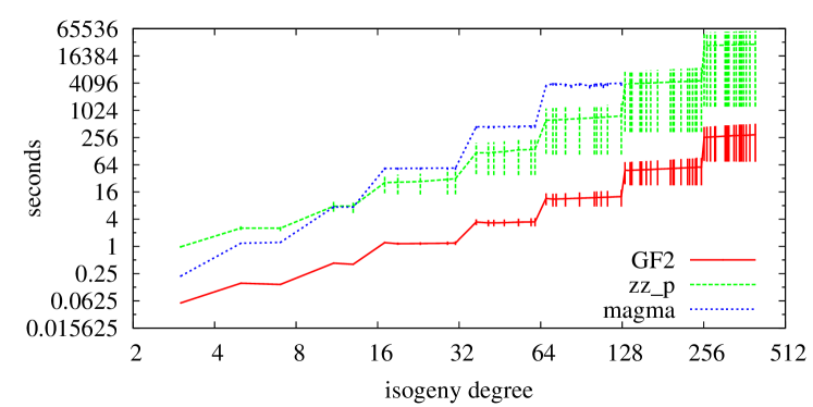
Figure 4: Comparative timings for different implementations of C2-AS-FI-MC with curves defined over $\mathbb{F}_{2^{101}}$. Plot in logarithmic scale.

The first set of experiments was run to evaluate the benefits of using the fast algorithms in [10]. We selected pairs of isogenous curves over $\mathbb{F}_{2^{101}}$ such that the height of the tower is maximal (observe that this is always the case for cryptographic curves). The library FAAST offers two types for finite field arithmetics in characteristic $2$: zz_p which is a generic type for word-precision $p$ and GF2 which uses the optimised algorithms of the library gf2x. We compared implementations of C2-AS-FI-MC using these two types with an implementation written in Magma. The results are in figure 4: we plot a line for the average running time of the algorithm and bars around it for minimum and maximum execution times of the final loop. Besides the dramatic speedup obtained by using the ad-hoc type GF2, the algorithmic improvements of FAAST over Magma are evident as even zz_p is one order of magnitude faster.

$\ell$	$E[p^{k}]$	$E^{\prime}[p^{k}]$	FI	RFR	MC	Avg tries	Avg loop time
31	1.3128	1.3128	1.1058	0.00218	0.00218	64	0.279
61	3.5454	3.5464	2.5236	0.00783	0.00900	128	2.154
127	9.2975	9.3026	5.6881	0.03147	0.03634	256	17.359
251	23.7984	23.7984	12.7251	0.12415	0.14519	512	137.902
397	59.7439	59.7579	28.3387	0.36822	0.58027	1024	971.254

Table 1: Comparative timings for the phases of C2-AS-FI-MC for curves over $\mathbb{F}_{2^{101}}$.

Table 1 shows detailed timings for each phase of C2-AS-FI-MC. The column FI reports the time for one interpolation, the column MC the time for one modular composition; comparing these two columns the gain from passing from C2-AS-FI to C2-AS-FI-MC is evident. Columns RFR (rational fraction reconstruction) and MC constitute the Cauchy interpolation step that is repeated in the final loop. The last column reports the average time spent in the loop: it is by far the most expensive phase and this justifies the attention we paid to FI and MC; only on some huge examples we approached the crosspoint between these two algorithms.

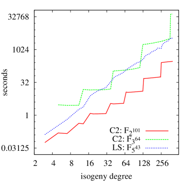
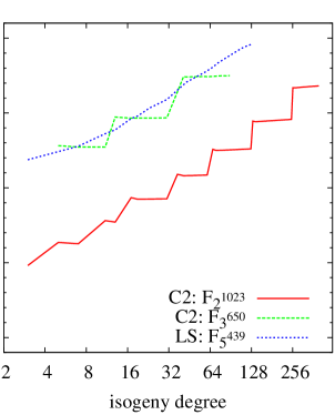
Figure 5: Comparative timings for C2-AS-FI-MC (C2) and LS over different curves. Plot in logarithmic scale.

Next, we compare the running times of C2-AS-FI-MC and LS over curves of half the cryptographic size in figure 5 (left). We only plot average times for C2, in characteristic $2$ we only plot the timings for GF2. From the plot it is clear that C2-AS-FI-MC only performs better than LS for $p=2$, but in this case the algorithm of [20] is by far better. Figure 5 (right) shows that LS slowly gets worse than C2, however comparing a Magma prototype to our highly optimised implementation of C2-AS-FI-MC is somewhat unfair and probably the crosspoint between the two algorithms lies much further. Furthermore, it is unlikely that C2-AS-FI-MC could be practical for any $p>3$ because of its high dependence on $p$, while LS scales pretty well with the characteristic as shown in figure 6.

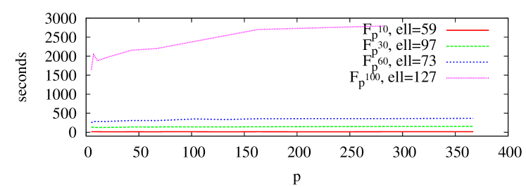
Figure 6: Timings for LS for different fields. We increase $p$ while taking constant $d$ and the isogeny degree.

We can hardly hide our disappointment concluding that, despite their good asymptotic behaviour and our hard work implementing them, the variants derived from C2 don’t seem to have any practical application, at least for present data sizes. We hope that in the future the algorithms presented here may turn useful to compute very large data that are currently out of reach.

References

- Atk [91] A.O.L. Atkin. The number of points on an elliptic curve modulo a prime. Email on the Number Theory Mailing List, 1991.
- BK [78] R.P. Brent and H.T. Kung, Fast algorithms for manipulating formal power series. J. ACM 25(4):581–595, 1978.
- BSS [99] I. Blake, G. Seroussi, and N. Smart. Elliptic curves in cryptography. Cambridge University Press, 1999.
- BMSS [08] A. Bostan, F. Morain, B. Salvy and É. Schost Fast algorithms for computing isogenies between elliptic curves. Math. Comp. 77, 263:1755-1778, 2008.
- [5] W. Bosma, J. Cannon, C. Playoust. The Magma algebra system. I. The user language. J. Symb. Comp., 24(3-4):235-265, 1997.
- [6] R. Brent, P. Gaudry, E. Thomé, P. Zimmermann. Faster multiplication in GF. In ANTS’08, 153–166. Springer, 2008.
- Cou [94] J.-M. Couveignes. Quelques calculs en théorie des nombres. PhD thesis. 1994.
- Cou [96] J.-M. Couveignes. Computing -isogenies using the -torsion. in ANTS’II, 59–65. Springer, 1996.
- Cou [00] J.-M. Couveignes. Isomorphisms between Artin-Schreier towers. Math. Comp. 69(232): 1625–1631, 2000.
- DFS [10] L. De Feo and É. Schost Fast Arithmetics in Artin Schreier Towers. Preprint, 2010.
- Elk [98] N.D. Elikes Elliptic and modular curves over finite fields and related computational issues. Computational Perspectives on Number Theory: Proceedings of a Conference in Honor of A.O.L. Atkin, 21–76, AMS, 1998.
- EM [03] A. Enge and F. Morain. Fast decomposition of polynomials with known Galois group. in AAECC-15, 254–264. Springer, 2003.
- JL [06] A. Joux, R. Lercier. Counting points on elliptic curves in medium characteristic. Cryptology ePrint Archive 2006/176, 2006.
- [14] J. von zur Gathen and J. Gerhard. Modern Computer Algebra. Cambridge University Press, 1999.
- vzGS [92] J. von zur Gathen and V. Shoup. Computing Frobenius maps and factoring polynomials Comput. Complexity, vol. 2, 187–224, 1992.
- Gun [76] H. Gunji. The Hasse Invariant and -division Points of an Elliptic Curve. Archiv der Mathematik 27(2), Springer, 1976.
- KS [97] E. Kaltofen and V. Shoup. Fast polynomial factorization over high algebraic extensions of finite fields. In ISSAC ’97, 184–188. ACM, 1997.
- KS [98] E. Kaltofen and V. Shoup. Subquadratic-time factoring of polynomials over finite fields. Math. Comput., 1179–1197, AMS, 1998.
- KU [08] K. S. Kedlaya and C. Umans Fast modular composition in any characteristic In FOCS’08, 146–155, IEEE, 2008
- Ler [96] R. Lercier. Computing isogenies in GF(). In ANTS-II, LNCS vol 1122, 197–212. Springer, 1996.
- Ler [97] R. Lercier. Algorithmique des courbes elliptiques dans les corps finis. Ph.D. Thesis, École polytechnique, 1997.
- LS [09] R. Lercier, T. Sirvent. On Elkies subgroups of -torsion points in curves defined over a finite field. To appear in J. Théor. Nombres Bordeaux.
- Mon [87] P. L. Montgomery Speeding the Pollard and Elliptic Curve Methods of Factorization Math. Comp., Vol. 48, No. 177., 243–264, 1987.
- RS [06] A. Rostovtsev and A. Stolbunov. Public-key cryptosystem based on isogenies. Cryptology ePrint Archive, Report 2006/145.
- Sat [00] T. Satoh. The canonical lift of an ordinary elliptic curve over a nite eld and its point counting. Journal of the Ramanujan Mathematical Society, 2000.
- Sch [95] R. Schoof. Counting points on elliptic curves over finite fields. J. Théorie des Nombres de Bordeaux 7:219–254, 1995.
- [27] V. Shoup. NTL: A library for doing number theory. http://www.shoup.net/ntl/.
- Tes [06] E. Teske. An elliptic trapdoor system. Journal of Cryptology, 19(1):115–133, 2006.
- Vél [71] J. Vélu. Isogénies entre courbes elliptiques. Comptes Rendus de l’Académie des Sciences de Paris 273, Série A, 238–241, 1971.
- Vol [90] J.F. Voloch. Explicit -descent for Elliptic Curves in Characteristic . Compositio Mathematica 74, 247–58, 1990.