Classical Statistical Mechanics Approach to Multipartite Entanglement

Abstract

We characterize the multipartite entanglement of a system of $n$ qubits in terms of the distribution function of the bipartite purity over balanced bipartitions. We search for maximally multipartite entangled states, whose average purity is minimal, and recast this optimization problem into a problem of statistical mechanics, by introducing a cost function, a fictitious temperature and a partition function. By investigating the high-temperature expansion, we obtain the first three moments of the distribution. We find that the problem exhibits frustration.

1 Introduction

There is a profound diversity between quantum mechanical and classical correlations. Schrödinger [1, 2] coined the term “entanglement” to describe the peculiar connection that can exist between quantum systems, that was first perceived by Einstein, Podolsky and Rosen [3] and has no analogue in classical physics. Entanglement is a resource in quantum information science [4, 5, 6] and is at the origin of many unique quantum phenomena and applications, such as superdense coding [7], teleportation [8] and quantum cryptographic schemes [9, 10, 11, 12].

Much progress has been made in developing a quantitative theory of entanglement [5, 6]. The bipartite entanglement between simple systems can be unambiguously defined in terms of the von Neumann entropy or the entanglement of formation [13, 4, 14]. On the other hand, an exhaustive characterization of multipartite entanglement is more elusive [5, 6] and different definitions [15, 16, 17, 18, 19] often do not agree with each other, essentially because they tend to capture different aspects of the phenomenon. More to this, a complete evaluation of global entanglement measures bears serious computational difficulties, because states endowed with large entanglement typically involve exponentially many coefficients.

We proposed in [20] that multipartite entanglement shares many characteristic traits of complex systems and can therefore be analyzed in terms of the probability density function of an entanglement measure (say purity) of a subsystem over all (balanced) bipartitions of the total system [21]. A state has a large multipartite entanglement if its average bipartite entanglement is large. In addition, if the entanglement distribution has a small standard deviation, bipartite entanglement is essentially independent of the bipartition and can be considered as being fairly “shared” among the elementary constituents (qubits) of the system. Clearly, average and standard deviation are but the first two moments of a distribution function. A full characterization of the multipartite entanglement of a quantum state must therefore take into account higher moments and/or the whole distribution function, in particular if the latter is not bell shaped or is endowed with unusual and/or irregular features.

The idea that complicated phenomena cannot be summarized in a single (or a few) number(s), but rather require a large number of measures (or even a whole function) is not novel in the context of complex systems [22] and even in the study of quantum entanglement [23]. In this article we shall pursue this idea even further and shall study the bipartite and multipartite entanglement of a system of qubits by making full use of the tools and techniques of classical statistical mechanics: we shall explore the features of a partition function, expressed in terms of the average purity of a subset of the qubits: this will be viewed as a cost function, that plays the role of the Hamiltonian. Interestingly, this approach brings to light the presence of frustration in the system [24], highlighting the complexity inherent in the phenomenon of multipartite entanglement.

This paper is organized as follows. We introduce notation and define maximally bipartite and maximally multipartite entangled states in Sec. 2. Multipartite entanglement is characterized in terms of the distribution function of bipartite entanglement in Sec. 3. The statistical mechanical approach and the partition function are introduced in Sec. 4. The high temperature expansion and its first three cumulants are computed in Sec. 5. Section 6 contains our conclusions and an outlook.

2 From bipartite to multipartite entanglement

2.1 Bipartite purity

We consider an ensemble $S=\{1,2,\dots,n\}$ of $n$ qubits in the Hilbert space $\mathcal{H}_{S}=(\mathbb{C}^{2})^{\otimes n}$ and focus on pure states

$$|\psi\rangle=\sum_{k\in{\mathbb{Z}}_{2}^{n}}z_{k}|k\rangle,\quad z_{k}\in\mathbb{C},\quad\sum_{k\in{\mathbb{Z}}_{2}^{n}}{|z_{k}|}^{2}=1,$$ (1)

where $k=(k_{i})_{i\in S}$, with $k_{i}\in{\mathbb{Z}}_{2}=\{0,1\}$, and

$$|k\rangle=\bigotimes_{i\in S}|k_{i}\rangle_{i},\qquad|k_{i}\rangle_{i}\in\mathbb{C}^{2},\qquad\langle k_{i}|k_{j}\rangle=\delta_{ij}.$$ (2)

For the sake of simplicity, in this paper we shall focus on pure states of qubits and shall not discuss additional phenomena such as bound entanglement [25, 26]. Consider a bipartition $(A,\bar{A})$ of the system, where $A\subset S$ is a subset of $n_{A}$ qubits and $\bar{A}=S\backslash A$ its complement, with $n_{A}+n_{\bar{A}}=n$. We set $n_{A}\leq n_{\bar{A}}$ with no loss of generality. The total Hilbert space factorizes into $\mathcal{H}_{S}=\mathcal{H}_{A}\otimes\mathcal{H}_{\bar{A}}$, with $\mathcal{H}_{A}=\bigotimes_{i\in A}\mathbb{C}^{2}_{i}$, of dimensions $N_{A}=2^{n_{A}}$ and $N_{\bar{A}}=2^{n_{\bar{A}}}$, respectively ($N_{A}N_{\bar{A}}=N$). As a measure of the bipartite entanglement between the two subsets, we consider the purity of subsystem $A$

$$\pi_{A}=\tr_{A}\rho_{A}^{2},\quad\rho_{A}=\tr_{\bar{A}}|\psi\rangle\langle\psi|,$$ (3)

$\tr_{X}$ being the partial trace over $X=A$ or $\bar{A}$. We notice that $\pi_{A}=\pi_{\bar{A}}$ and

$$1/N_{A}\leq\pi_{A}\leq 1.$$ (4)

State (1) can be written according to the bipartition $(A,\bar{A})$ as

$$|\psi\rangle=\sum_{k\in{\mathbb{Z}}_{2}^{n}}z_{k}|k_{A}\rangle_{A}\otimes|k_{\bar{A}}\rangle_{\bar{A}},$$ (5)

where $k_{A}=(k_{i})_{i\in A}$ and $|l\rangle_{A}=\bigotimes_{i\in A}|l_{i}\rangle_{i}\in\mathcal{H}_{A}$. By plugging Eq. (5) into Eq. (3) we obtain

$$\rho_{A}=\sum_{k,l\in{\mathbb{Z}}_{2}^{n}}z_{k}\bar{z}_{l}\delta_{k_{\bar{A}},l_{\bar{A}}}|k_{A}\rangle\langle l_{A}|$$ (6)

and

$$\pi_{A}=\sum_{k,k^{\prime},l,l^{\prime}\in{\mathbb{Z}}_{2}^{n}}z_{k}z_{k^{\prime}}\bar{z}_{l}\bar{z}_{l^{\prime}}\delta_{k_{A},l^{\prime}_{A}}\delta_{k^{\prime}_{A},l_{A}}\delta_{k_{\bar{A}},l_{\bar{A}}}\delta_{k^{\prime}_{\bar{A}},l^{\prime}_{\bar{A}}},$$ (7)

which is a quartic function of the coefficients of the expansion (1). If, for example, the system is partitioned into two blocks of contiguous qubits $(C,\bar{C})$, namely $C=\{1,2,\dots,n_{A}\}$, then

$$\pi_{C}=\sum_{l,l^{\prime}\in{\mathbb{Z}}_{2}^{n_{A}}}\sum_{m,m^{\prime}\in{\mathbb{Z}}_{2}^{n_{\bar{A}}}}z_{(l,m)}\bar{z}_{(l^{\prime},m)}z_{(l^{\prime},m^{\prime})}\bar{z}_{(l,m^{\prime})},$$ (8)

where $(l,m)=(l_{1},\dots,l_{n_{A}},m_{1},\dots,m_{n_{\bar{A}}})\in{\mathbb{Z}}_{2}^{n}$.

2.2 Minimal bipartite purity

For a given bipartition it is very easy to saturate the lower bound $1/N_{A}$ of (7). For example,

$$z_{k}=N_{A}^{-1/2}\delta_{k_{A},k_{\bar{A}}},$$ (9)

which represents a maximally bipartite entangled state

$$|\psi\rangle=N_{A}^{-1/2}\sum_{l\in{\mathbb{Z}}_{2}^{n_{A}}}|l\rangle_{A}\otimes|l\rangle_{\bar{A}},$$ (10)

yields $\rho_{A}=\mathbf{1}/N_{A}$ and $\pi_{A}=1/N_{A}$. In fact, the general minimizer is a maximally bipartite entangled state whose Schmidt basis is not the computational basis, namely,

$$z_{k}=N_{A}^{-1/2}\sum_{l\in{\mathbb{Z}}_{2}^{n_{A}}}U^{A}_{k_{A},l}U^{\bar{A}}_{k_{\bar{A}},l},$$ (11)

where $U^{A}_{l,l^{\prime}}=\langle l_{A}|U^{A}|l^{\prime}_{A}\rangle$ with $U^{A}$ a local unitary operator in $\mathcal{H}_{A}$ that transforms the computational bases into the Schmidt one, that is

$$|\psi\rangle=N_{A}^{-1/2}\sum_{l\in{\mathbb{Z}}_{2}^{n_{A}}}U^{A}|l\rangle_{A}\otimes U^{\bar{A}}|l\rangle_{\bar{A}}.$$ (12)

For this state, $\pi_{A}(|\psi\rangle)=1/N_{A}$. The information contained in a maximally bipartite entangled state with $n_{A}=n_{\bar{A}}$ is not locally accessible by party $A$ or $\bar{A}$, because their partial density matrices are maximally mixed, but rather is totally shared by them.

2.3 Average purity and MMES

Entanglement, in very few words, embodies the impossibility of factorizing a state of the total quantum system in terms of the states of its constituents. Most measures of bipartite entanglement (for pure states) exploit the fact that when a (pure) quantum state is entangled, its constituents do not have (pure) states of their own. This is, for instance, what we did in the previous section. We wish to generalize the above distinctive trait to the case of multipartite entanglement, by requiring that this feature be valid for all bipartitions.

Let $|\psi\rangle\in\mathcal{H}_{S}$ and consider the average purity [27, 29]

$$\pi_{\mathrm{ME}}^{(n)}(|\psi\rangle)=\mathbb{E}[\pi_{A}]=\left(\begin{array}[]{l}n\\ n_{A}\end{array}\!\!\right)^{-1}\sum_{|A|=n_{A}}\pi_{A},$$ (13)

where $\mathbb{E}$ denotes the expectation value, $|A|$ is the cardinality of $A$ and the sum is over balanced bipartitions $n_{A}=[n/2]$, where $[x]$ denotes the integer part of $x$. Since we are focusing on balanced bipartitions, and any bipartition can be brought into any other bipartition by applying a permutation of the qubits, the sum over balanced bipartitions in (13) is equivalent to a sum over the permutations of the qubits. The quantity $\pi_{\mathrm{ME}}$ measures the average bipartite entanglement over all possible balanced bipartitions and inherits the bounds (4)

$$1/N_{A}\leq\pi_{\mathrm{ME}}^{(n)}(|\psi\rangle)\leq 1.$$ (14)

The average purity introduced in Eq. (13) is related to the average linear entropy $S_{L}=\frac{N_{A}}{N_{A}-1}(1-\pi_{\mathrm{ME}})$ [27] and extends ideas put forward in [18, 28].

A maximally multipartite entangled state (MMES) [29] $|\varphi\rangle$ is a minimizer of $\pi_{\mathrm{ME}}$,

$$\pi_{\mathrm{ME}}^{(n)}(|\varphi\rangle)=E_{0}^{(n)},$$ (15)

$$\mathrm{with}\quad E_{0}^{(n)}=\min\{\pi_{\mathrm{ME}}^{(n)}(|\psi\rangle)\;|\;|\psi\rangle\in\mathcal{H}_{S},\langle\psi|\psi\rangle=1\}.$$

The meaning of this definition is clear: the density matrix of each subsystem $A\subset S$ of a MESS is as mixed as possible (given the constraint that the total system is in a pure state), so that the information contained in a MMES is as distributed as possible.

2.4 Perfect MMES and the symptoms of frustration

For small values of $n$ one can tackle the minimization problem (15) both analytically and numerically. For $n=2,3,5,6$ the average purity saturates its minimum in (14): this means that purity is minimal for all balanced bipartitions. In this case we shall say that the MMES is perfect.

For $n=2$ (perfect) MMES are Bell states up to local unitary transformations, while for $n=3$ they are equivalent to the GHZ states [30]. For $n=4$ one numerically obtains $E_{0}^{(4)}=\min\pi_{\mathrm{ME}}^{(4)}=1/3>1/4=1/N_{A}$ [29, 31, 32, 33]. For $n=5$ and 6 one can find several examples of perfect MESS, some of which can be expressed in terms of binary strings of coefficients [$z_{k}=\pm 1$ in Eq. (1)].

The case $n=7$ is still open, our best estimate being $E_{0}^{(7)}\simeq 0.13387>1/8=1/N_{A}$. Most interestingly, perfect MMES do not exist for $n\geq 8$ [27]. These findings are summarized in Table 1. This brings to light an intriguing feature of multipartite entanglement: we observed in Sec. 2.2 that it is always possible to saturate the lower bound in (4)

$$\pi_{A}^{(n)}=1/N_{A}$$ (16)

for a given bipartition $(A,\bar{A})$. However, in order to saturate the lower bound

$$E_{0}^{(n)}=1/N_{A}$$ (17)

in Eq. (14), it must happen that (16) be valid for any bipartition in the average (13). As we have seen, this requirement can be satisfied only for very few “special” values of $n$. For all other values of $n$ this is impossible: different bipartitions “compete” with each other, and the minimum $E_{0}^{(n)}$ of $\pi_{\mathrm{ME}}^{(n)}$ is strictly larger than $1/N_{A}$. We view this “competition” among different bipartitions as a phenomenon of frustration: it is already present for $n$ as small as 4 [24]. (Interestingly, an analogous phenomenon exists also for “Gaussian MMES”, see [34].)

This frustration is the main reason for the difficulties one encounters in minimizing $\pi_{\mathrm{ME}}$ in (13). Notice that the dimension of $\mathcal{H}_{S}$ is $N=2^{n}$ and the number of partitions scales like $2^{N}$. We therefore need to define a viable strategy for the characterization of MMES, when $n\geq 8$.

Table 1: Perfect MMES for different number $n$ of qubits.

$n$	perfect MMES
2,3	exist
4	do not exist
5,6	exist
7	?
$\geq 8$	do not exist

3 Probability distribution of bipartite entanglement

We now introduce the distribution function of purity over all bipartitions, $p(\pi_{A})$, that will induce a probability-density-function characterization of multipartite entanglement. For rather regular (i.e. bell-shaped) distributions the first few moments already yield a good characterization: in particular, the average will measure the amount of entanglement of the state when the bipartitions are varied, while the variance will quantify how uniformly is bipartite entanglement distributed among balanced bipartitions.

The calculation of the properties of $\pi_{A}$ is particularly simple for an important class of states. Consider the set

$$C=\left\{(z_{1},z_{2},\ldots,z_{N})\in\mathbb{C}^{N}|\sum_{k}|z_{k}|^{2}=1\right\},$$ (18)

corresponding to normalized vectors in $\mathcal{H}_{S}$. This set is left invariant under the natural action of the unitary group $\mathcal{U}(\mathcal{H}_{S})$. A typical state is obtained by sampling with respect to the action of $\mathcal{U}(\mathcal{H}_{S})$ on this set. Typical states have been extensively studied in the literature [35, 36, 37, 38, 39, 40] and can be (efficiently) generated by a chaotic dynamics [41, 42].

For large $N$, the $\pi_{A}$’s have a bell-shaped distribution over the bipartitions with mean and variance [21]

$$\mu^{(n)} = \langle\pi_{A}\rangle_{0}=\frac{N_{A}+N_{\bar{A}}}{N+1},$$ (19)

$$\sigma^{2} = \langle(\pi_{A}-\mu)^{2}\rangle_{0}=\frac{2(N_{A}^{2}-1)(N_{\bar{A}}^{2}-1)}{(N+1)^{2}(N+2)(N+3)},$$ (20)

respectively, where the brackets $\langle\cdots\rangle_{0}$ denote the average with respect to the unitarily invariant measure over pure states

$$\mathrm{d}\mu_{C}(z)=\frac{(N-1)!}{\pi^{N}}\;\delta\!\left(1-\sum_{k}|z_{k}|^{2}\right)\prod_{k}{\mathrm{d}z_{k}\mathrm{d}\bar{z}_{k}},$$ (21)

induced by the Haar measure over $\mathcal{U}(\mathcal{H_{S}})$ through the mapping $|\psi\rangle=\sum z_{j}|j\rangle=U|\psi_{0}\rangle$, for a given reference state $|\psi_{0}\rangle$ [38]. Here $\mathrm{d}z_{k}\mathrm{d}\bar{z}_{k}=\mathrm{d}x_{k}\mathrm{d}y_{k}$, with $x_{k}=\mathop{\mathrm{Re}}\nolimits z_{k}$ and $y_{k}=\mathop{\mathrm{Im}}\nolimits z_{k}$, denotes the Lesbegue measure on $\mathbb{C}$.

Given a state $|\psi\rangle\in\mathcal{H}_{S}$, the potential of multipartite entanglement has the following expression in terms of its Fourier coefficients $z_{i}$

$$\pi_{\mathrm{ME}}=\sum_{k,k^{\prime},l,l^{\prime}\in{\mathbb{Z}}_{2}^{n}}\Delta(k,k^{\prime};l,l^{\prime})\,z_{k}\,z_{k^{\prime}}\,\bar{z}_{l}\,\bar{z}_{l^{\prime}}\,,$$ (22)

with a coupling function

$$\quad\Delta(k,k^{\prime};l,l^{\prime})=\left(\!\!\begin{array}[]{c}n\\ n_{A}\end{array}\!\!\right)^{\!\!-1}\!\!\!\sum_{|A|=n_{A}}\!\frac{1}{2}\left(\delta_{k_{A},l^{\prime}_{A}}\delta_{k^{\prime}_{A},l_{A}}\delta_{k_{\bar{A}},l_{\bar{A}}}\delta_{k^{\prime}_{\bar{A}},l^{\prime}_{\bar{A}}}+\delta_{k^{\prime}_{A},l^{\prime}_{A}}\delta_{k_{A},l_{A}}\delta_{k^{\prime}_{\bar{A}},l_{\bar{A}}}\delta_{k_{\bar{A}},l^{\prime}_{\bar{A}}}\right),$$ (23)

with $n_{A}=[n/2]$ (balanced bipartitions). The result follows by plugging the expression (7) of $\pi_{A}$ into Eq. (13), and by symmetrizing under the exchange $k\leftrightarrow k^{\prime}$ (or, equivalently, $A\leftrightarrow\bar{A}$). The coupling function $\Delta$ has the following expression (see A for details)

$$\Delta(k,k^{\prime};l,l^{\prime})=g\big{(}(k\oplus l)\vee(k^{\prime}\oplus l^{\prime}),(k\oplus l^{\prime})\vee(k^{\prime}\oplus l)\big{)},$$ (24)

where

$$g(a,b)=\delta_{a\wedge b,\,0}\;\hat{g}(|a|,|b|),$$ (25)

with $|a|=\sum_{i\in S}a_{i}$, $|b|=\sum_{i\in S}b_{i}$, $a\oplus b=(a_{i}+b_{i}\;\mathrm{mod}\;2)_{i\in S}$ is the XOR operation, $a\vee b=(a_{i}+b_{i}-a_{i}b_{i})_{i\in S}$ the OR operation, $a\wedge b=(a_{i}b_{i})_{i\in S}$ the AND operation and

$$\hat{g}(s,t)=\frac{1}{2}\left(\!\!\begin{array}[]{c}n\\ {n_{A}}\end{array}\!\!\right)^{\!\!-1}\left[\left(\!\!\begin{array}[]{c}n-s-t\\ {n_{A}}-s\end{array}\!\!\right)+\left(\!\!\begin{array}[]{c}n-s-t\\ {n_{A}}-t\end{array}\!\!\right)\right].$$ (32)

Using the definitions we notice the following symmetries of the coupling function:

$$\left\{\begin{array}[]{c}\Delta(k,k^{\prime};l,l^{\prime})=\Delta(k^{\prime},k;l,l^{\prime})\\ \Delta(k,k^{\prime};l,l^{\prime})=\Delta(l,l^{\prime};k,k^{\prime})\\ \Delta(k,k^{\prime};l,l^{\prime})=\Delta(k^{\prime},k;l^{\prime},l)\end{array}\right..$$ (36)

4 Partition function

In order to study the minimization problem, we will reformulate it in terms of classical statistical mechanics: in particular, the minimum $E_{0}$ of $\pi_{\mathrm{ME}}$ will be recovered in the zero temperature limit of a suitable classical system.

The main quantity we are interested in is the average bipartite entanglement between balanced bipartitions, $\pi_{\mathrm{ME}}$ in Eq. (13). This quantity will play the role of energy in the statistical mechanical approach. We therefore start by viewing $\pi_{\mathrm{ME}}$ in Eq. (13) as a cost function (potential of multipartite entanglement) and write

$$H(z)=\pi_{\mathrm{ME}}(|\psi\rangle),$$ (37)

where $z$ are the Fourier coefficients of the expansion (1). We consider an ensemble $\{m_{j}\}$ of $M$ vectors (states), where $m_{j}$ is the number of vectors with purity $H=\epsilon_{j}$. In the standard ensemble approach to statistical mechanics one seeks the distribution that maximizes the number of states $\Omega=M!/\prod_{j}m_{j}!$ under the constraints that $\sum_{j}m_{j}=M$ and $\sum_{j}m_{j}\epsilon_{j}=ME$. For $M\to\infty$, the above optimization problem yields the canonical ensemble and its partition function

$$\qquad Z(\beta)=\int\mathrm{d}\mu_{C}(z)\mathrm{e}^{-\beta H(z)}=c_{N}\int\mathrm{d}\mu_{\mathrm{H}}(U)\exp\left(-\beta\mathbb{E}[\tr_{A}(\tr_{\bar{A}}U|\psi_{0}\rangle\langle\psi_{0}|U^{\dagger})^{2}]\right),$$ (38)

where the expectation value $\mathbb{E}$ was introduced in Eq. (13) and the Lagrange multiplier $\beta$, that plays the role of an inverse temperature, fixes the average value of purity $E$. In the first integral we have used the measure (21) and taken into account the normalization condition (18). In the last (base-independent) expression $\mu_{\mathrm{H}}$ denotes the Haar measure over $\mathcal{U}(\mathcal{H})$, $|\psi_{0}\rangle$ is any given vector and the (unimportant) constant $c_{N}$ is proportional to the ratio $\mu_{C}(\mathbb{C}^{N})/\mu_{\mathrm{H}}(\mathcal{U}(\mathcal{H}))$ between the area of the $(N-1)$-dimensional sphere (18) and the volume of the unitary group. In conclusion, the potential of multipartite entanglement can be now considered as the Hamiltonian of a classical statistical mechanical system.

4.1 Comments

In order to clarify the rationale behind our analysis, a few comments are necessary.

i) Although our interest is focused on the microcanonical features of the system, namely on “isoentangled” manifolds [43], we find it convenient to define a canonical ensemble and a temperature. This makes the analysis easier to handle and is at the very foundations of statistical mechanics, when one discusses the equivalence in the description of large systems between the microcanonical ensemble (in which energy is fixed) and the canonical ensemble (in which temperature is fixed).

ii) One can view the multipartite system as an ensemble for the collection of all balanced bipartitions. However, what makes the problem intricate and interesting is the fact that there is a nontrivial interaction among different bipartitions, which in general provokes frustration.

iii) From a physical point of view, the measure of typical states is a uniform measure over the whole projective space. This would be consistent with ergodicity. However, our analysis is purely static and we are not considering the time evolution generated by the (purity) Hamiltonian. The relaxation to equilibrium, as well as its ergodic properties, deserve a deeper study and would probably uncover additional features with respect to the equilibrium situation. This aspect will be investigated in the future.

iv) Temperature is a Lagrange multiplier for the optimization parameter. It is the variable that is naturally conjugate to $H$, in exactly the same way as inverse temperature is conjugate to energy: $\beta$ fixes, with an uncertainty that becomes smaller for a larger system, the level of the purity of the subset of vectors under consideration, and thus an isoentangled submanifold. The use of a temperature is a common expedient in problems that can be recast in terms of classical statistical mechanics. One can find examples of this kind in the stochastic approach to optimization processes (for instance simulated annealing) [44, 45].

4.2 Some limits

We start by looking at some interesting limits and give a few preliminary remarks. For $\beta\to 0$, Eq. (38) clearly yields the distribution of the typical states (21). For $\beta\to+\infty\;(T\to 0^{+})$, only those configurations that minimize the Hamiltonian survive, namely the MMES. There is a physically appealing interpretation even for negative temperatures: for $\beta\to-\infty\;(T\to 0^{-})$, those configurations are selected that maximize the Hamiltonian, that is separable (factorized and non-entangled) states.

The energy distribution function at arbitrary $\beta$ can be obtained from the partition function

$$Z(\beta) = \int\mathrm{d}\mu_{C}(z)\mathrm{e}^{-\beta H(z)}=\int_{E_{0}}^{1}\mathrm{d}E\mathrm{e}^{-\beta E}\int\mathrm{d}\mu_{C}(z)\,\delta(H(z)-E),$$ (39)

where $E\in[E_{0},1]$, $E_{0}$ being the minimum of the spectrum of $H$ and $\delta$ the Dirac function. Incidentally, notice that Eqs. (14) and (19) yield

$$\lim_{n\to\infty}E_{0}^{(n)}\leq\lim_{n\to\infty}\mu^{(n)}=0,\qquad E_{0}^{(n)}\geq 2^{-[n/2]},\quad\mu^{(n)}=\frac{2^{[n/2]}+2^{[(n+1)/2]}}{2^{n}+1}.$$

The energy distribution function reads

$$P_{\beta}(E) = \frac{\mathrm{e}^{-\beta E}}{Z(\beta)}\int\mathrm{d}\mu_{C}(z)\,\delta(H(z)-E)$$ (41)

which, for $\beta=0$, simply reads

$$P_{0}(E) = \frac{1}{Z(0)}\int\mathrm{d}\mu_{C}(z)\,\delta(H(z)-E).$$ (42)

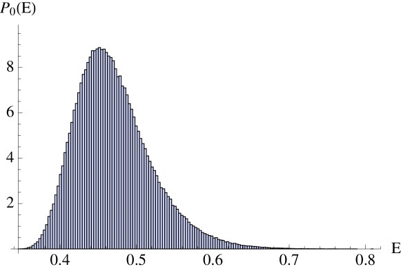
Figure 1: (Color online) Probability density function $P_{0}(E)$ for $n=4$. The distribution has been obtained from $5\times 10^{5}$ typical states. The binning is $3\times 10^{-3}$ and the integral is equal to $1$.

In Fig. 1 we show the probability density function $P_{0}(E)$ for $n=4$. As emphasized in Sec. 2.4, this is one of those cases in which frustration appears, as for $n=4$ qubits one (numerically) finds $E_{0}^{(4)}=\min\pi_{\mathrm{ME}}^{(4)}=1/3>1/4=1/N_{A}$ [29, 31, 32, 33]. We clearly observe the asymmetry of the curve, denoting a positive value of the skewness. This deformation becomes less evident for larger values of $n$. As we will see, in the thermodynamic limit, $n\to\infty$, $P_{0}(E)$ will become more and more symmetric and will tend to a Gaussian.

Using Eqs. (39)-(42) we obtain the expression of the energy distribution function at arbitrary $\beta$ in terms of its infinite temperature limit:

$$P_{\beta}(E)=\frac{\mathrm{e}^{-\beta E}P_{0}(E)}{\int_{E_{0}}^{1}\mathrm{d}E\,\mathrm{e}^{-\beta E}P_{0}(E)}.$$ (43)

Notice that this equation is valid at fixed $n$.

By multiplying and dividing the last equation by $|\beta|\mathrm{e}^{\beta}$ and $\beta\mathrm{e}^{\beta E_{0}}$, respectively, and remembering that

$$\frac{1}{\epsilon}\,\mathrm{e}^{-x/\epsilon}\stackrel{{\scriptstyle\epsilon\rightarrow 0}}{{\longrightarrow}}\delta(x)$$ (44)

we find

$$P_{-\infty}(E)=\delta(E-1),\qquad P_{\infty}(E)=\delta(E-E_{0}).$$ (45)

These limits are the counterparts of those discussed for the partition function and are reflected in the asymptotic behaviour of the average energy as function of $\beta$

$$\langle H\rangle_{\beta}=\frac{1}{Z(\beta)}\int\mathrm{d}\mu_{C}(z)H\mathrm{e}^{-\beta H}=\int_{E_{0}}^{1}\mathrm{d}E\,EP_{\beta}(E)=-\frac{\partial}{\partial\beta}\ln Z(\beta).$$ (46)

Indeed,

$$\langle H\rangle_{\beta\to-\infty}=1,\quad\langle H\rangle_{\beta\to+\infty}=E_{0}.$$ (47)

More generally, the $m$-th cumulant of $H$ reads

$$\kappa^{(m)}_{\beta}[H]={(-)}^{m}\frac{\partial^{m}}{\partial{\beta}^{m}}\ln Z(\beta)={(-)}^{m-1}\frac{\partial^{m-1}}{\partial{\beta}^{m-1}}\langle H\rangle_{\beta}.$$ (48)

We find

$$\frac{\partial}{\partial\beta}\langle H\rangle_{\beta}=-\kappa^{(2)}_{\beta}[H]=-\langle H^{2}\rangle_{\beta}+\langle H\rangle_{\beta}^{2}\equiv-\bar{\sigma}^{2}_{\beta}\leqslant 0,$$ (49)

which is non-positive. In particular

$$\bar{\sigma}^{2}=\bar{\sigma}^{2}_{0}=\kappa^{(2)}_{0}[H].$$ (50)

The average energy is a non-increasing function of $\beta$ and has at least one inflexion point as function of $\beta$. Moreover

$$\kappa^{(3)}_{\beta}[H]=\frac{\partial^{2}}{\partial\beta^{2}}\langle H\rangle_{\beta}=-\frac{1}{2}\frac{\partial}{\partial\beta}\bar{\sigma}^{2}_{\beta}.$$ (51)

From the qualitative behaviour of $\kappa^{3}_{\beta}$ one can obtain information about the width of the distribution. For $\beta\to+\infty$ the curvature of $\langle H\rangle_{\beta}$ is positive and therefore $\bar{\sigma}^{2}_{\beta}$ is a decreasing function.

From a qualitative point of view, one expects the behavior sketched in Fig. 2: for $\beta\to 0^{+}\;(T\to+\infty)$, the distribution is bell-shaped (typical states); when $\beta\to+\infty\;(T\to 0^{+})$ the distribution tends to become more concentrated around $E_{0}$. The energy distribution (43) at sufficiently high temperatures [how high will be discussed in Sec. 5.4, see Eq. (164)] can be obtained by observing that from Eq. (49)

$$P_{\beta}(E)\sim P_{0}(E+\beta\bar{\sigma}^{2}).$$ (52)

For larger values of $\beta$ the left tail of the distribution starts “feeling” the wall at $E_{0}$. The value of $P_{0}(E_{0})$ influences the behaviour of $P_{\beta}(E)$. In general, $P_{0}(E_{0})$ can vanish or not, yielding the behavior sketched in Fig. 2(a) and (b), respectively. One finds

$$P_{\beta}(E)\sim\frac{\beta^{r+1}}{r!}(E-E_{0})^{r}\mathrm{e}^{-\beta(E-E_{0})},$$ (53)

where $r$ is the order of the first nonvanishing derivative of $P_{0}(E)$ at $E_{0}$. [Figs. 2(a), (b) display the case $r=0,1$, respectively] Notice that the only relic of $P_{0}(E)$ in (53) is $r$ and $P_{\beta\to\infty}(E)$ yields the second equation in (45). Actually if $r=0$, Eq. (53) yields a pure exponential converging to

$$P_{+\infty}(E)=\delta(E-E_{0}).$$ (54)

If $r\geq 1$ the probability for finite $\beta$ has an initial polynomial increase but still converges to a Dirac $\delta$ in $E_{0}$, corresponding to MMESs. The analysis for $\beta\to-\infty$ is analogous (we expand $P_{\beta}(E)$ around $E=1$, which is the maximum of $H$); it yields the first equation in (45). In this limit we obtain the separable states.

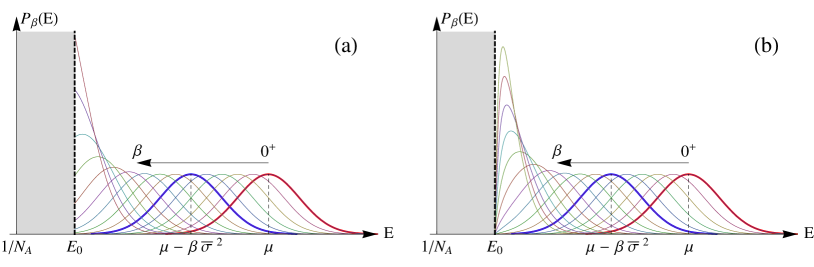
Figure 2: (Color online) Qualitative sketch of Eq. (43), at fixed $N_{A}$, in arbitrary units. The energy density function is distributed around $\mu$ with standard deviation $\bar{\sigma}$ at $\beta=0$ (first bell-shaped curve at the right in both panels) and moves toward $E_{0}$ when $\beta$ increases. In each panel, from right to left, $\beta$ changes in constant steps. The probability density rigidly shifts with $\beta$, for $\beta\lesssim N^{7/2-\log_{2}3}$: see Eq. (163) and following discussion. Note that both $E_{0},\mu$ are $O(N^{-1/2})$. In (a) $P_{0}(E_{0})\neq 0$; in (b) $P_{0}(E_{0})=0$.

5 High temperature expansion

This section is devoted to the study of the cumulants of $P_{0}(E)$. This will enable us to look at some properties of the high temperature expansion of the distribution function of the potential of multipartite entanglement. We remind that for $\beta\to 0$ one gets the typical states.

The high temperature expansion originates from the Taylor series

$$\kappa^{(m)}_{\beta}[H] = {(-)}^{m}\left.\sum_{j=0}^{\infty}\frac{\beta^{j}}{j!}\left(\frac{\partial^{m+j}}{\partial\beta^{m+j}}\ln Z(\beta)\right)\right|_{\beta=0}$$ (55)

$$= \sum_{j=0}^{\infty}\frac{{(-\beta)}^{j}}{j!}\kappa^{(m+j)}_{\beta=0}[H].$$

The average energy reads

$$\langle H\rangle_{\beta} = \sum_{m=1}^{\infty}\frac{(-\beta)^{m-1}}{(m-1)!}\kappa_{\beta=0}^{(m)}[H]$$ (56)

$$\sim \langle H\rangle_{0}-\beta\left\langle{\left(H-\langle H\rangle_{0}\right)}^{2}\right\rangle_{0}+\frac{\beta^{2}}{2}\left\langle{\left(H-\langle H\rangle_{0}\right)}^{3}\right\rangle_{0},$$

while the free energy takes the form

$$F(\beta) = \frac{1}{\beta}\ln Z(\beta)$$ (57)

$$\sim \frac{\ln Z(0)}{\beta}-\langle H\rangle_{0}+\frac{\beta}{2}\left\langle{\left(H-\langle H\rangle_{0}\right)}^{2}\right\rangle_{0}-\frac{\beta^{2}}{6}\left\langle{\left(H-\langle H\rangle_{0}\right)}^{3}\right\rangle_{0}.$$

In the following three subsections we will evaluate the first three cumulants of the distribution for $\beta=0$ in order to characterize the high temperature expansion of the energy distribution function.

5.1 First cumulant

The joint probability density of $z=(z_{k})\in\mathbb{C}^{N}$ associated to the measure of typical states (21) is

$$p_{N}(z_{1},z_{2},\dots,z_{N})=\frac{(N-1)!}{\pi^{N}}\;\delta\!\left(1-\sum_{1\leq k\leq N}|z_{k}|^{2}\right).$$ (58)

By integrating out $N-M$ variables, one gets

$$p_{N}(z_{1},z_{2},\dots,z_{M})=\frac{(N-1)!}{(N-M-1)!\;\pi^{M}}\,\left(1-\sum_{1\leq k\leq M}|z_{k}|^{2}\right)^{N-M-1},$$ (59)

for $1\leq M<N$. In particular the probability density of an arbitrary element of $z$ is

$$p_{N}(z_{1})=\frac{N-1}{\pi}\;(1-|z_{1}|^{2})^{N-2}.$$ (60)

Since $\langle e^{i\arg z_{j}}\rangle_{0}=0$, the only nonvanishing averages of the type

$$\left\langle\prod_{k\in X}z_{k}\prod_{l\in Y}\bar{z}_{l}\right\rangle_{0},$$ (61)

with $X,Y\subset{\mathbb{Z}}_{2}^{n}$, are obtained when the variables $\{z_{k}\}$ and $\{\bar{z}_{l}\}$ are equal pair by pair, that is when the sets of indices are equal, $X=Y$. The nonvanishing correlation functions are given by

$$\left\langle\prod_{j=1}^{k}|z_{q_{j}}|^{2m_{j}}\right\rangle_{0} = \int\prod_{j=1}^{k}|z_{j}|^{2m_{j}}p_{N}(z_{1},\dots,z_{N})\prod_{j}dz_{j}d\bar{z}_{j}$$ (62)

$$= \frac{(N-1)!\,\prod_{j=1}^{k}m_{j}!}{\left(N-1+\sum_{j=1}^{k}m_{j}\right)!}\;.$$

A simple proof goes as follows. Extend the product to all $N$ variables by letting some $m_{j}$ vanish and consider the quantity, with $\alpha_{i}>0$,

$$\left\langle\prod_{j=1}^{N}|z_{j}|^{2m_{j}}\mathrm{e}^{-\sum_{k}\alpha_{k}|z_{k}|^{2}}\right\rangle_{0} = \int_{(\mathbb{R}^{+})^{N}}\prod_{j}\left(\mathrm{d}x_{j}\,x_{j}^{m_{j}}\right)\mathrm{e}^{-\sum_{k}\alpha_{k}x_{k}}(N-1)!\int_{\mathbb{R}}\frac{\mathrm{d}\omega}{2\pi}\mathrm{e}^{-\mathrm{i}\omega(1-\sum_{k}x_{k})}$$ (63)

$$= (N-1)!\int_{\mathbb{R}}\frac{\mathrm{d}\omega}{2\pi}\,\mathrm{e}^{-\mathrm{i}\omega}\prod_{k}J_{m_{k}}(\alpha_{k}-\mathrm{i}\omega),$$

where

$$J_{m}(z)=\int_{\mathbb{R}^{+}}x^{m}\mathrm{e}^{-zx}\mathrm{d}x,\qquad(\mathop{\mathrm{Re}}\nolimits z>0).$$ (64)

Now, we have $J_{0}(z)=1/z$ and $J_{m}(z)=(-1)^{m}\mathrm{d}^{m}J_{0}/\mathrm{d}z=m!/z^{m+1}$, and thus

$$\left\langle\prod_{j}|z_{j}|^{2m_{j}}\mathrm{e}^{-\sum_{k}\alpha_{k}|z_{k}|^{2}}\right\rangle_{0} = (N-1)!\int\frac{\mathrm{d}\omega}{2\pi}\,\mathrm{e}^{-\mathrm{i}\omega}\prod_{j}\frac{(m_{j})!}{(\alpha_{j}-\mathrm{i}\omega)^{m_{j}+1}}$$ (65)

By setting $\alpha_{j}=\alpha$ for all $j$ we get

$$\left\langle\prod_{j}|z_{j}|^{2m_{j}}\mathrm{e}^{-\alpha\sum_{k}|z_{k}|^{2}}\right\rangle_{0} = \mathrm{e}^{-\alpha}\left\langle\prod_{j}|z_{j}|^{2m_{j}}\right\rangle_{0}$$ (66)

$$= (N-1)!\prod_{j}(m_{j})!\int\frac{\mathrm{d}\omega}{2\pi}\,\mathrm{e}^{-\mathrm{i}\omega}\frac{1}{(\alpha-\mathrm{i}\omega)^{N+\sum_{j}m_{j}}},$$

which when $m_{j}=0$ for all $j$ reads

$$\mathrm{e}^{-\alpha}=(N-1)!\int\frac{\mathrm{d}\omega}{2\pi}\,\mathrm{e}^{-\mathrm{i}\omega}\frac{1}{(\alpha-\mathrm{i}\omega)^{N}}.$$ (67)

Therefore,

$$\mathrm{e}^{-\alpha}\left\langle\prod_{j}|z_{j}|^{2m_{j}}\right\rangle_{0}=\frac{(N-1)!\prod_{j}(m_{j})!}{(N+\sum_{j}m_{j}-1)}\,\mathrm{e}^{-\alpha}$$ (68)

and (62) follows.

The average energy at $\beta=0$ can be easily evaluated and is equal to the average purity $\mu$ defined in (19):

$$\langle H\rangle_{0}=\left\langle\mathbb{E}[\pi_{A}]\right\rangle_{0}=\mathbb{E}\left[\langle\pi_{A}\rangle_{0}\right]=\langle\pi_{A}\rangle_{0}=\mu^{(n)}.$$ (69)

Let us check the above result by direct computation, through (22). We get

$$\langle H\rangle_{0}=\sum_{k,l\in{\mathbb{Z}}_{2}^{2n}}\Delta(k_{1},k_{2};l_{1},l_{2})\langle z_{k_{1}}z_{k_{2}}\bar{z}_{l_{1}}\bar{z}_{l_{2}}\rangle_{0}.$$ (70)

Now,

$$\langle z_{k_{1}}z_{k_{2}}\bar{z}_{l_{1}}\bar{z}_{l_{2}}\rangle_{0} = \langle|z_{1}|^{2}|z_{2}|^{2}\rangle_{0}\left(\delta_{k_{1},l_{1}}\delta_{k_{2},l_{2}}+\delta_{k_{1},l_{2}}\delta_{k_{2},l_{1}}\right)$$ (71)

$$+ \left(\langle|z_{1}|^{4}\rangle_{0}-2\langle|z_{1}|^{2}|z_{2}|^{2}\rangle_{0}\right)\delta_{k_{1},l_{1}}\delta_{k_{1},l_{2}}\delta_{k_{1},k_{2}}$$

and thus

$$\langle H\rangle_{0} = 2\langle|z_{1}|^{2}|z_{2}|^{2}\rangle_{0}\sum_{k_{1},k_{2}\in{\mathbb{Z}}_{2}^{n}}\Delta(k_{1},k_{2};k_{1},k_{2})$$ (72)

$$+ \left(\langle|z_{1}|^{4}\rangle_{0}-2\langle|z_{1}|^{2}|z_{2}|^{2}\rangle_{0}\right)\sum_{k\in{\mathbb{Z}}_{2}^{n}}\Delta(k,k;k,k),$$

where the symmetry (36) was used.

By using (24) and by setting $k=k_{1}\oplus k_{2}$, we get

$$\qquad\sum_{k_{1},k_{2}}\Delta(k_{1},k_{2};k_{1},k_{2})=\sum_{k_{1},k_{2}}g(0,k_{1}\oplus k_{2})=\sum_{k,k_{2}}g(k,0)=N\sum_{k}g(k,0).$$ (73)

Since $\delta_{k\wedge 0}=1$ and $\sum_{0\leq s\leq n}\delta_{|k|,s}=1$, by using (25) we can write

$$\qquad\sum_{k}g(k,0)=\sum_{k}\hat{g}(|k|,0)=\sum_{k}\hat{g}(|k|,0)\sum_{0\leq s\leq n}\delta_{|k|,s}=\sum_{0\leq s\leq n}\hat{g}(s,0)\sum_{k}\delta_{|k|,s}.$$ (74)

The number of strings containing $s$ ones is

$$\sum_{k\in{\mathbb{Z}}_{2}^{n}}\delta_{|k|,s}=\left(\!\!\begin{array}[]{c}n\\ s\end{array}\!\!\right),$$ (75)

and from (32)

$$\left(\!\!\begin{array}[]{c}n\\ s\end{array}\!\!\right)\hat{g}(s,0) = \frac{1}{2}\left(\!\!\begin{array}[]{c}n\\ s\end{array}\!\!\right)\left(\!\!\begin{array}[]{c}n\\ {n_{A}}\end{array}\!\!\right)^{\!\!-1}\left[\left(\!\!\begin{array}[]{c}n-s\\ {n_{A}}-s\end{array}\!\!\right)+\left(\!\!\begin{array}[]{c}n-s\\ {n_{A}}\end{array}\!\!\right)\right]$$ (86)

$$= \frac{1}{2}\left[\left(\!\!\begin{array}[]{c}n_{A}\\ s\end{array}\!\!\right)+\left(\!\!\begin{array}[]{c}n_{\bar{A}}\\ s\end{array}\!\!\right)\right],$$ (91)

whence

$$\sum_{k}g(k,0)=\frac{1}{2}\sum_{s}\left[\left(\!\!\begin{array}[]{c}n_{A}\\ s\end{array}\!\!\right)+\left(\!\!\begin{array}[]{c}n_{\bar{A}}\\ s\end{array}\!\!\right)\right]=\frac{1}{2}(N_{A}+N_{\bar{A}}),$$ (92)

where $N_{A}=2^{n_{A}}$ and $N_{\bar{A}}=2^{n_{\bar{A}}}$. Therefore, one gets

$$\sum_{k_{1},k_{2}}\Delta(k_{1},k_{2};k_{1},k_{2})=N\sum_{k}g(k,0)=\frac{N(N_{A}+N_{\bar{A}})}{2}.$$ (93)

On the other hand,

$$\sum_{k}\Delta(k,k;k,k)=\sum_{k}g(0,0)=\sum_{k}\hat{g}(0,0)=N,$$ (94)

because $\hat{g}(0,0)=1$. Summing up, we get

$$\langle H\rangle_{0}=N(N_{A}+N_{\bar{A}})\langle|z_{1}|^{2}|z_{2}|^{2}\rangle_{0}+N\left(\langle|z_{1}|^{4}\rangle_{0}-2\langle|z_{1}|^{2}|z_{2}|^{2}\rangle_{0}\right),$$ (95)

and since [see Eq. (62)]

$$\langle|z_{1}|^{2}|z_{2}|^{2}\rangle_{0}=\frac{1}{2}\langle|z_{1}|^{4}\rangle_{0}=\frac{1}{N(N+1)},$$ (96)

we obtain

$$\langle H\rangle_{0}=\frac{N_{A}+N_{\bar{A}}}{N+1},$$ (97)

which equals the value (19) of the average purity $\mu^{(n)}$. In the thermodynamic limit, $N\to\infty$, with $N_{A}=N_{\bar{A}}=\sqrt{N}$

$$\langle H\rangle_{0}\sim\frac{2}{\sqrt{N}}.$$ (98)

5.2 Second cumulant

The second cumulant is defined as

$$\bar{\sigma}^{2}=\kappa_{0}^{(2)}[H]=\left\langle H^{2}\right\rangle_{0}-\langle H\rangle_{0}^{2}.$$ (99)

In order to evaluate this quantity we will use a diagrammatic technique based on the definition of the coupling function $\Delta$ and its properties [Eq. (36)]. We start considering

$$\langle H^{2}\rangle_{0} = \sum_{k,l\in{\mathbb{Z}}_{2}^{4n}}\Delta(k_{1},k_{2};l_{1},l_{2})\Delta(k_{3},k_{4};l_{3},l_{4})\langle z_{k_{1}}z_{k_{2}}z_{k_{3}}z_{k_{4}}\bar{z}_{l_{1}}\bar{z}_{l_{2}}\bar{z}_{l_{3}}\bar{z}_{l_{4}}\rangle_{0}.$$ (100)

We must have $\{k_{i}\}=\{l_{j}\}$ as sets, that is

$$l_{i}=k_{p(i)},\qquad p\in\mathcal{P}_{4}$$ (101)

with $1\leq i\leq 4$, where $\mathcal{P}_{4}$ is the permutation group of $\{1,2,3,4\}$. Therefore,

$$\langle H^{2}\rangle_{0}={\sum_{k\in{\mathbb{Z}}_{2}^{2n}}}\sum_{p\in\mathcal{P}_{4}}\Delta(k_{1},k_{2};k_{p(1)},k_{p(2)})\Delta(k_{3},k_{4};k_{p(3)},k_{p(4)})\langle\langle|z_{k_{1}}|^{2}|z_{k_{2}}|^{2}|z_{k_{3}}|^{2}|z_{k_{4}}|^{2}\rangle\rangle_{0},$$ (102)

where

$$\langle\langle|z_{1}|^{2m}|z_{2}|^{2n}|z_{3}|^{2s}|z_{4}|^{2t}\rangle\rangle_{0}=\frac{1}{m!p!s!t!}\langle|z_{1}|^{2m}|z_{2}|^{2n}|z_{3}|^{2s}|z_{4}|^{2t}\rangle_{0}.$$ (103)

The above normalization takes into account the fact that if $k_{i}=k_{j}$ for some $i\neq j$ the sum over the permutation group $\mathcal{P}_{4}$ overcounts the number of different terms. For example, if $k_{1}=k_{2}$ and different from the others, we get $m=2$, $n=0$, $s=t=1$, and there is a factor $1/2!$, while, if $k_{1}=k_{2}=k_{3}\neq k_{4}$, we get $m=3$, $n=s=0$, $t=1$, and there is a factor $1/3!$.

Since $m+n+s+t=4$, from Eq. (62) we observe that

$$\langle\langle|z_{1}|^{2m}|z_{2}|^{2n}|z_{3}|^{2s}|z_{4}|^{2t}\rangle\rangle_{0}=\frac{(N-1)!}{(N+3)!}=\frac{1}{N(N+1)(N+2)(N+3)}$$ (104)

is independent of $k\in{\mathbb{Z}}_{2}^{2n}$. Therefore,

$$\langle H^{2}\rangle_{0}=\langle|z_{1}|^{2}|z_{2}|^{2}|z_{3}|^{2}|z_{4}|^{2}\rangle_{0}\sum_{p\in\mathcal{P}_{4}}[p(1)\;p(2),p(3)\;p(4)],$$ (105)

with the notation

$$[p(1)\;p(2),p(3)\;p(4)]={\sum_{k\in{\mathbb{Z}}_{2}^{4n}}}\Delta(k_{1},k_{2};k_{p(1)},k_{p(2)})\Delta(k_{3},k_{4};k_{p(3)},k_{p(4)}).$$ (106)

Note that by the symmetries (36) of $\Delta$, we can swap $p(1)\leftrightarrow p(2)$ or $p(3)\leftrightarrow p(4)$, as well as $1\leftrightarrow 2$ or $3\leftrightarrow 4$, so that

$$\ [w\;x,y\;z] = [x\;w,y\;z]=[w\;x,z\;y]=[x\;w,z\;y],$$

$$\ [w\;x,y\;z] = [y\;x,w\;z],\qquad\mathrm{if}\quad w,y\in\{1,2\},\quad\mathrm{or}\quad w,y\in\{3,4\}.$$ (107)

Using these symmetries we can give a graphical representation of the quantity in Eq. (106). Let us consider Fig. 3a. Each vertex represent a pair $(k_{i},k_{j})$ in the summation. The edges between vertices and the loops on the same vertex fix the value of $p(i)$. For instance, a double loop on $(k_{1},k_{2})$ and $(k_{3},k_{4})$ (see Fig. 3b) yields

$$[2\;1,3\;4] = {\sum_{k}}\Delta(k_{1},k_{2};k_{2},k_{1})\Delta(k_{3},k_{4};k_{3},k_{4}).$$ (108)

Each vertex has order 4 with two incoming and two outgoing edges. Each graph is oriented. However, for simplicity, in the graphs of Fig. 3 we have not indicated the orientations, since in this case, as it is easy to see, they do not yield different contributions. As we shall see, this will not be the case for higher cumulants, where graphs with different orientations represent nonequivalent contributions.

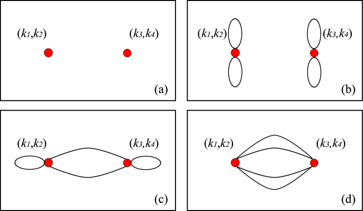
Figure 3: (Color online) Graphs used for the evaluation of the second cumulant (99). (a): empty diagram. (b): graph with no links between the left and right pairs. (c): graph with two links between the left and right pairs. (d): graphs with four links between the left and right pairs.

We start considering graphs with no links between the left and right pairs, see Fig. 3b. The sum of this class of graphs is

$$[0-\textrm{link}]=[1\;2,3\;4]+[1\;2,4\;3]+[2\;1,3\;4]+[2\;1,4\;3]=4\;[1\;2,3\;4].$$ (109)

We have

$$\qquad[1\;2,3\;4] = {\sum_{k}}\Delta(k_{1},k_{2};k_{1},k_{2})\Delta(k_{3},k_{4};k_{3},k_{4})=\sum_{k}g(0,k_{1}\oplus k_{2})\;g(0,k_{3}\oplus k_{4}).$$ (110)

By setting $l_{2}=k_{1}\oplus k_{2}$ and $l_{3}=k_{1}\oplus k_{3}$, we get

$$\quad[1\;2,3\;4]=\sum_{k_{1},k_{4}}\sum_{l_{2},l_{3}}g(0,l_{2})\;g(0,l_{3})=N^{2}\sum_{l_{2},l_{3}}g(0,l_{2})g(0,l_{3})=N^{2}\Big{(}\sum_{k}g(0,k)\Big{)}^{2}.$$ (111)

Therefore, by using (92), we get

$$[0-\textrm{link}]=4\;[1\;2,3\;4]=N^{2}{(N_{A}+N_{\bar{A}})}^{2}.$$ (112)

Let us now consider the graphs with two links between left and right pairs in Fig. 3c. The sum of this class of graphs is

$$[2-\textrm{link}] = [1\;3,2\;4]+[1\;3,4\;2]+[3\;1,2\;4]+[3\;1,4\;2]$$ (113)

$$+ [2\;3,1\;4]+[2\;3,4\;1]+[3\;2,1\;4]+[3\;2,4\;1]$$

$$+ [1\;4,2\;3]+[1\;4,3\;2]+[4\;1,2\;3]+[4\;1,3\;2]$$

$$+ [2\;4,1\;3]+[2\;4,3\;1]+[4\;2,1\;3]+[4\;2,3\;1]$$

$$= 16\;[1\;3,2\;4].$$

One gets

$$\quad[1\;3,2\;4] = \sum_{k}\Delta(k_{1},k_{2};k_{1},k_{3})\Delta(k_{3},k_{4};k_{2},k_{4})$$

$$= \sum_{k}g\Big{(}k_{2}\oplus k_{3},(k_{1}\oplus k_{3})\vee(k_{1}\oplus k_{2})\Big{)}\;g\Big{(}k_{2}\oplus k_{3},(k_{2}\oplus k_{4})\vee(k_{3}\oplus k_{4})\Big{)}.$$

By setting $l_{1}=k_{1}\oplus k_{3}$, $l_{2}=k_{2}\oplus k_{3}$, and $l_{4}=k_{3}\oplus k_{4}$ we get

$$\qquad[1\;3,2\;4] = \sum_{k_{3}}\sum_{l_{1},l_{2},l_{4}}g\Big{(}l_{2},l_{1}\vee(l_{1}\oplus l_{2})\Big{)}\;g\Big{(}l_{2},(l_{2}\oplus l_{4})\vee l_{4}\Big{)}$$ (115)

$$= N\sum_{l_{1},l_{2},l_{4}}g(l_{2},l_{1}\vee l_{2})\;g(l_{2},l_{2}\vee l_{4}),$$

where we have used the (easy to prove) useful relation

$$l_{1}\vee(l_{1}\oplus l_{2})=l_{1}\vee l_{2}.$$ (116)

We get

$$l_{2}\wedge(l_{1}\vee l_{2})=(l_{1}\wedge l_{2})\vee l_{2},$$ (117)

so that the constraint of the function $g$, $l_{2}\wedge(l_{1}\vee l_{2})=0$, implies that $l_{2}=0$. Therefore, by using (92), we obtain

$$[2-\textrm{link}]=16\;[1\;3,2\;4]=16N\Big{(}\sum_{k}g(k,0)\Big{)}^{2}=4N(N_{A}+N_{\bar{A}})^{2}.$$ (118)

The contribution of the graphs with four links between left and right pairs (see Fig. 3d) has the form

$$[4-\textrm{link}]=[3\;4,1\;2]+[4\;3,2\;1]+[4\;3,1\;2]+[3\;4,2\;1]=4[3\;4,1\;2].$$ (119)

We have

$$[3\;4,1\;2] = {\sum_{k}}\Delta(k_{1},k_{2};k_{3},k_{4})\Delta(k_{3},k_{4};k_{1},k_{2})={\sum_{k}}\Delta(k_{1},k_{2};k_{3},k_{4})^{2}$$ (120)

$$= {\sum_{k}}g\bigg{(}(k_{1}\oplus k_{3})\vee(k_{2}\oplus k_{4}),(k_{1}\oplus k_{4})\vee(k_{2}\oplus k_{3})\bigg{)}^{2}.$$

By setting $l_{1}=k_{1}\oplus k_{3}$, $l_{4}=k_{1}\oplus k_{4}$, and $l_{2}=k_{1}\oplus k_{2}\oplus k_{3}\oplus k_{4}$, we get

$$[3\;4,1\;2]=\sum_{k_{3}}\sum_{l_{1},l_{2},l_{4}}g(l_{1}\vee l_{2},l_{4}\vee l_{2})^{2}=N\sum_{l_{1},l_{4}}g(l_{1},l_{4})^{2},$$ (121)

where we used the relation (116) and the constraint $l_{2}=0$ implied by $(l_{1}\vee l_{2})\wedge(l_{4}\vee l_{2})=0$. Therefore, we get

$$[4-\textrm{link}]=4[3\;4,1\;2]=Nf_{2}(N),$$ (122)

where

$$f_{2}(N)=4\sum_{k,l\in{\mathbb{Z}}_{2}^{n}}g(k,l)^{2}.$$ (123)

Notice that if

$$d=|A\cap\bar{B}|=|B\cap\bar{A}|\in[0,n_{A}].$$ (124)

is the distance between bipartitions $(A,\bar{A})$ and $(B,\bar{B})$, defined as the number of qubits belonging to $A$ and not to $B$, then

$$f_{2}(N)=2\left(\!\!\begin{array}[]{c}n\\ n_{A}\end{array}\!\!\right)^{\!\!\!-1}\!\!\!\sum_{0\leq d\leq n_{A}}\!\!\left(\!\!\begin{array}[]{c}n_{A}\\ d\end{array}\!\!\right)\left(\!\!\begin{array}[]{c}n_{\bar{A}}\\ d\end{array}\!\!\right)2^{n/2}\left[4^{n/4-d}+4^{-(n/4-d)}\right].$$ (131)

See B. Summing up, we obtain

$$\qquad\sum_{p\in\mathcal{P}_{4}}[p(1)\;p(2),p(3)\;p(4)] = [0-\textrm{link}]+[2-\textrm{link}]+[4-\textrm{link}]$$ (132)

$$= 4[1\;2,3\;4]+16[1\;3,2\;4]+4[3\;4,1\;2]$$

$$= N(N+4)(N_{A}+N_{\bar{A}})^{2}+Nf_{2}(N).$$

Therefore,

$$\langle H^{2}\rangle_{0}=\frac{f_{2}(N)+(N+4)(N_{A}+N_{\bar{A}})^{2}}{(N+1)(N+2)(N+3)},$$ (133)

and

$$\bar{\sigma}^{2}=\frac{(N+1)f_{2}(N)-2(N_{A}+N_{\bar{A}})^{2}}{(N+1)^{2}(N+2)(N+3)}.$$ (134)

We have checked that the above analytic expression of the second cumulant, with $f_{2}$ given by Eq. (123), agrees very well (within 1% up to $n=8$) with the numerical estimates based on the probability density function (obtained by sampling $5\times 10^{4}$ typical states for each value of $n$).

Finally, one proves that (see B), in the limit $N\to\infty$,

$$f_{2}(N)\sim 3\sqrt{2}N^{\alpha},$$ (135)

with

$$\alpha=\log_{2}3-1\simeq 0.5850.$$ (136)

Therefore, for $N\to\infty$ we have

$$\bar{\sigma}^{2}\sim\frac{f_{2}(N)}{N^{3}}=\frac{3\sqrt{2}}{N^{4-\log_{2}3}}=O(N^{-2.415}).$$ (137)

Incidentally, note that

$$\bar{\sigma}^{2}=\left(\!\!\begin{array}[]{c}n\\ n_{A}\end{array}\!\!\right)^{\!\!-2}\sum_{A,B}\left[\left\langle\pi_{A}\pi_{B}\right\rangle_{0}-\left\langle\pi_{A}\right\rangle_{0}\left\langle\pi_{B}\right\rangle_{0}\right],$$ (138)

so that, if the bipartitions were independent, we would have obtained

$$\bar{\sigma}^{2}_{\mathrm{ind}}=\left(\!\!\begin{array}[]{c}n\\ n_{A}\end{array}\!\!\right)^{\!\!-2}\sum_{A}\left[\left\langle\pi_{A}^{2}\right\rangle_{0}-\left\langle\pi_{A}\right\rangle_{0}^{2}\right]=\left(\!\!\begin{array}[]{c}n\\ n_{A}\end{array}\!\!\right)^{\!\!-1}\sigma^{2}\sim N^{-3}.$$ (139)

Thus, the result in Eq. (137) detects an interference among different bipartitions. We stress that the asymptotic estimate is very accurate even for small values of $n$. In Fig. 4 we plot the difference between the analytic value of second cumulant, obtained using Eq. (134) with $f_{2}$ given by Eq. (123), and its asymptotic limit, obtained by substituting (135) into Eq. (134). We notice an oscillatory behavior: the asymptotic expression systematically overestimates (underestimates) the second cumulant for even (odd) values of $n$. On the other hand, the approximation is very good even for small values of $n$.

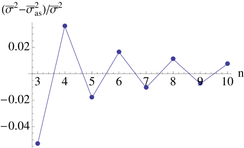
Figure 4: (Color online) Difference between the analytic value of second cumulant, computed according to Eq. (134) with $f_{2}$ given by (123), and its asymptotic limit, obtained by substituting (135) into Eq. (134). The approximation is valid within a few percent even for $n=3$.

5.3 Third cumulant

The third cumulant is defined as

$$\kappa_{0}^{(3)}[H]=\left\langle\left(H-\langle H\rangle_{0}\right)^{3}\right\rangle_{0}=\langle H^{3}\rangle_{0}-3\langle H^{2}\rangle_{0}\langle H\rangle_{0}+2\langle H\rangle_{0}^{3}.$$ (140)

In analogy with the evaluation of the second cumulant we have

$$\langle H^{3}\rangle_{0}=\langle|z_{1}|^{2}|z_{2}|^{2}|z_{3}|^{2}|z_{4}|^{2}|z_{5}|^{2}|z_{6}|^{2}\rangle_{0}\sum_{p\in\mathcal{P}_{6}}[p(1)\;p(2),p(3)\;p(4),p(5)\;p(6)],$$

with

$$[p(1)\;p(2),p(3)\;p(4),p(5)\;p(6)] = {\sum_{k\in\mathbb{Z}_{2}^{6n}}}\Delta(k_{1},k_{2};k_{p(1)},k_{p(2)})$$

$$\times \Delta(k_{3},k_{4};k_{p(3)},k_{p(4)})\Delta(k_{5},k_{6};k_{p(5)},k_{p(6)})$$

and $\mathcal{P}_{6}$ the permutation group of $\{1,2,3,4,5,6\}$. From Eq. (62) we easily obtain

$$\langle|z_{1}|^{2}|z_{2}|^{2}|z_{3}|^{2}|z_{4}|^{2}|z_{5}|^{2}|z_{6}|^{2}\rangle_{0}=\frac{1}{N(N+1)(N+2)(N+3)(N+4)(N+5)}.$$

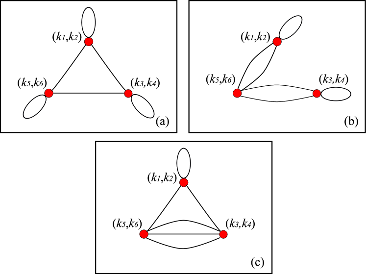
Figure 5: (Color online) Non-oriented connected graphs used for the evaluation of the third cumulant. (a): three ears. (b): two ears. (c): one ear.

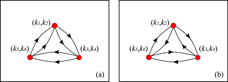
Figure 6: (Color online) Oriented connected graphs used for the evaluation of the third cumulant. (a): same internal and external orientations of the edges (nonvanishing “current”). (b): opposite internal and external orientations of the edges (vanishing “current”).

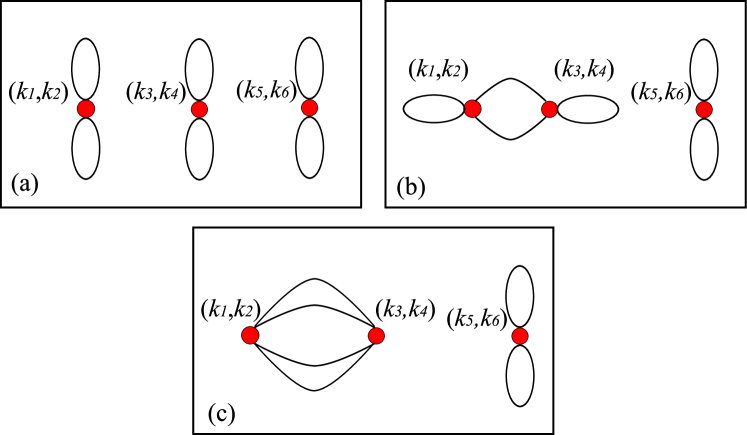
Figure 7: (Color online) Disconnected graphs used for the evaluation of the third cumulant. (a): six loops. (b): four loops. (c): two loops.

We start by considering connected graphs with three ears. A representative of this equivalence class is depicted in Fig. 5a. We have

$$\quad[1\;6,3\;2,5\;4] = \sum_{k}\Delta(k_{1},k_{2};k_{1},k_{6})\Delta(k_{3},k_{4};k_{3},k_{2})\Delta(k_{5},k_{6};k_{5},k_{4})$$ (144)

$$= \sum_{k}g\Big{(}k_{2}\oplus k_{6},(k_{1}\oplus k_{6})\vee(k_{1}\oplus k_{2})\Big{)}\;g\Big{(}k_{2}\oplus k_{4},(k_{2}\oplus k_{3})\vee(k_{3}\oplus k_{4})\Big{)}$$

$$\times g\Big{(}k_{4}\oplus k_{6},(k_{4}\oplus k_{5})\vee(k_{5}\oplus k_{6})\Big{)}$$

$$= \sum_{k_{1},k_{2},k_{3},k_{5}}g(0,k_{1}\oplus k_{2})\;g(0,k_{2}\oplus k_{3})\;g(0,k_{2}\oplus k_{5})$$

$$= N\Big{(}\sum_{k}g(0,k)\Big{)}^{3}=N\frac{(N_{A}+N_{\bar{A}})^{3}}{8},$$

where the constraint in the definition of the function $g$ has implied $k_{2}=k_{4}=k_{6}$ and we used Eq. (92). The degeneracy of this class of graphs is $128$.

We now consider the class of connected graphs with two ears represented in Fig. 5b. We obtain

$$\quad[1\;3,2\;5,4\;6] = \sum_{k}\Delta(k_{1},k_{2};k_{1},k_{3})\Delta(k_{3},k_{4};k_{2},k_{5})\Delta(k_{5},k_{6};k_{4},k_{6})$$ (145)

$$= \sum_{k_{1},k_{2},k_{4},k_{6}}g(k_{1}\oplus k_{2},0)\;g(k_{2}\oplus k_{4},0)\;g(k_{4}\oplus k_{6},0)$$

$$= N\Big{(}\sum_{k}g(k,0)\Big{)}^{3}=N\frac{(N_{A}+N_{\bar{A}})^{3}}{8},$$

where we have imposed $k_{2}=k_{3}$ and $k_{4}=k_{5}$. The degeneracy of the class is $192$.

The final class of non-oriented connected graphs is represented in Fig. 5c. Its explicit calculation yields

$$\quad[1\;6,2\;5,3\;4] = \sum_{k}\Delta(k_{1},k_{2};k_{1},k_{6})\Delta(k_{3},k_{4};k_{2},k_{5})\Delta(k_{5},k_{6};k_{3},k_{4})$$ (146)

$$= \sum_{k}g\Big{(}k_{2}\oplus k_{6},(k_{1}\oplus k_{6})\vee(k_{1}\oplus k_{2})\Big{)}$$

$$\times g\Big{(}(k_{2}\oplus k_{3})\vee(k_{4}\oplus k_{5}),(k_{3}\oplus k_{5})\vee(k_{2}\oplus k_{4})\Big{)}$$

$$\times g\Big{(}(k_{3}\oplus k_{5})\vee(k_{4}\oplus k_{6}),(k_{4}\oplus k_{5})\vee(k_{3}\oplus k_{6})\Big{)}$$

$$= \sum_{k_{1},...,k_{5}}g(0,k_{1}\oplus k_{2})g\Big{(}(k_{2}\oplus k_{3})\vee(k_{4}\oplus k_{5}),(k_{3}\oplus k_{5})\vee(k_{2}\oplus k_{4})\Big{)}^{2}$$

$$= \sum_{k_{1},...,k_{5}}g(0,k_{1}\oplus k_{2})g(k_{2}\oplus k_{3},k_{2}\oplus k_{4})^{2}$$

$$= N\sum_{k}g(0,k)\sum_{l_{1},l_{2}}g(l_{1},l_{2})^{2}=N\frac{N_{A}+N_{\bar{A}}}{2}\sum_{l_{1},l_{2}}g(l_{1},l_{2})^{2}$$

$$= N\frac{N_{A}+N_{\bar{A}}}{8}f_{2}(N),$$

where we have used the constraint $k_{2}=k_{6}$ and the function $f_{2}(N)$ defined in Eq. (123). The degeneracy of this graph is $192$.

In order to take into account the contribution of connected graphs with no ears, it is necessary to consider two different classes of oriented graphs whose representatives are shown in Figs. 6a and 6b, respectively. For the first class (Fig. 6a, nonvanishing “current”) we have

$$\quad[5\;6,1\;2,3\;4] = \sum_{k}\Delta(k_{1},k_{2};k_{5},k_{6})\Delta(k_{3},k_{4};k_{1},k_{2})\Delta(k_{5},k_{6};k_{3},k_{4})$$ (147)

$$= \sum_{k}g\Big{(}(k_{1}\oplus k_{5})\vee(k_{2}\oplus k_{6}),(k_{1}\oplus k_{6})\vee(k_{2}\oplus k_{5})\Big{)}$$

$$\times g\Big{(}(k_{1}\oplus k_{3})\vee(k_{2}\oplus k_{4}),(k_{2}\oplus k_{3})\vee(k_{1}\oplus k_{4})\Big{)}$$

$$\times g\Big{(}(k_{3}\oplus k_{5})\vee(k_{4}\oplus k_{6}),(k_{4}\oplus k_{5})\vee(k_{3}\oplus k_{6})\Big{)}$$

$$= \sum_{k_{1},k_{2},k_{3},k_{5}}g(k_{1}\oplus k_{5},k_{2}\oplus k_{5})\;g(k_{1}\oplus k_{3},k_{2}\oplus k_{3})$$

$$\times g(k_{3}\oplus k_{5},k_{1}\oplus k_{2}\oplus k_{3}\oplus k_{5})$$

$$= N\sum_{k_{1},k_{2},k_{3}}g(k_{1},k_{2})\;g(k_{1}\oplus k_{3},k_{2}\oplus k_{3})\;g(k_{3},k_{1}\oplus k_{2}\oplus k_{3})$$

$$= N\sum_{k_{1},k_{2},k_{3}}g(k_{1},k_{2}\oplus k_{3})\;g(k_{2},k_{1}\oplus k_{3})\;g(k_{3},k_{1}\oplus k_{2})$$

$$= N\,f_{3}^{(1)}(N)$$

where we have used the constraints $k_{4}=k_{1}\oplus k_{2}\oplus k_{3}$ and $k_{6}=k_{1}\oplus k_{2}\oplus k_{5}$ and defined

$$f_{3}^{(1)}(N)=\sum_{k_{1},k_{2},k_{3}}g(k_{1},k_{2}\oplus k_{3})\;g(k_{2},k_{1}\oplus k_{3})\;g(k_{3},k_{1}\oplus k_{2}).$$ (148)

The degeneracy of this graph is $16$. An analogous calculation can be carried out for the second class of oriented graphs (Fig. 6b, vanishing “current”). We obtain

$$\quad[3\;6,5\;2,1\;4] = \sum_{k}\Delta(k_{1},k_{2};k_{3},k_{6})\Delta(k_{3},k_{4};k_{5},k_{2})\Delta(k_{5},k_{6};k_{1},k_{4})$$ (149)

$$= N\sum_{k_{1},k_{2},k_{3}}g(k_{1},k_{2})\;g(k_{3},k_{2})\;g(k_{1}\oplus k_{3},k_{2})=N\,f_{3}^{(0)}(N)$$

with

$$f_{3}^{(0)}(N)=\sum_{k_{1},k_{2},k_{3}}g(k_{1},k_{2})\;g(k_{3},k_{2})\;g(k_{1}\oplus k_{3},k_{2}).$$ (150)

In this case, the degeneracy is $64$.

The contribution of disconnected graphs (Fig. 7) can be computed by considering the results obtained for the first and second cumulant. For the class of graphs represented in Fig. 7a we have

$$\quad[1\;2,3\;4,5\;6] = N^{3}\frac{(N_{A}+N_{\bar{A}})^{3}}{8},$$ (151)

with degeneracy $8$. In the case of the graph in Fig. 7b the result is

$$\quad[1\;3,2\;4,5\;6] = N\frac{(N_{A}+N_{\bar{A}})^{2}}{4}N\frac{(N_{A}+N_{\bar{A}})}{2}=N^{2}\frac{(N_{A}+N_{\bar{A}})^{3}}{8},$$ (152)

with degeneracy $96$. Finally from the disconnected graphs with two loops (Fig. 7c) we obtain

$$\quad[3\;4,1\;2,5\;6] = N^{2}\frac{(N_{A}+N_{\bar{A}})}{8}f_{2}(N),$$ (153)

with degeneracy $24$. In conclusion, we find

$$\langle H^{3}\rangle_{0} = \frac{1}{(N+1)(N+2)(N+3)(N+4)(N+5)}$$ (154)

$$\times\Big{(}16f_{3}^{(1)}(N)+64f_{3}^{(0)}(N)+3(N+8)(N_{A}+N_{\bar{A}})f_{2}(N)$$

$$\qquad+(N_{A}+N_{\bar{A}})^{3}(N^{2}+12N+40)\Big{)}$$

and, therefore,

$$\qquad\kappa_{0}^{(3)}[H] = \frac{1}{(N+1)^{3}(N+2)(N+3)(N+4)(N+5)}$$

$$\times\Big{(}16(N+1)^{2}f_{3}^{(1)}(N)+64(N+1)^{2}f_{3}^{(0)}(N)$$

$$\qquad-36(N+1)(N_{A}+N_{\bar{A}})f_{2}(N)-8(N_{A}+N_{\bar{A}})^{3}(N-5)\Big{)}.$$ (155)

We have checked that the above analytic expression of the third cumulant, with $f_{2}$, $f_{3}^{(0)}$ and $f_{3}^{(1)}$ given by (123), (150) and (148), respectively, agrees very well (less than 1% for $n=1\div 7$ and a few % for $n=8$) with the numerical estimates based on the probability density function (obtained by sampling $5\times 10^{4}$ typical states for each value of $n$).

Finally, in the limit $N\to\infty$, one can prove that (see C)

$$f_{3}^{(0)}(N)\sim c\,N^{5-\gamma},$$ (156)

with $c\simeq 1.05385$ and $\gamma\simeq 4.1583$ given by (286) and (287), and that (see D)

$$f_{3}^{(1)}(N)\sim N^{\alpha},$$ (157)

with $\alpha\simeq 0.5850$ given by (136). Therefore, by recalling the asymptotic expression for $f_{2}(N)$ (135), we find that the graph in Fig. 6b dominates over that in Fig. 6a and

$$\kappa_{0}^{(3)}[H] \sim 64\,c\,N^{-\gamma}\simeq 67.443\,N^{-4.1583}.$$ (158)

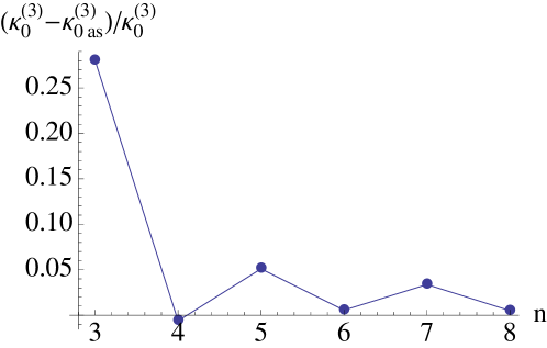
Figure 8: (Color online) Difference between the analytic value of third cumulant, computed according to Eq. (5.3) with $f_{2}$, $f_{3}^{(0)}$ and $f_{3}^{(1)}$ given by (123), (150), (150), and their asymptotic limits, obtained by substituting (135), (156), (157) into Eq. (5.3). The approximation is valid within a few percent for $n\geq 4$.

In Fig. 8 we plot the difference between the analytic value of third cumulant and its asymptotic limit, obtained by substituting (135), (156), (157) into Eq. (5.3). We again observe an oscillating behaviour. The approximation is good for $n\geq 4$.

5.4 Gaussian approximation

We can now summarize the results obtained for the first three cumulants and try to get a broader picture. Equations (97), (134) and (5.3) are all exact. Their asymptotic expansions for large $N$, are given in Eqs. (98), (137) and (158). By plugging these results into Eqs. (56) and (57) we obtain the asymptotic expressions of the average energy

$$\langle H\rangle_{\beta} \sim \frac{2}{\sqrt{N}}-\beta\frac{3\sqrt{2}}{N^{3-\alpha}}+\frac{\beta^{2}}{2}\frac{64c}{N^{\gamma}}$$ (159)

$$\simeq \frac{2}{N^{0.5}}-\beta\frac{4.243}{N^{2.415}}+\frac{\beta^{2}}{2}\frac{67.443}{N^{4.1583}}$$

and the free energy

$$F(\beta) \sim \frac{\ln Z(0)}{\beta}-\frac{2}{\sqrt{N}}+\frac{\beta}{2}\frac{3\sqrt{2}}{N^{3-\alpha}}-\frac{\beta^{2}}{6}\frac{64c}{N^{\gamma}}$$ (160)

$$\simeq \frac{\ln Z(0)}{\beta}-\frac{2}{N^{0.5}}+\frac{\beta}{2}\frac{4.243}{N^{2.415}}-\frac{\beta^{2}}{6}\frac{67.443}{N^{4.1583}}$$

where

$$c\simeq 1.054,\quad\alpha=\log_{2}3-1\simeq 0.5850,\quad\gamma=4.1583.$$ (161)

See Eqs. (286) and (287).

If $N$ is large enough and the first two cumulants at $\beta=0$ suffice, the energy distribution (42) can be taken to be Gaussian

$$P_{0}(E)\sim\frac{1}{\sqrt{2\pi\bar{\sigma}^{2}}}\exp\left(-\frac{\left(E-\mu\right)^{2}}{2\bar{\sigma}^{2}}\right),$$ (162)

where $\mu$ and $\bar{\sigma}$ are given in (98) and (137), respectively. The energy distribution at arbitrary temperature is then [see Eq. (52)]

$$P_{\beta}(E)\sim\frac{1}{\sqrt{2\pi\bar{\sigma}^{2}}}\exp\left(-\frac{\left(E-\mu+\beta\bar{\sigma}^{2}\right)^{2}}{2\bar{\sigma}^{2}}\right).$$ (163)

This is valid for relatively small $\beta$:

$$\mu-\beta\bar{\sigma}^{2}-\bar{\sigma}\gtrsim 0\quad\Leftrightarrow\quad\beta\lesssim\mu/\bar{\sigma}^{2}\sim N^{7/2-\log_{2}3}.$$ (164)

Up to this value the probability density rigidly shifts with $\beta$, as is apparent in Fig. 2, which was obtained by numerically solving Eq. (43).

5.5 A few comments

The behavior of the cumulants derived in this section is very peculiar. The second and third cumulant follow a nontrivial power dependence, with trascendental exponents [see Eqs. (159)]). Interestingly, close scrutiny of the calculation in Sec. 5.3 shows also that $3-\alpha$, the exponent that governs the $N$-dependence of $\bar{\sigma}^{2}$, is found in a class of (nondominant) graphs that appear in the evaluation of the third cumulant: the exponent $5-\alpha$ stems from the graph in Fig. 6a (the dominant exponent $\gamma$ stemming from the graph in Fig. 6b). This might suggest a possible recursion of the exponent $\alpha$ at all orders in the cumulant expansion. At this stage, we are unable to say if at higher orders the dominant graph for $\kappa_{0}^{(3)}$ in Fig. 6b cancels, yielding a series in $N^{q(\alpha)}$ with $q$ a function of $\alpha$.

It would be important to go beyond the Gaussian approximation in order to evaluate the behaviour of the left tail of the probability density function, close to $\pi_{\mathrm{ME}}=E\simeq E_{0}$. See Figs. 1 and 2. This would give us some precious information about the features of MMES and the very structure of entanglement frustration [24]. In particular, it would be interesting to understand the role played by the interference among the bipartitions, in connection with the appearance of frustration in MMESs. See for instance the asymptotic behavior of the second cumulant in Eqs. (137)-(139) and the short discussion that follows. Additional investigation is necessary in order to elucidate these intriguing issues.

6 Concluding remarks and outlook

We have built a statistical mechanical approach to multipartite entanglement, by introducing a partition function in order to tackle a complex optimization problem, whose solutions are the maximally multipartite entangled states, that appear as minimal energy configurations.

The scheme adopted here is general. In classical statistical mechanics, temperature is used to fix the energy to a given value in the thermodynamic limit. Analogously, the fictitious temperature introduced here localizes the measure on a set of states whose entanglement (energy) is fixed, and can be larger or smaller than the entanglement associated to typical states.

Remarkably, a strategy like the one adopted in this article, when applied to the simpler case of bipartite entanglement (at a fixed bipartition) [47] brings to light an involved landscape of phase transitions for the purity. Clearly, the multipartite version of the problem is much more involved, as the picture that emerges is complex and unearths a remarkable interplay between multipartite entanglement and frustration. It would therefore be of great interest to understand whether the phase transition that occurs in the bipartite situation, when there is no average over the bipartitions, survives and has a counterpart in the multipartite scenario. This possibility will be explored in the future.

One important property that we have not investigated here and that is often used to characterize multipartite entanglement is the so-called monogamy of entanglement [15, 48], that essentially states that entanglement cannot be freely shared among the parties. Interestingly, although monogamy is a typical property of multipartite entanglement, it is expressed in terms of a bound on a sum of bipartite entanglement measures. This is reminiscent of the approach taken in this paper. The curious fact that bipartite sharing of entanglement is bounded might have interesting consequences in the present context. It would be worth understanding whether monogamy of entanglement generates frustration.

Finally, we think that the characterization of multipartite entanglement proposed here can be important for the analysis of the entanglement features of many-body systems, such as spin systems and systems close to criticality.

Appendix A

We derive here the expression (24) of the coupling function. See [46]. We start from the definition (23), that can be rewritten as

$$\Delta(k,k^{\prime};l,l^{\prime})=\frac{1}{2}\left(\!\!\begin{array}[]{c}n\\ n_{A}\end{array}\!\!\right)^{\!\!-1}\left(\tilde{\Delta}(k,k^{\prime};l,l^{\prime};[n/2])+\tilde{\Delta}(k^{\prime},k;l,l^{\prime};[n/2])\right),$$ (165)

where

$$\tilde{\Delta}(k,k^{\prime};l,l^{\prime};n_{A})=\sum_{|A|=n_{A}}\delta_{k_{A},l^{\prime}_{A}}\delta_{k^{\prime}_{A},l_{A}}\delta_{k_{\bar{A}},l_{\bar{A}}}\delta_{k^{\prime}_{\bar{A}},l^{\prime}_{\bar{A}}}.$$ (166)

Let us fix a quadruple of binary strings $(k,k^{\prime},l,l^{\prime})$ and a dimension $n_{A}$. See figure 9. A bipartition $(A,\bar{A})$, with $|A|=n_{A}$ yields a nonvanishing contribution to the sum (166) when

$$\delta_{k_{A},l^{\prime}_{A}}\delta_{k^{\prime}_{A},l_{A}}\delta_{k_{\bar{A}},l_{\bar{A}}}\delta_{k^{\prime}_{\bar{A}},l^{\prime}_{\bar{A}}}=1,$$ (167)

that is when

$$k_{A}=l^{\prime}_{A},\quad k^{\prime}_{A}=l_{A},\quad k_{\bar{A}}=l_{\bar{A}},\quad k^{\prime}_{\bar{A}}=l^{\prime}_{\bar{A}},$$ (168)

where we recall that $k_{A}=l_{A}$ means that the substrings of $k$ and $l$ are equal, namely $k_{i}=l_{i}$ for all $i\in A$. By noting that two bits $k_{i}$ and $l_{i}$ are equal when $k_{i}\oplus l_{i}=0$, the above condition can be rephrased as

$$k_{A}\oplus l^{\prime}_{A}=0,\quad k^{\prime}_{A}\oplus l_{A}=0,\quad k_{\bar{A}}\oplus l_{\bar{A}}=0,\quad k^{\prime}_{\bar{A}}\oplus l^{\prime}_{\bar{A}}=0,$$ (169)

that is

$$(k_{A}\oplus l^{\prime}_{A})\vee(k^{\prime}_{A}\oplus l_{A})=0,\quad(k_{\bar{A}}\oplus l_{\bar{A}})\vee(k^{\prime}_{\bar{A}}\oplus l^{\prime}_{\bar{A}})=0.$$ (170)

Summarizing, a bipartition $(A,\bar{A})$ yields a nonvanishing contribution to (23) if and only if the following substrings are zero

$$a_{\bar{A}}=0\quad\mathrm{and}\quad b_{A}=0,$$ (171)

where

$$a=(k\oplus l)\vee(k^{\prime}\oplus l^{\prime})\quad\mathrm{and}\quad b=(k\oplus l^{\prime})\vee(k^{\prime}\oplus l).$$ (172)

Note that equation (171) implies that

$$a\wedge b=0,$$ (173)

since $(a\wedge b)_{A}=a_{A}\wedge 0=0$ and $(a\wedge b)_{\bar{A}}=0\wedge b_{\bar{A}}=0$. On the other hand, the substrings $a_{A}$ and $b_{\bar{A}}$ are totally free, whence

$$|a|=|a_{A}|\leq|A|=n_{A},\qquad|b|=|b_{\bar{A}}|\leq|\bar{A}|=n_{\bar{A}}.\qquad$$ (174)

It is easy to see that (173) and (174) are also sufficient conditions for the existence of a partition $(A,\bar{A})$ that satisfies (171).

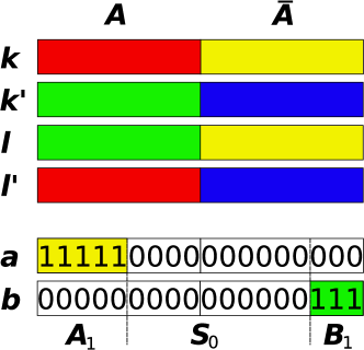
Figure 9: (Color online) Graphic representation of the combination of binary strings contributing to sum (166).

In conclusion, $\tilde{\Delta}(k,k^{\prime};l,l^{\prime};n_{A})\neq 0$ when

$$a\wedge b=0,\quad\mbox{ with }\quad|a|\leq n_{A},\,|b|\leq n_{\bar{A}}.$$ (175)

Therefore,

$$\qquad\tilde{\Delta}(k,k^{\prime};l,l^{\prime};n_{A})=\delta_{a\wedge b,\,0}\;\chi_{[0,n_{A}]}(|a|)\;\chi_{[0,n_{\bar{A}}]}(|b|)\;\#(k,k^{\prime},l,l^{\prime}),$$ (176)

where $\chi_{G}$ is the characteristic function of set $G$ and $\#(k,k^{\prime},l,l^{\prime})$ the number of terms in the sum in (165) that contribute to the function $\tilde{\Delta}$.

Note that, since by (175) the strings $a$ and $b$ cannot be both $1$ at the same position, the set $S$ is partitioned into three disjoint subsets (see figure 9)

$$S=S_{0}\cup A_{1}\cup B_{1},$$ (177)

where

$$S_{0} = \{i\in S\,|\,a_{i}=0,\;b_{i}=0\},$$

$$A_{1} = \{i\in S\,|\,a_{i}=1,\;b_{i}=0\},$$

$$B_{1} = \{i\in S\,|\,a_{i}=0,\;b_{i}=1\}.$$ (178)

Obviously, $|A_{1}|=|a|\leq n_{A}$ and $|B_{1}|=|b|\leq n_{\bar{A}}$.

The number of terms $\#(k,k^{\prime},l,l^{\prime})$ is given by the number of bipartitions $(A,\bar{A})$ with $|A|=n_{A}$ such that

$$A_{1}\subset A\quad\mathrm{and}\quad B_{1}\subset\bar{A}.$$ (179)

Since $A\cap\bar{A}=\emptyset$, parties $A$ and $\bar{A}$ contend for $S_{0}$, namely

$$A=A_{1}\cup(S_{0}\cap A)\quad\mbox{and}\quad\bar{A}=B_{1}\cup(S_{0}\cap\bar{A}).$$ (180)

Thus, the number of bipartition is the number of ways of picking $|A\backslash A_{1}|$ unordered outcomes from $|S_{0}|$ possibilities. Since $|A\backslash A_{1}|=|A|-|A_{1}|=n_{A}-|a|$ and $|S_{0}|=|S|-|A_{1}|-|B_{1}|=n-|a|-|b|$, one gets

$$\#(k,k^{\prime},l,l^{\prime})=\left(\begin{array}[]{c}n-|a|-|b|\\ {n_{A}}-|a|\end{array}\right).$$ (183)

Substituting Eq. (183) into Eq. (176) and by defining the binomial coefficient to be identically zero when its arguments are negative, we notice that the characteristic functions in (176) yield always one, and obtain Eq. (24).

Appendix B

We derive here the asymptotic (for large $N$) behavior of the function $f_{2}(N)$ defined in Eq. (135). Let us define the distance between bipartitions $(A,\bar{A})$ and $(B,\bar{B})$ as the number of qubits belonging to $A$ and not to $B$

$$d=|A\cap\bar{B}|=|B\cap\bar{A}|\in[0,n_{A}].$$ (184)

The number of pairs of bipartitions at a distance $d$ is

$$n_{d}=\left(\begin{array}[]{c}n\\ n_{A}\end{array}\right)\left(\begin{array}[]{c}n_{A}\\ d\end{array}\right)\left(\begin{array}[]{c}n_{\bar{A}}\\ d\end{array}\right).$$ (191)

Therefore the sum over the bipartitions can be rewritten as a sum over $d$

$$\sum_{|A|,|B|=n_{A}}[\cdots]=\left(\begin{array}[]{c}n\\ n_{A}\end{array}\right)\sum_{d=0}^{n_{A}}\left(\begin{array}[]{c}n_{A}\\ d\end{array}\right)\left(\begin{array}[]{c}n_{\bar{A}}\\ d\end{array}\right)[\cdots].$$ (198)

Let us consider for instance

$$\quad\sum_{k,l\in{\mathbb{Z}}_{2}^{n}}{g(k,l)}^{2} = \frac{1}{N}\sum_{k\in{\mathbb{Z}}_{2}^{4n}}{\Delta(k_{1},k_{2};k_{3},k_{4})}^{2}$$

$$= \frac{1}{N}\left(\!\!\begin{array}[]{c}n\\ n_{A}\end{array}\!\!\right)^{\!\!\!-2}\sum_{k}\sum_{|A|,|B|=n_{A}}\frac{1}{4}\Big{(}\delta(k;A)\delta(k;B)+\delta(k;A)\delta(k;\bar{B})$$

$$\qquad\qquad\qquad\qquad\qquad\quad+\delta(k;\bar{A})\delta(k;B)+\delta(k;\bar{A})\delta(k;\bar{B})\Big{)}$$

$$= \frac{1}{N}\left(\!\!\begin{array}[]{c}n\\ n_{A}\end{array}\!\!\right)^{\!\!\!-2}\sum_{k}\sum_{|A|,|B|=n_{A}}\frac{1}{2}\Big{(}\delta(k;A)\delta(k;B)+\delta(k;A)\delta(k;\bar{B})\Big{)},$$ (204)

where

$$\delta(k,k^{\prime},l,l^{\prime};A)=\delta_{k_{A},l^{\prime}_{A}}\delta_{k^{\prime}_{A},l_{A}}\delta_{k_{\bar{A}},l_{\bar{A}}}\delta_{k^{\prime}_{\bar{A}},l^{\prime}_{\bar{A}}}$$ (205)

Let us start by showing that

$$h(A,B)=\sum_{k}\delta(k;A)\delta(k;B)=\sum_{k,k^{\prime},l,l^{\prime}}\delta_{k_{A},l^{\prime}_{A}}\delta_{k^{\prime}_{A},l_{A}}\delta_{k_{B},l^{\prime}_{B}}\delta_{k^{\prime}_{B},l_{B}}\delta_{k_{\bar{A}},l_{\bar{A}}}\delta_{k^{\prime}_{\bar{A}},l^{\prime}_{\bar{A}}}\delta_{k_{\bar{B}},l_{\bar{B}}}\delta_{k^{\prime}_{\bar{B}},l^{\prime}_{\bar{B}}}$$ (206)

depends only on $d=|A\cap\bar{B}|$. When $A=B$, i.e. $d=0$,

$$\qquad h(A,A)=\sum_{k}\delta(k;A)^{2}=\sum_{k}\delta(k;A)=\sum_{k,k^{\prime},l,l^{\prime}}\delta_{k_{A},l^{\prime}_{A}}\delta_{k^{\prime}_{A},l_{A}}\delta_{k_{\bar{A}},l_{\bar{A}}}\delta_{k^{\prime}_{\bar{A}},l^{\prime}_{\bar{A}}}=N^{2},$$ (207)

while, when $d\neq 0$, we get

$$h(A,B)=\left(\frac{N}{2^{d}}\right)^{2}=4^{-d}N^{2}.$$ (208)

Therefore, we get

$$\sum_{k}\sum_{|A|,|B|=n_{A}}\delta(k;A)\delta(k;B)=\sum_{|A|,|B|=n_{A}}h(A,B)$$

$$=\sum_{0\leq d\leq n_{A}}n_{d}\;4^{-d}N^{2}=\left(\!\!\begin{array}[]{c}n\\ n_{A}\end{array}\!\!\right)\!\sum_{0\leq d\leq n_{A}}\!\!4^{-d}\left(\!\!\begin{array}[]{c}n_{A}\\ d\end{array}\!\!\right)\left(\!\!\begin{array}[]{c}n_{\bar{A}}\\ d\end{array}\!\!\right).$$ (215)

Analogously we find

$$\sum_{k}\sum_{|A|,|B|=n_{A}}\delta(k;A)\delta(k;\bar{B})=\left(\!\!\begin{array}[]{c}n\\ n_{A}\end{array}\!\!\right)\!\sum_{0\leq d\leq n_{A}}\!\!4^{d}\left(\!\!\begin{array}[]{c}n_{A}\\ d\end{array}\!\!\right)\left(\!\!\begin{array}[]{c}n_{\bar{A}}\\ d\end{array}\!\!\right).$$ (222)

Putting together Eqs. (215)-(222) we get

$$f_{2}(N) = 4\sum_{k,l}g(k,l)^{2}$$ (229)

$$= 2\left(\!\!\begin{array}[]{c}n\\ n_{A}\end{array}\!\!\right)^{\!\!\!-1}\!\!\!\sum_{0\leq d\leq n_{A}}\!\!\left(\!\!\begin{array}[]{c}n_{A}\\ d\end{array}\!\!\right)\left(\!\!\begin{array}[]{c}n_{\bar{A}}\\ d\end{array}\!\!\right)(4^{n/2-d}+4^{d})=$$

$$= 2\left(\!\!\begin{array}[]{c}n\\ n_{A}\end{array}\!\!\right)^{\!\!\!-1}\!\!\!\sum_{0\leq d\leq n_{A}}\!\!\left(\!\!\begin{array}[]{c}n_{A}\\ d\end{array}\!\!\right)\left(\!\!\begin{array}[]{c}n_{\bar{A}}\\ d\end{array}\!\!\right)2^{n/2}\left[4^{n/4-d}+4^{-(n/4-d)}\right].$$ (236)

We notice that the terms in the summation strongly depend on the ratio $2d/n$. In the limit $n\rightarrow+\infty$ only the terms with $d=n/6$ and $d=n/3$ give a significant contribution to the summation (see Fig. 10).

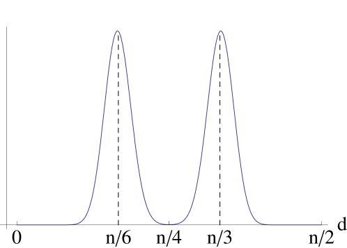
Figure 10: (Color online) $d$-dependence of the terms $\left(\!\!\begin{array}[]{c}n_{A}\\ d\end{array}\!\!\right)\left(\!\!\begin{array}[]{c}n_{\bar{A}}\\ d\end{array}\!\!\right)2^{n/2}\left[4^{n/4-d}+4^{-(n/4-d)}\right]$ in the sum (236).

Let us consider the case of even $n$ (in the thermodynamic limit the result for an odd number of qubits is the same)

$$n_{A}=n_{\bar{A}}=n/2.$$ (237)

By Stirling’s approximation $n!\sim(n/e)^{n}\sqrt{2\pi n}$ (for $n$ large) and by defining the new variable

$$x=\frac{2d}{n},$$ (238)

after a straightforward calculation we obtain

$$f_{2}(N) \sim 2\sqrt{\frac{\pi n}{2}}2^{-n}\sum_{d}\frac{1}{\pi nx\left(1-x\right)}\exp{\left\{nS(x)\right\}}2^{n/2}\left[4^{\frac{n}{2}(\frac{1}{2}-x)}+4^{-\frac{n}{2}(\frac{1}{2}-x)}\right]$$ (239)

$$\sim \sqrt{2\pi n}\int_{0}^{1}\mathrm{d}x\frac{1}{2\pi x(1-x)}$$

$$\times \left[\exp{\left\{n\left[S(x)-x\ln 2\right]\right\}}+2^{-n}\exp{\left\{n\left[S(x)+x\ln 2\right]\right\}}\right],$$

where

$$S(x)=-x\ln x-(1-x)\ln(1-x)$$ (240)

is the Shannon entropy. Using the saddle point approximation in the integrand we get

$$f_{2}(N) \sim \sqrt{2\pi n}\int_{0}^{1}\mathrm{d}x\frac{9}{4\pi}$$ (241)

$$\times \left[\exp{\left\{n\left[S\left(\frac{1}{3}\right)-\frac{1}{3}\ln 2+\frac{1}{2}S^{\prime\prime}\left(\frac{1}{3}\right){(x-\frac{1}{3})}^{2}\right]\right\}}+\right.$$

$$+ \left.2^{-n}\exp{\left\{n\left[S\left(\frac{2}{3}\right)+\frac{2}{3}\ln 2+\frac{1}{2}S^{\prime\prime}\left(\frac{2}{3}\right){(x-\frac{2}{3})}^{2}\right]\right\}}\right]$$

$$= \sqrt{2\pi n}\int_{0}^{1}\mathrm{d}x\frac{9}{4\pi}\exp\left\{n\ln\frac{3}{2}\right\}$$

$$\times \left[\exp\left\{-n\frac{9}{4}{\left(x-\frac{1}{3}\right)}^{2}\right\}+\exp\left\{-n\frac{9}{4}{\left(x-\frac{2}{3}\right)}^{2}\right\}\right]$$

$$\sim \frac{9}{\sqrt{2\pi}}{\left(\frac{3}{2}\right)}^{n}\int_{-\infty}^{+\infty}\mathrm{d}x\exp\left\{-\frac{9}{4}x^{2}\right\}=3\sqrt{2}N^{\alpha},$$

where

$$\alpha=\log_{2}3-1\simeq 0.584963.$$ (242)

This is the asymptotic expression (135) used in Eq. (137).

Appendix C

We evaluate here the asymptotic behavior of the function $f_{3}^{(0)}(N)$ defined in (150). By using the definition (25), (150) can be written

$$f_{3}^{(0)}(N) = \sum_{k_{1},k_{2},k_{3}}g(k_{1},k_{2})\;g(k_{3},k_{2})\;g(k_{1}\oplus k_{3},k_{2})$$

$$= \sum_{k_{1},k_{2},k_{3}}\delta_{k_{1}\wedge k_{2},0}\delta_{k_{2}\wedge k_{3},0}\delta_{k_{2}\wedge(k_{1}\oplus k_{3}),0}$$

$$\times \hat{g}(|k_{1}|,|k_{2}|)\;\hat{g}(|k_{3}|,|k_{2}|)\;\hat{g}(|k_{1}\oplus k_{3}|,|k_{2}|)$$

$$= \sum_{s_{0},s_{1},s_{2},s_{3}}f(s_{0},s_{1},s_{2},s_{3})\hat{g}(s_{1},s_{2})\;\hat{g}(s_{3},s_{2})\;\hat{g}(s_{1}+s_{3}-2s_{0},s_{2}),$$

where

$$f(s_{0},s_{1},s_{2},s_{3})=\sum_{k_{1},k_{2},k_{3}}\delta_{k_{1}\wedge k_{2},0}\delta_{k_{2}\wedge k_{3},0}\delta_{s_{1},|k_{1}|}\delta_{s_{2},|k_{2}|}\delta_{s_{3},|k_{3}|}\delta_{s_{0},|k_{1}\wedge k_{3}|}$$ (244)

and we have used

$$k_{1}\wedge k_{2}=0,\quad k_{2}\wedge k_{3}=0\quad\Rightarrow\quad k_{2}\wedge(k_{1}\oplus k_{3})=0,$$ (245)

$$|k_{1}\oplus k_{3}|=|k_{1}|+|k_{3}|-2|k_{1}\wedge k_{3}|.$$ (246)

It is straightforward to count the number of terms in (244) and obtain

$$f(s_{0},s_{1},s_{2},s_{3}) = \left(\!\!\begin{array}[]{c}n\\ s_{2}\end{array}\!\!\right)\left(\!\!\begin{array}[]{c}n-s_{2}\\ s_{1}\end{array}\!\!\right)\left(\!\!\begin{array}[]{c}s_{1}\\ s_{0}\end{array}\!\!\right)\left(\!\!\begin{array}[]{c}n-s_{2}-s_{1}\\ s_{3}-s_{0}\end{array}\!\!\right)$$ (255)

$$= \frac{n!}{s_{2}!s_{0}!(s_{1}-s_{0})!(s_{3}-s_{0})!(n-s_{2}-s_{1}-s_{3}+s_{0})!}.$$ (256)

By substituting $s_{1}\to s_{1}+s_{0}$ and $s_{3}\to s_{3}+s_{0}$ in Eq. (C) we obtain

$$f_{3}^{(0)}(N) = \sum_{s_{0},s_{1},s_{2},s_{3}}\frac{n!}{s_{0}!s_{1}!s_{2}!s_{3}!(n-s_{1}-s_{2}-s_{3}-s_{0})!}$$ (259)

$$\times \hat{g}(s_{1}+s_{0},s_{2})\;\hat{g}(s_{3}+s_{0},s_{2})\;\hat{g}(s_{1}+s_{3},s_{2})$$

$$= \sum_{s}\left(\!\!\begin{array}[]{c}n\\ s_{0},s_{1},s_{2},s_{3}\end{array}\!\!\right)\hat{g}(s_{1}+s_{0},s_{2})\;\hat{g}(s_{3}+s_{0},s_{2})\;\hat{g}(s_{1}+s_{3},s_{2}),$$

where

$$\left(\!\!\begin{array}[]{c}n\\ i_{1},i_{2},...,i_{k}\end{array}\!\!\right)=\frac{n!}{\Pi_{j=1}^{k}(i_{j}!)(n-\sum_{j=1}^{k}i_{j})!}$$ (263)

denotes the multinomial coefficient. A relabeling of the dummy variables yields

$$\qquad f_{3}^{(0)}(N)=\sum_{s}\left(\!\!\begin{array}[]{c}n\\ s_{0},s_{1},s_{2},s_{3}\end{array}\!\!\right)\hat{g}(s_{1}+s_{2},s_{0})\;\hat{g}(s_{2}+s_{3},s_{0})\;\hat{g}(s_{3}+s_{1},s_{0}).$$ (264)

From the definition (32) one easily get

$$\hat{g}(s,t)=\frac{1}{2}\left(\!\!\begin{array}[]{c}n\\ s,t\end{array}\!\!\right)^{\!\!-1}\left[\left(\!\!\begin{array}[]{c}n_{A}\\ s\end{array}\!\!\right)\left(\!\!\begin{array}[]{c}n_{\bar{A}}\\ t\end{array}\!\!\right)+\left(\!\!\begin{array}[]{c}n_{A}\\ t\end{array}\!\!\right)\left(\!\!\begin{array}[]{c}n_{\bar{A}}\\ s\end{array}\!\!\right)\right].$$ (265)

Therefore, for $n_{A}=n_{\bar{A}}=n/2$ we finally obtain

$$\quad f_{3}^{(0)}(N)=\sum_{s}\left(\!\!\begin{array}[]{c}n\\ s_{0},s_{1},s_{2},s_{3}\end{array}\!\!\right)\left(\!\!\begin{array}[]{c}n/2\\ s_{0}\end{array}\!\!\right)^{\!\!3}\prod_{1\leq i\leq 3}\left(\!\!\begin{array}[]{c}n\\ s_{0},s_{i}+s_{i+1}\end{array}\!\!\right)^{\!\!-1}\left(\!\!\begin{array}[]{c}n/2\\ s_{i}+s_{i+1}\end{array}\!\!\right).$$ (266)

Now, by using the Stirling approximation and scaling the variables

$$\sigma_{0}=\frac{s_{0}}{n},\;\sigma_{1}=\frac{s_{1}}{n},\;\sigma_{2}=\frac{s_{2}}{n},\;\sigma_{3}=\frac{s_{3}}{n}$$ (267)

we obtain, after some algebra, the asymptotic form

$$f_{3}^{(0)}(N)\sim\frac{1}{(2\pi n)^{2}}\sum_{s}A(\sigma_{0},\sigma_{1},\sigma_{2},\sigma_{3})\,\exp\{nS(\sigma_{0},\sigma_{1},\sigma_{2},\sigma_{3})\}.$$ (268)

In Eq. (268) we have set (with the implicit convention that the indices are cyclical)

$$\quad A=\sqrt{\frac{\prod_{i=1}^{3}(1-\sigma_{0}-\sigma_{i}-\sigma_{i+1})}{\sigma_{0}(1-2\sigma_{0})^{3}(1-\sigma_{0}-\sigma_{1}-\sigma_{2}-\sigma_{3})\prod_{i=1}^{3}\sigma_{i}(1-2\sigma_{i}-2\sigma_{i+1})}}$$ (269)

and

$$S(\sigma_{0},\sigma_{1},\sigma_{2},\sigma_{3}) = S_{4}(\sigma_{0},\sigma_{1},\sigma_{2},\sigma_{3})-S_{2}(\sigma_{0},\sigma_{1}+\sigma_{2})-S_{2}(\sigma_{0},\sigma_{2}+\sigma_{3})$$ (270)

$$- S_{2}(\sigma_{0},\sigma_{3}+\sigma_{1})+\frac{3}{2}S_{1}(2\sigma_{0})+\frac{1}{2}S_{1}(2\sigma_{1}+2\sigma_{2})$$

$$+ \frac{1}{2}S_{1}(2\sigma_{2}+2\sigma_{3})+\frac{1}{2}S_{1}(2\sigma_{3}+2\sigma_{1}),$$

with

$$S_{n}(x_{1},\dots,x_{n})=-\sum_{i=1}^{n}x_{i}\log x_{i}-\Big{(}1-\sum_{i=1}^{n}x_{i}\Big{)}\log\!\Big{(}1-\sum_{i=1}^{n}x_{i}\Big{)}.$$ (271)

By noting that

$$S_{n}(x_{1},\dots,x_{n})=\sum_{i=1}^{n}x_{i}\frac{\partial S_{n}}{\partial x_{i}}-\log\!\Big{(}1-\sum_{i=1}^{n}x_{i}\Big{)},$$ (272)

one easily gets

$$S=\sigma_{0}\frac{\partial S}{\partial\sigma_{0}}+\sum_{i=1}^{3}\sigma_{i}\frac{\partial S}{\partial\sigma_{i}}+S_{0},$$ (273)

with

$$\qquad S_{0}=\frac{1}{2}\log\frac{\prod_{i=1}^{3}(1-\sigma_{0}-\sigma_{i}-\sigma_{i+1})^{2}}{(1-\sigma_{0}-\sigma_{1}-\sigma_{2}-\sigma_{3})^{2}(1-2\sigma_{0})^{3}\prod_{i=1}^{3}(1-2\sigma_{i}-2\sigma_{i+1})}.$$ (274)

In the limit $n\to\infty$ the main contribution comes from the saddle point $(\sigma_{0}^{*},\sigma_{1}^{*},\sigma_{2}^{*},\sigma_{3}^{*})$, solution to the system

$$\frac{\partial S}{\partial\sigma_{i}}=0,\mbox{with}\;\;i=0,1,2,3,$$ (275)

that reads

$$(1-\sigma_{0}-\sigma_{1}-\sigma_{2}-\sigma_{3})\left(1-2\sigma_{0}\right)^{3}=8\sigma_{0}\prod_{i=1}^{3}(1-\sigma_{0}-\sigma_{i}-\sigma_{i+1}),$$ (276)

$$(1-\sigma_{0}-\sigma_{1}-\sigma_{2}-\sigma_{3})\left(1-2\sigma_{i}-2\sigma_{i+1}\right)\left(1-2\sigma_{i}-2\sigma_{i+2}\right)$$

$$\quad=4\sigma_{i}(1-\sigma_{0}-\sigma_{i}-\sigma_{i+1})(1-\sigma_{0}-\sigma_{i}-\sigma_{i+2}),$$ (277)

with $i=1,2,3$. In the limit $n\to\infty$ we get

$$\quad f_{3}^{(0)}(N) \sim \left(\frac{n}{2\pi}\right)^{2}A^{*}\mathrm{e}^{nS_{0}^{*}}\int_{\mathbb{R}^{4}}\exp\left(\frac{n}{2}\sum_{i,j=0}^{3}\frac{\partial^{2}S^{*}}{\partial\sigma_{i}\partial\sigma_{j}}(\sigma_{i}-\sigma_{i}^{*})(\sigma_{j}-\sigma_{j}^{*})\right)\mathrm{d}\sigma_{0}\mathrm{d}\sigma_{1}\mathrm{d}\sigma_{2}\mathrm{d}\sigma_{3}$$

$$= A^{*}\det\left(\frac{\partial^{2}S^{*}}{\partial\sigma_{i}\partial\sigma_{j}}\right)^{-1/2}\exp\left(nS_{0}^{*}\right)$$ (278)

where the starred functions $A^{*}$, $S^{*}$, and $\partial^{2}S^{*}/\partial\sigma_{i}\partial\sigma_{j}$ are evaluated at the saddle point $(\sigma_{0}^{*},\sigma_{1}^{*},\sigma_{2}^{*},\sigma_{3}^{*})$.

The symmetry of the equations suggests to look at a symmetric solution of (277) with

$$\sigma_{i}=\sigma\quad\mbox{with}\;\;i=1,2,3,$$ (279)

which yields

$$(1-\sigma_{0}-3\sigma)(1-2\sigma_{0})^{3}=8\sigma_{0}(1-\sigma_{0}-2\sigma)^{3},$$

$$(1-\sigma_{0}-3\sigma)(1-4\sigma)^{2}=4\sigma(1-\sigma_{0}-2\sigma)^{2}.$$ (280)

We get

$$\quad A^{*}=\sqrt{\frac{(1-\sigma_{0}^{*}-2\sigma^{*})^{3}}{\sigma_{0}^{*}\sigma^{*3}(1-2\sigma_{0}^{*})^{3}(1-4\sigma^{*})^{3}(1-\sigma_{0}^{*}-3\sigma^{*})}}=\sqrt{\frac{1}{8\sigma_{0}^{*2}\sigma^{*3}(1-4\sigma^{*})^{3}}},$$ (281)

$$\quad S_{0}^{*}=\frac{1}{2}\log\frac{(1-\sigma_{0}^{*}-2\sigma^{*})^{6}}{(1-\sigma_{0}^{*}-3\sigma^{*})^{2}(1-2\sigma_{0}^{*})^{3}(1-4\sigma^{*})^{3}}=\frac{1}{2}\log\frac{(1-2\sigma_{0}^{*})^{3}}{64\sigma_{0}^{*2}(1-4\sigma^{*})^{3}},$$ (282)

and

$$\quad\det\left(\frac{\partial^{2}S^{*}}{\partial\sigma_{i}\partial\sigma_{j}}\right) = \frac{(1-\sigma_{0}^{*}-5\sigma^{*}+2\sigma^{*}(4\sigma^{*}+\sigma_{0}^{*}))^{2}}{\sigma_{0}^{*}\sigma^{*3}(1-2\sigma_{0}^{*})(1-4\sigma^{*})^{3}(1-\sigma_{0}^{*}-3\sigma^{*})(1-\sigma_{0}^{*}-2\sigma^{*})^{3}}$$ (283)

$$\times(1-2\sigma^{*}-\sigma_{0}^{*2}-4\sigma^{*2}+4\sigma^{*}\sigma_{0}^{*}(8\sigma^{*}+2\sigma_{0}^{*}-3))$$

The solution of the system that gives the largest contribution is

$$\sigma_{0}^{*} = \frac{13}{36}-\frac{13}{36\sqrt[3]{197-18\sqrt{113}}}-\frac{1}{36}\sqrt[3]{197-18\sqrt{113}}\simeq 0.108955,$$

$$\sigma^{*} = -\frac{5043923}{144\left(197-18\sqrt{113}\right)^{7/3}}+\frac{158161\sqrt{113}}{48\left(197-18\sqrt{113}\right)^{7/3}}$$ (284)

$$+\frac{980473}{72\left(197-18\sqrt{113}\right)^{2}}-\frac{2561\sqrt{113}}{2\left(197-18\sqrt{113}\right)^{2}}$$

$$-\frac{18119}{144\left(197-18\sqrt{113}\right)^{5/3}}+\frac{563\sqrt{113}}{48\left(197-18\sqrt{113}\right)^{5/3}}$$

$$\simeq 0.104767.$$

Plugging these results into Eq. (278) we get

$$f_{3}^{(0)}(N)\sim c\;N^{5-\gamma}$$ (285)

where

$$c = A^{*}\det\left(\frac{\partial^{2}S^{*}}{\partial\sigma_{i}\partial\sigma_{j}}\right)^{-1/2}$$ (286)

$$= \frac{(1-\sigma_{0}^{*}-2\sigma^{*})^{3}}{1-2\sigma_{0}^{*}}$$

$$\times\frac{1}{(1-\sigma_{0}^{*}-5\sigma^{*}+2\sigma^{*}(4\sigma^{*}+\sigma_{0}^{*}))\sqrt{1-2\sigma^{*}-\sigma_{0}^{*2}-4\sigma^{*2}+4\sigma^{*}\sigma_{0}^{*}(8\sigma^{*}+2\sigma_{0}^{*}-3)}}$$

$$\simeq 1.05385,$$

and

$$\gamma=5-S_{0}^{*}\log_{2}\mathrm{e}=5-\frac{1}{2}\log_{2}\left[\frac{(1-2\sigma_{0}^{*})^{3}}{64\sigma_{0}^{*2}(1-4\sigma^{*})^{3}}\right]\simeq 4.1583.$$ (287)

Appendix D

We evaluate here the asymptotic behavior of the function $f_{3}^{(1)}(N)$ defined in (148). By using the definition (25) we have

$$f_{3}^{(1)}(N) = \sum_{k_{1},k_{2},k_{3}}g(k_{1},k_{2}\oplus k_{3})\;g(k_{2},k_{1}\oplus k_{3})\;g(k_{3},k_{1}\oplus k_{2})$$ (288)

$$= \sum_{k_{1},k_{2},k_{3}}\delta_{k_{1}\wedge(k_{2}\oplus k_{3}),0}\delta_{k_{2}\wedge(k_{1}\oplus k_{3}),0}\delta_{k_{3}\wedge(k_{1}\oplus k_{2}),0}$$

$$\times\hat{g}(|k_{1}|,|k_{2}\oplus k_{3}|)\;\hat{g}(|k_{2}|,|k_{1}\oplus k_{3}|)\;\hat{g}(|k_{3}|,|k_{1}\oplus k_{3}|)$$

$$= \sum_{s_{0},s_{1},s_{2},s_{3}}h(s_{0},s_{1},s_{2},s_{3})\hat{g}(s_{1},s_{2}+s_{3}-2s_{0})\;\hat{g}(s_{2},s_{1}+s_{2}-2s_{0})$$

$$\times\hat{g}(s_{3},s_{1}+s_{2}-2s_{0}),$$

where

$$h(s_{0},s_{1},s_{2},s_{3})=\sum_{k_{1},k_{2},k_{3}}\delta_{s_{1},|k_{1}|}\delta_{s_{2},|k_{2}|}\delta_{s_{3},|k_{3}|}\delta_{s_{0},|k_{1}\wedge k_{2}|}\delta_{s_{0},|k_{1}\wedge k_{3}|}\delta_{s_{0},|k_{2}\wedge k_{3}|}$$

and we have used

$$k_{1}\wedge(k_{2}\oplus k_{3})=0,\quad k_{2}\wedge(k_{1}\oplus k_{3})=0,\quad k_{3}\wedge(k_{1}\oplus k_{2})=0$$

$$\Rightarrow k_{1}\wedge k_{2}=k_{1}\wedge k_{3}=k_{2}\wedge k_{3},$$

$$|k_{i}\oplus k_{j}|=|k_{i}|+|k_{j}|-2|k_{i}\wedge k_{j}|\quad\forall\;i,j=1,2,3.$$ (290)

We find

$$\quad h(s_{0},s_{1},s_{2},s_{3}) = \frac{n!}{s_{0}!(s_{1}-s_{0})!(s_{2}-s_{0})!(s_{3}-s_{0})!(n-s_{2}-s_{1}-s_{3}+2s_{0})!}.$$ (291)

Using the substitution $s_{1}\to s_{1}+s_{0}$, $s_{2}\to s_{2}+s_{0}$ and $s_{3}\to s_{3}+s_{0}$ in Eq. (288) we obtain

$$\quad f_{3}^{(1)}(N)=\sum_{s}\left(\!\!\begin{array}[]{c}n\\ s_{0},s_{1},s_{2},s_{3}\end{array}\!\!\right)\hat{g}(s_{1}+s_{0},s_{2}+s_{3})\;\hat{g}(s_{2}+s_{0},s_{1}+s_{3})\;\hat{g}(s_{3}+s_{0},s_{1}+s_{2}),$$ (294)

in terms of the multinomial coefficient (263). Using (265 ) for $n_{A}=n_{\bar{A}}=n/2$ we finally obtain

$$\quad f_{3}^{(1)}(N)=\sum_{s}\left(\!\!\begin{array}[]{c}n\\ s_{0},s_{1},s_{2},s_{3}\end{array}\!\!\right)\prod_{1\leq i\leq 3}\left(\!\!\begin{array}[]{c}n\\ s_{0}+s_{i},s_{i+1}+s_{i+2}\end{array}\!\!\right)^{\!\!-1}\left(\!\!\begin{array}[]{c}n/2\\ s_{0}+s_{i}\end{array}\!\!\right)\left(\!\!\begin{array}[]{c}n/2\\ s_{i}+s_{i+1}\end{array}\!\!\right).$$ (304)

Using the Stirling approximation and Eq. (267) we get

$$f_{3}^{(1)}(N)\sim\frac{1}{(2\pi n)^{2}}\sum_{s}A(\sigma_{0},\sigma_{1},\sigma_{2},\sigma_{3})\,\exp\{nS(\sigma_{0},\sigma_{1},\sigma_{2},\sigma_{3})\},$$ (306)

where

$$\qquad A(\sigma_{0},\sigma_{1},\sigma_{2},\sigma_{3})=\frac{(1-\sigma_{0}-\sigma_{1}-\sigma_{2}-\sigma_{3})}{\sqrt{\sigma_{0}\sigma_{1}\sigma_{2}\sigma_{3}\prod_{1\leq i\leq 3}(1-2\sigma_{0}-2\sigma_{i})(1-2\sigma_{i+1}-2\sigma_{i+2})}}$$ (307)

and

$$\qquad S(\sigma_{0},\sigma_{1},\sigma_{2},\sigma_{3}) = S_{4}(\sigma_{0},\sigma_{1},\sigma_{2},\sigma_{3})-S_{2}(\sigma_{0}+\sigma_{1},\sigma_{2}+\sigma_{3})$$ (308)

$$-S_{2}(\sigma_{0}+\sigma_{2},\sigma_{3}+\sigma_{1})-S_{2}(\sigma_{0}+\sigma_{3},\sigma_{1}+\sigma_{2})$$

$$+\frac{1}{2}S_{1}(2\sigma_{0}+2\sigma_{1})+\frac{1}{2}S_{1}(2\sigma_{0}+2\sigma_{2})+\frac{1}{2}S_{1}(2\sigma_{0}+2\sigma_{3})$$

$$+\frac{1}{2}S_{1}(2\sigma_{1}+2\sigma_{2})+\frac{1}{2}S_{1}(2\sigma_{2}+2\sigma_{3})+\frac{1}{2}S_{1}(2\sigma_{3}+2\sigma_{1}),$$

with the entropies defined in Eq. (271). By (272) one gets (273) with

$$S_{0}=\frac{1}{2}\log\frac{(1-\sigma_{0}-\sigma_{1}-\sigma_{2}-\sigma_{3})^{4}}{\prod_{1\leq i\leq 3}(1-2\sigma_{0}-2\sigma_{i})(1-2\sigma_{i+1}-2\sigma_{i+2})}.$$ (309)

In the limit $n\rightarrow+\infty$ we can use the saddle point approximation. The saddle point is solution to the set of equations

$$\frac{\partial S}{\partial\sigma_{i}}=0,\quad\mbox{with}\;\;i=0,1,2,3,$$ (310)

that reads

$$\quad(1-2\sigma_{i}-2\sigma_{i+1})(1-2\sigma_{i}-2\sigma_{i+2})(1-2\sigma_{i}-2\sigma_{i+3})=8\sigma_{i}(1-\sigma_{0}-\sigma_{1}-\sigma_{2}-\sigma_{3})^{2}.$$

The symmetric solution, $\sigma_{i}=\sigma$ for all $i$, corresponds to the largest contribution and is given by

$$\sigma*=\frac{1}{12}.$$ (312)

As in (278), in the limit $n\to\infty$ we get

$$f_{3}^{(1)}(N)\sim A^{*}\det\left(\frac{\partial^{2}S^{*}}{\partial\sigma_{i}\partial\sigma_{j}}\right)^{-1/2}\exp\left(nS_{0}^{*}\right),$$ (313)

with

$$\qquad A^{*}=\frac{1}{\sigma^{*2}(1-4\sigma^{*})^{2}}=324,\qquad\det\left(\frac{\partial^{2}S^{*}}{\partial\sigma_{i}\partial\sigma_{j}}\right)=\frac{1}{\sigma^{*4}(1-4\sigma^{*})^{4}}=324^{2},$$ (314)

and

$$S_{0}^{*}=\log\frac{1}{(1-4\sigma^{*})}=\log\frac{3}{2}.$$ (315)

We finally get

$$f_{3}^{(1)}(N)\sim\mathrm{e}^{n\log(3/2)}=N^{\alpha},\qquad\mbox{for}\quad N\to\infty,$$ (316)

with

$$\alpha={\log_{2}3-1}\simeq 0.584963.$$ (317)

References

References

• [1] Schrödinger E 1935 Proc. Cambridge Phil. Soc. 31 555.
• [2] Schrödinger E 1936 Proc. Cambridge Phil. Soc. 32 446.
• [3] Einstein A, Podolsky B and Rosen N 1935 Phys. Rev. 47 777.
• [4] Wootters W K 2001 Quantum Inf. and Comp. 1 27.
• [5] Amico L, Fazio R, Osterloh A and Vedral V 2008 Rev. Mod. Phys. 80 517.
• [6] Horodecki R, Horodecki P, Horodecki M and Horodecki K 2009 Rev. Mod. Phys. 81, 865.
• [7] Bennett C H and Wiesner S J 1992 Phys. Rev. Lett. 69 2881.
• [8] Bennett C H, Brassard G, Crepeau C, Jozsa R, Peres A and Wootters W K 1993 Phys. Rev. Lett. 70 1895.
• [9] Bennett C H and Brassard G 1984 “Quantum Cryptography: Public Key Distribution and Coin Tossing”, Proceedings of IEEE International Conference on Computers Systems and Signal Processing (Bangalore India) pp 175-179.
• [10] Ekert A 1991 Phys. Rev. Lett. 67 661.
• [11] Deutsch D, Ekert A, Rozsa P, Macchiavello C, Popescu S and Sanpera A 1996 Phys. Rev. Lett. 77 2818.
• [12] Fuchs C A, Gisin N, Griffiths R B, Niu C-S and Peres A, Phys. Rev. A 1997 56 1163.
• [13] Wootters W K 1998 Phys. Rev. Lett. 80 2245.
• [14] Bennett C H, DiVincenzo D P, Smolin J A and Wootters W K 1996 Phys. Rev. A 54 3824.
• [15] Coffman V, Kundu J and Wootters W K 2000 Phys. Rev. A 61 052306.
• [16] Wong A and Christensen N 2001 Phys. Rev. A 63 044301.
• [17] Bruss D 2002 J. Math. Phys. 43 4237.
• [18] Meyer D A and Wallach N R 2002 J. Math. Phys. 43, 4273.
• [19] M. Jakob and J. Bergou 2007 Phys. Rev. A 76 052107.
• [20] Facchi P, Florio G, Marzolino U, Parisi G and Pascazio S 2009 J. Phys. A: Math. Theor. 42 055304.
• [21] Facchi P, Florio G and Pascazio S 2006 Phys. Rev. A 74 042331; 2007 Int. J. Quantum Inf. 5 97.
• [22] Mezard M, Parisi G and Virasoro M A, 1987 Spin Glass Theory and Beyond (World Scientific, Singapore).
• [23] Man’ko V I, Marmo G, Sudarshan E C G and Zaccaria F 2002 J. Phys. A: Math. Gen. 35 7137.
• [24] Facchi P, Florio G, Marzolino U, Parisi G and Pascazio S 2010 New J. Phys. 12 025015.
• [25] Horodecki M, Horodecki P, and Horodecki R 1998 Phys. Rev. Lett. 80 5239.
• [26] Bennett C H, DiVincenzo D P, Mor T, Shor P W, Smolin J A, and Terhal B M 1999 Phys. Rev. Lett. 82, 5385.
• [27] Scott A J 2004 Phys. Rev. A 69 052330.
• [28] Parthasarathy K R 2004 Proc. Indian Acad. Sciences 114 365.
• [29] Facchi P, Florio G, Parisi G and Pascazio S 2008 Phys. Rev. A 77 060304(R).
• [30] Greenberger D M, Horne M and Zeilinger A 1990 Am. J. Phys. 58 1131.
• [31] Higuchi A and Sudbery A 2000 Phys. Lett. A 273 213.
• [32] Brown I D K, Stepney S, Sudbery A, and Braunstein 2005 J. Phys. A: Math. Gen. 38 1119.
• [33] Brierley S and Higuchi A 2007 J. Phys. A: Math. Gen. 40 8455.
• [34] Facchi P, Florio G, Lupo C, Mancini S and Pascazio S 2009 Phys. Rev. A 80 062311.
• [35] Lubkin E 1978 J. Math. Phys. 19 1028.
• [36] Lloyd S and Pagels H 1988 Ann. Phys. NY 188 186.
• [37] Page D N 1993 Phys. Rev. Lett. 71 1291.
• [38] Życzkowski K and Sommers H J 2001 J. Phys. A 34 7111.
• [39] Scott A J and Caves C M 2003 J. Phys. A: Math. Gen. 36 9553.
• [40] Giraud O 2007 J. Phys. A: Math. Theor. 40 2793.
• [41] Mejia-Monasterio C, Benenti G, Carlo G G, and Casati G 2005 Phys. Rev. A 71 062324.
• [42] Rossini D and Benenti G 2008 Phys. Rev. Lett. 100 060501.
• [43] M. M. Sinolecka, K. Zyczkowski, M. Kus, Acta Physica Polonica B 33, 2081 (2002).
• [44] Kirkpatrick S, Gelatt C D Jr. and Vecchi M P 1983 Science 220 671.
• [45] Marinari E and Parisi G 1992 Europhys. Lett. 19 451.
• [46] Facchi P 2009 Rend. Lincei Mat. Appl. 20 25-67.
• [47] Facchi P, Marzolino U, Parisi G, Pascazio S and Scardicchio A 2008 Phys. Rev. Lett. 101 050502.
• [48] Kim J S, Das A and Sanders B C 2009 Phys. Rev. A 79 012329.