The Hubble constant inferred from 18 time-delay lenses

Abstract

We present a simultaneous analysis of 18 galaxy lenses with time delay measurements. For each lens we derive mass maps using pixelated simultaneous modeling with shared Hubble constant. We estimate the Hubble constant to be $66_{-4}^{+6}$ $\rm{km}$ $\rm{s}^{-1}\rm{Mpc}^{-1}$ (for a flat Universe with $\Omega_{m}=0.3$, $\Omega_{\Lambda}=0.7$). We have also selected a subsample of five relatively isolated early type galaxies and by simultaneous modeling with an additional constraint on isothermality of their mass profiles we get $H_{0}=76_{-3}^{+3}$ $\rm{km}$ $\rm{s}^{-1}\rm{Mpc}^{-1}$.

1 Introduction

The Hubble constant is one of the most important parameters in cosmology. It determines the age of universe, the physical distances to objects, constrains the dark energy equation-of-state and furthermore, it is used as a prior in many cosmological analysis. Hence, it is essential for cosmology to know the precise value of $H_{0}$ (Riess et al., 2009). The newest measurements give a quite well defined $H_{0}$ with estimated errors at the 5-10% level but unfortunately $H_{0}$ differs among different cosmological methods and there is only marginal consistency between their $1\sigma$ errors (see Table 1).

Moreover, those methods are based on different physical principles and more importantly they measure different consequences of $H_{0}$. Both SNe and Cepheids measure luminosity distance but at different scales (distant and local Universe respectively). Cepheids can provide a luminosity distance via the period-luminosity relation but only in the local Universe, on the other hand, the significantly brighter SNe with their characteristic peak luminosity can measure cosmological distances but need to be calibrated with Cepheids. The SZ effect, which is based on high energy electrons in a galaxy cluster distorting the CMB through inverse Compton scattering, is proportional to the gas density of the galaxy cluster and that combined with the cluster’s X-ray flux gives an estimate of the angular diameter distance. Finally, the angular power spectrum of the CMB gives information about many cosmological parameters which have correlated effects on the power spectrum, especially strong degeneracies are between $H_{0}$ and $\Omega_{m}$ and $\Omega_{b}$. Furthermore, there are significant differences in the obtained results even within one method (eg. SNe Branch et al. (1996); Sandage et al. (2006); Riess et al. (2009), see Table 1).

Additionally, any astrophysical approach suffers from systematic uncertainties, e.g., supernovae are not standard but standardized candles with possible redshift evolution, CMB have various parameter degeneracies and interference with foregrounds, and the SZ method is assuming spherical symmetry on often significantly non-spherical clusters of galaxies. It is therefore important to explore complementary methods for measuring $H_{0}$. Gravitationally lensed quasars QSOs offer such an attractive alternative.

Table 1: $H_{0}$ comparison

Method	$H_{0}$	Author
CMB (3 years)	$73.2^{+3.1}_{-3.2}$	Spergel et al. (2007)
CMB (5 years)	$71.9^{+2.6}_{-2.7}$	Komatsu et al. (2009)
Ia SNa	$74.2\pm 3.6$	Riess et al. (2009)
Ia SNa	$62.3\pm 1.3$	Sandage et al. (2006)
SZ	$65^{+8}_{-7}$	Jones et al. (2005)
Cepheids	$72\pm 8$	Freedman et al. (2001)

As shown by Refsdal (1964) the Hubble constant can be measured based on the time delay $\Delta t$ between multiply lensed images of QSOs, because $H_{0}\propto 1/\Delta t$, provided that the mass distribution of the lens is known. Time delays measure $\frac{D_{OL}D_{OS}}{D_{LS}}$, where $D_{\rm OL}$, $D_{\rm OS}$, $D_{\rm LS}$ are the angular diameter distances between observer and lens, observer and source, and lens and source, respectively. Gravitational lensing has its degeneracies but it is based on well understood physics and unlike distance ladder methods there are no calibration issues (Branch et al., 1996; Sandage et al., 2006).

Gravitational lensing has, up to now, not been seen as reliable as other leading cosmological methods. Determination of the Hubble constant using lensing is problematic, because the mass distribution of a lens strongly influences the result of $H_{0}$ and unfortunately we never have a complete knowledge of that, hence a choice of a lens model is needed.

Recently, however, time-delay lenses have successfully been used for $H_{0}$ estimation. In particular, Oguri (2007) used a Monte Carlo method to combine lenses and derived $H_{0}=70\pm 6$ $\rm{km}$ $\rm{s}^{-1}\rm{Mpc}^{-1}$. Saha et al. (2006) obtained $H_{0}=72^{+8}_{-11}$ $\rm{km}$ $\rm{s}^{-1}\rm{Mpc}^{-1}$ using a combination of 10 lenses, Coles (2008) got $H_{0}=71^{+6}_{-8}$ $\rm{km}$ $\rm{s}^{-1}\rm{Mpc}^{-1}$ using a combination of 11 lenses, and Suyu et al. (2009) found $H_{0}=69.7^{+4.9}_{-5.0}$ $\rm{km}$ $\rm{s}^{-1}\rm{Mpc}^{-1}$ by detailed analysis of one gravitational lens, B1608+656.

This paper extends the work of Saha et al. (2006) and Coles (2008), where results on $H_{0}$ were presented using combined modeling of 10 and 11 lenses, respectively. We have used those systems with refined properties of lenses as a part of our sample and have added new systems that have been discovered and monitored during the past 4 years. We therefore now posses an almost doubled sample of systems with measured time delay, which demonstrates that, gravitational lensing is valuable method for $H_{0}$ estimation.

2 Pixelated modeling

Two different approaches for modeling lenses are commonly used. The first one, the non-parametric (pixelated) method, generates a large number of models which perfectly fit the data, each of them giving a different result which can then be averaged. For the second method, model fitting, one assumes parametrized models of the mass distribution of the lens.

Pixelated modeling has the advantage of allowing the lens shape and profile to vary freely. It does not presume any parameters and can provide models that would not be possible to reproduce with parametric modeling. Using this approach to a combined analysis of a large sample of lenses is a powerful solution to the modeling problem in gravitational lensing.

In this paper we use the non-analytical method created by Saha & Williams (2004) - PixeLens. PixeLens generates an ensemble of lens models that fit the input data. Each model consists of a set of discrete mass points, the position of the source and optionally, if the time delays are known, $H_{0}$. The time delay $\Delta\tau$ is the combined effect of the difference in length of the optical path between two images and the gravitational time dilation of two light rays passing through different parts of the lens potential well,

$$\Delta\tau=\frac{1+z_{\rm L}}{c}\frac{D_{\rm OS}D_{\rm OL}}{D_{\rm LS}}\left(\frac{1}{2}(\vec{\theta}-\vec{\beta})^{2}-\Psi(\vec{\theta})\right).$$ (1)

Here $\vec{\theta}$ and $\vec{\beta}$ are the positions of the images and the source respectively, $z_{\rm L}$ is the lens redshift, and $\Psi$ is the effective gravitational potential of the lens.

The arrival time at position $\vec{\theta}$ is defined in PixeLens, as a modeled surface,

$$\tau(\vec{\theta})=\frac{1}{2}|\vec{\theta}|^{2}-\vec{\theta}\cdot\vec{\beta}-\int\ln|\vec{\theta}-\vec{\theta}^{\prime}|\kappa(\vec{\theta}^{\prime})d^{2}\vec{\theta}^{\prime},$$ (2)

where $\kappa$ is surface mass density.

The errors of the positions of observed images and redshifts of source and lens are of the order of a few percent, thus can be ignored. The main source of errors in the data comes from time delays between images.

We have used PixeLens to generate a set of 100 models for a sample of lensing systems (see §3). PixeLens produces an ensemble of models with varying $H_{0}$, each consisting of sets of mass pixels, which exactly reproduce the input data. Moreover, it also models several lenses simultaneously enforcing shared $H_{0}$ for all lenses. The images positions, the source and lens redshifts, and the time delay are assumed to be accurate enough for their errors to be ignored (Saha et al., 2006). PixeLens also imposes secondary constraints on mass maps: non-negative density; smoothness, where the density of a pixel must be no more than twice the average density of its neighbors; the mass profile is required to have $180^{\circ}$ rotation symmetry (except if it appears very asymmetric); the shear is allowed within $45^{\circ}$ of the chosen direction; circularly averaged mass profile should nowhere be shallower nor steeper than $r^{-\alpha_{min}}$ and $r^{-\alpha_{max}}$ respectively, where $\alpha_{min}$ and $\alpha_{max}$ is defined in PixeLens as the minimum and maximum steepness, those values can be chosen by the user however, the default PixeLens constraint is minimal steepness $\alpha_{min}=0.5$; and finally, additional lenses as point masses can be constrained. PixeLens does not use flux ratios as constraints because of the possible influence of reddening by dust (Elíasdóttir et al., 2006), microlensing (Paraficz et al., 2006) or small-scale structure in the lens potential (Dalal & Kochanek, 2002).

3 Data set

To date, there are 19 gravitational lens systems with published time delays. Table 2 summarizes the information about these 19 systems. We have made an attempt to use all the conclusions previously drawn about their shape, external shear, profile, etc. We have used the newest/best measurement of positions and redshifts of images and lens. Apart from the main lensing galaxies we have also included all the galaxies that might contribute to the lensing. We added them whenever they are visible in the field. These systems are RX J0911+055, HE 1104-181, SBS 1520+530, B1600+434 and B1608+656. All the mass maps of the doubly imaged quasars are required to have $180^{\circ}$ rotation symmetry and in case of the quadruply imaged systems we allow the lens to be asymmetric if it has been reported asymmetric, which is the case for: HE 0435-1223, SDSS J1004+4112, RX J1131-1231, B1608+656. A constant external shear is allowed, for the lenses where the morphology shows evidence of external shear or the existence of external shear has been reported, which is the case for HE 0435-1223, RX J0911+055, FBQ J0957+561, SDSS J1004+4112, PG 1115+080, RX J1131-1231, SDSS J1206+4332, B1600+434, SDSS J1650+4251, WFI J2033-4723.

One lens systems has been excluded from our analysis, B1422+231. Raychaudhury et al. (2003) indicated that the time-delay measurements made by Patnaik & Narasimha (2001) are possibly inaccurate. Patnaik & Narasimha (2001) reported $\Delta T_{12}=7.6\pm 2.5$ days, whereas Raychaudhury et al. (2003) lens modeling predicts $\Delta T_{12}=0.4h^{-1}$ days. According to Raychaudhury et al. (2003) this value would not be expected to show up in the Patnaik & Narasimha (2001) data, which sampled every 4 days. We follow the Raychaudhury et al. (2003) prediction also because in our analysis the system gives an unreasonably low Hubble constant $H_{0}=12\pm 3$ $\rm{km}$ $\rm{s}^{-1}\rm{Mpc}^{-1}$, and we exclude the system in what follows.

Figure 1 shows a mosaic of the average mass distributions for the remaining 18 lenses.

4 Full set results

Our resulting $H_{0}$ distribution is shown in Figure 2. We have performed the calculation of 18 systems for a flat Universe with $\Omega_{\Lambda}=0.7$, $\Omega_{m}=0.3$ and we obtain $H_{0}=66_{-4}^{+6}$ $\rm{km}$ $\rm{s}^{-1}\rm{Mpc}^{-1}$ at 68% confidence and $H_{0}=66_{-7}^{+8}$ $\rm{km}$ $\rm{s}^{-1}\rm{Mpc}^{-1}$ at 90% confidence. We also note that for $\langle z_{L}\rangle=0.6$, $\langle z_{S}\rangle=1.8$, that are average lens and source redshifts of our sample, the inferred $H_{0}$ should increase by 2% for an open Universe with $\Omega_{\Lambda}=0.0$, $\Omega_{m}=0.3$ and decrease by 7% for an Einstein-de Sitter Universe $\Omega_{\Lambda}=0.0$, $\Omega_{m}=1.0$.

Figure 3 presents the comparison between estimation from our sample of lenses and samples from previous lensing studies using 15 lenses

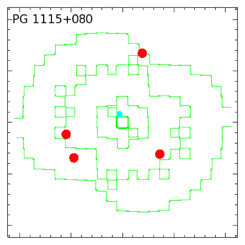
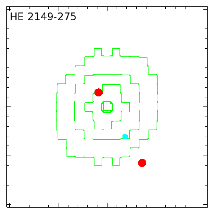
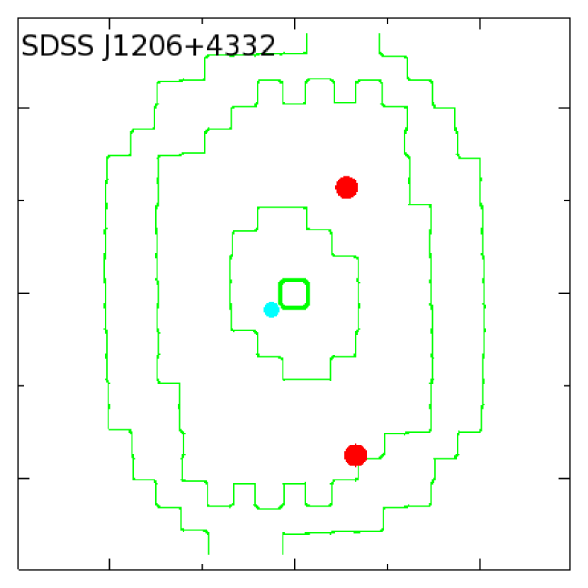
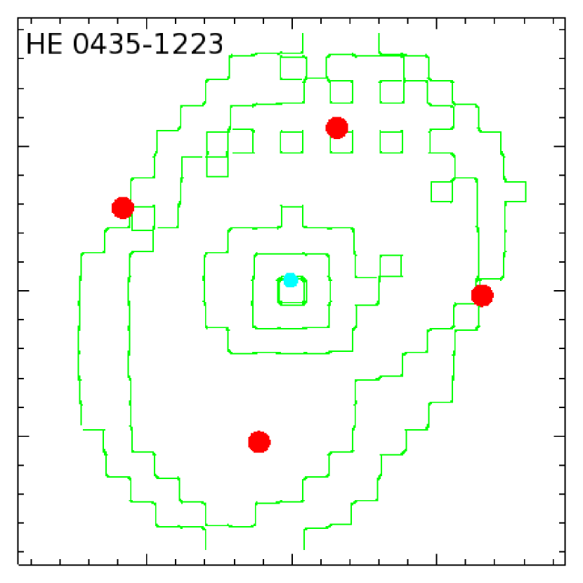
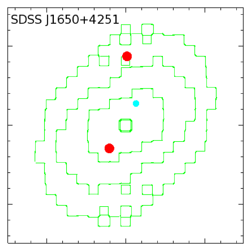
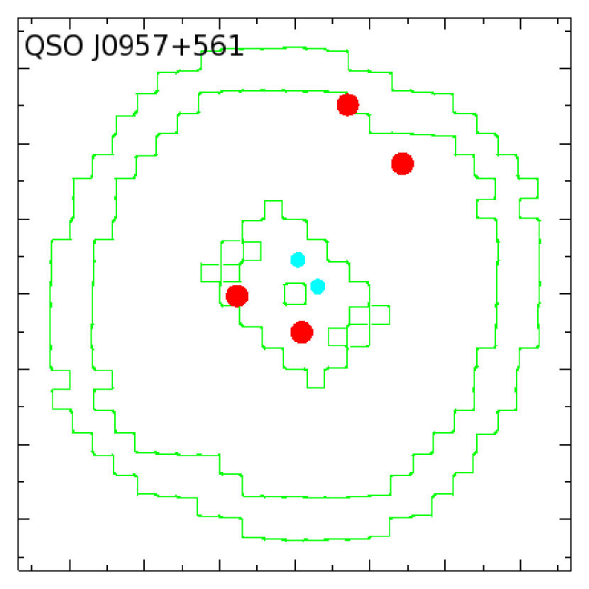
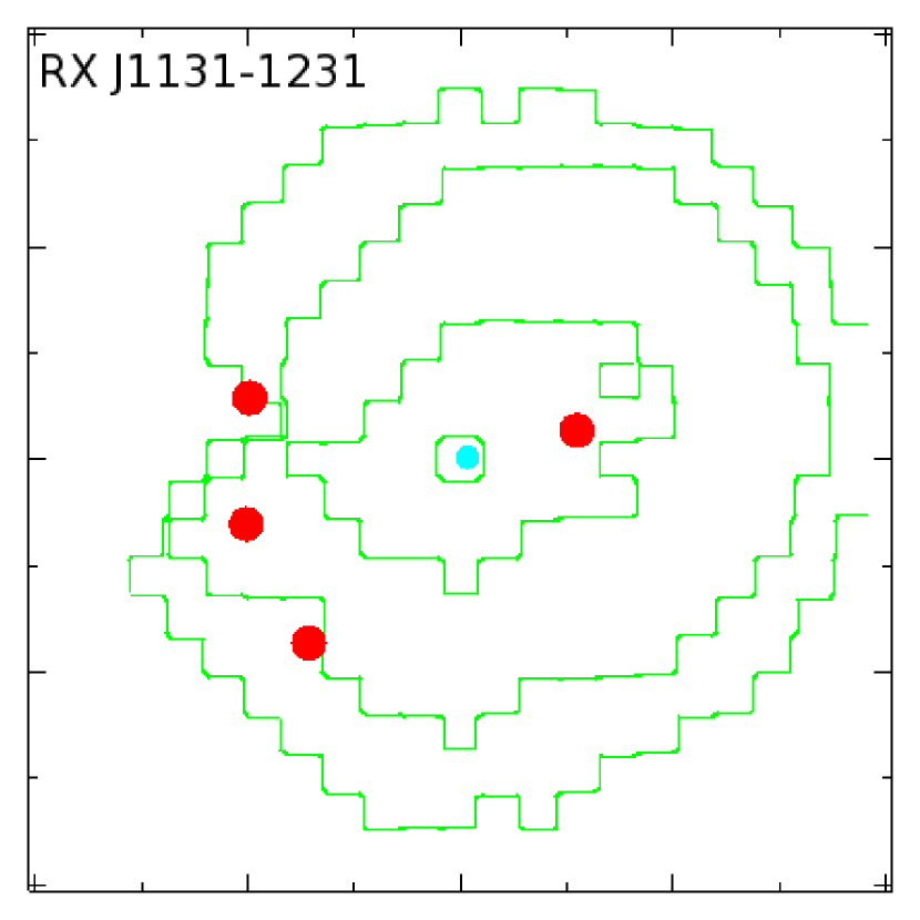
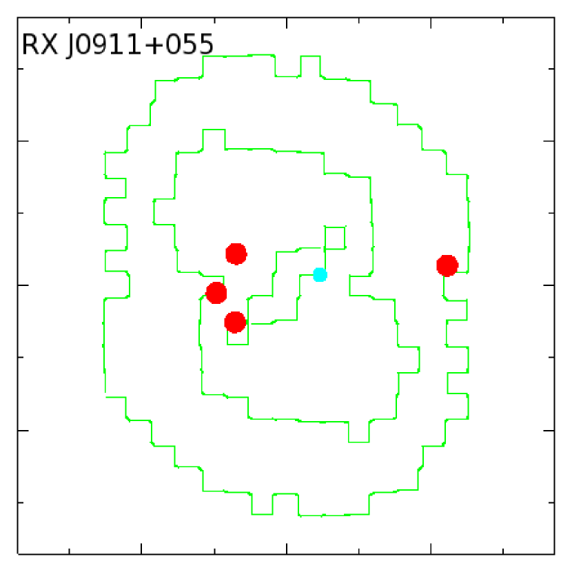
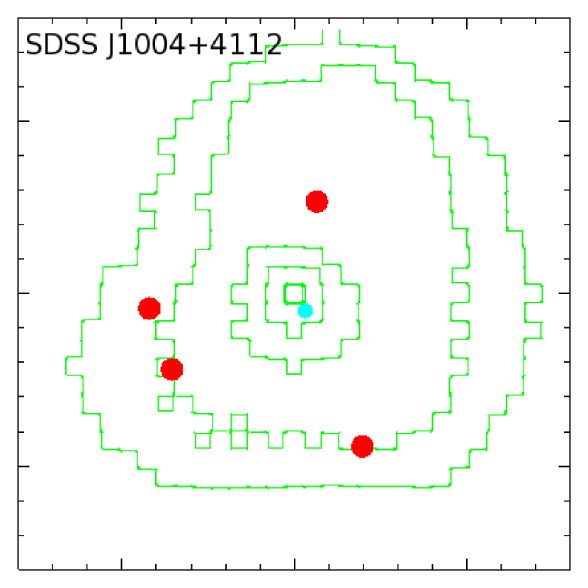
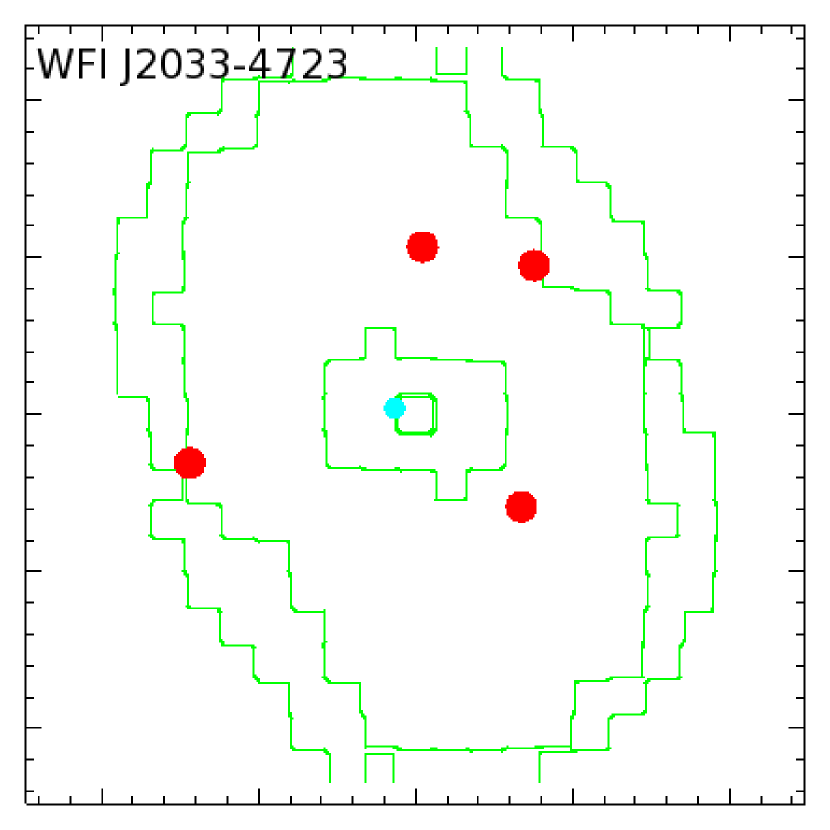
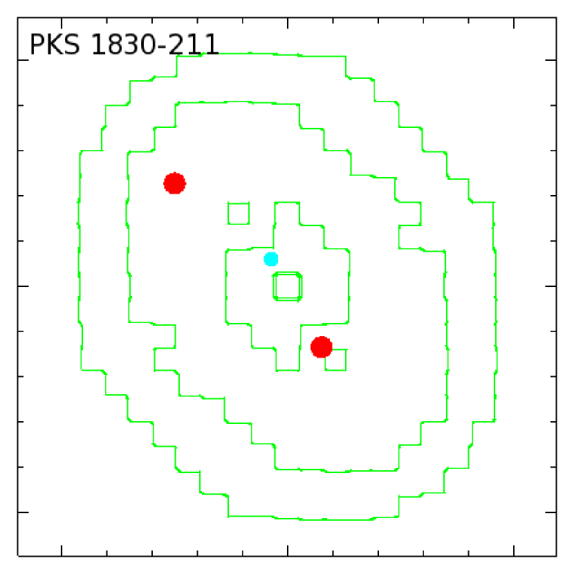
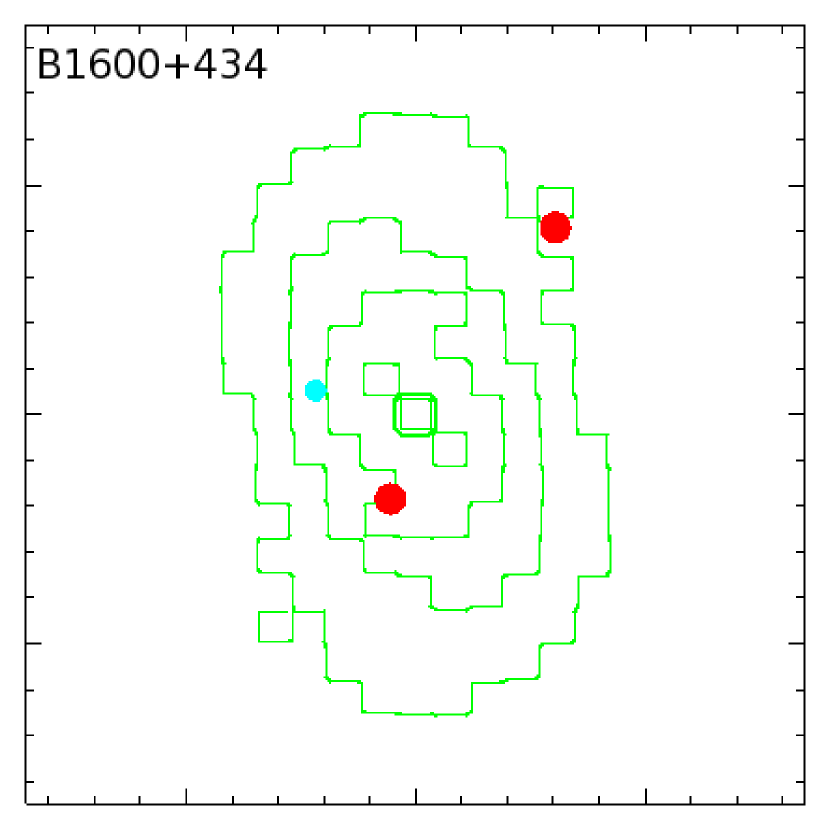
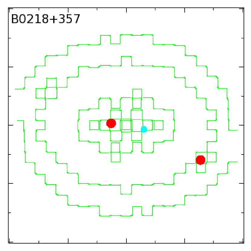
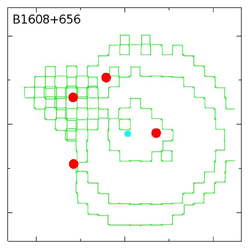
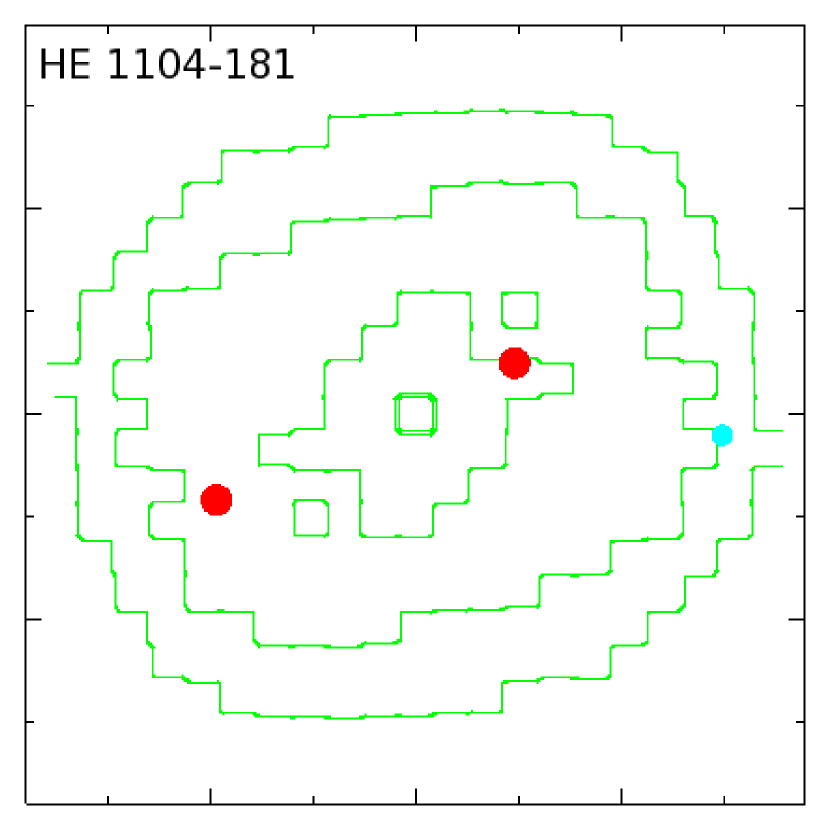
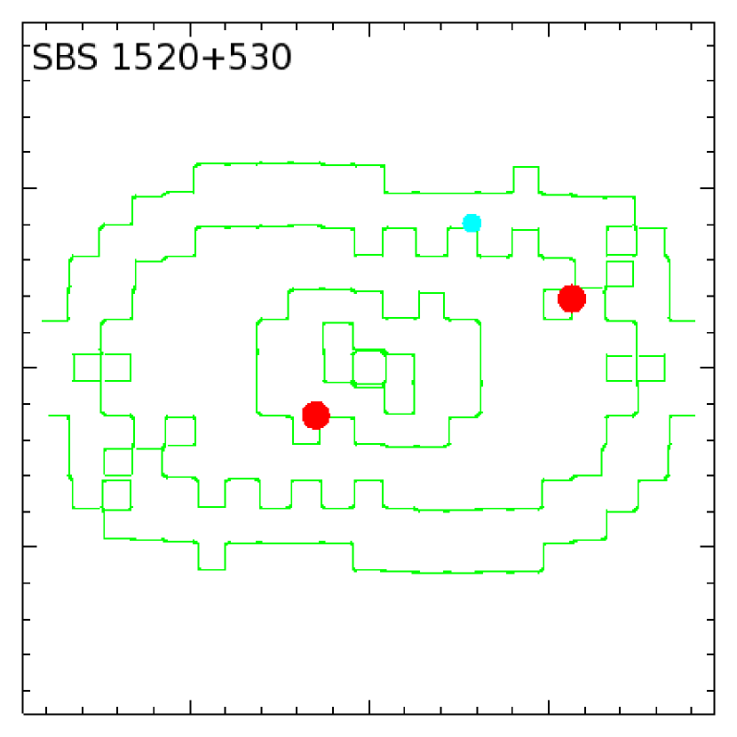
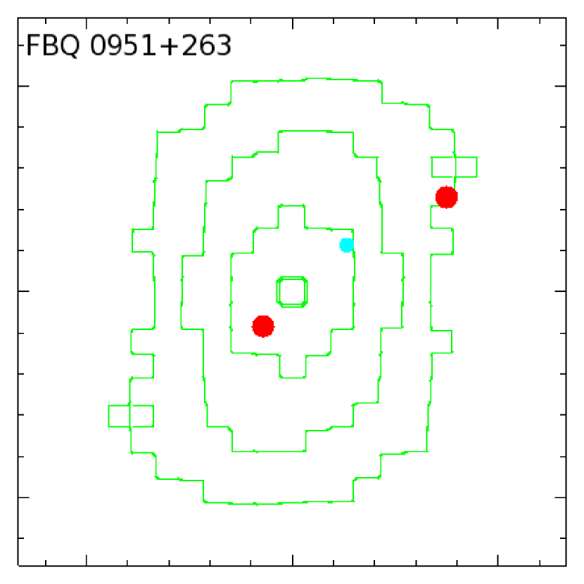
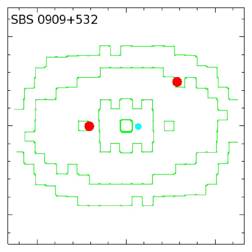
Figure 1: Ensemble of 18 average mass maps of the lenses. The larger tick marks in each panel correspond to $1\farcs 0$. Red and cyan dots represent the positions of the images and the sources respectively. The contours are in logarithmic steps, with critical density corresponding to the third contour from the outside. The systems are grouped according their morphology described in the Section 5.

Table 2: Properties of time-delay lenses

System	$z_{l}$	$z_{s}$	P.A.	Point massa	xb	yb	$\Delta\tau^{c}$	Reference
					($\arcsec$)	($\arcsec$)	(days)
PG 1115+080	0.311	1.722	$-45^{\circ}$	0	0.381	1.344		1, 2, 3, 4
					$-$0.947	$-$0.69	$13.3^{+0.9}_{-1.0}$
					$-$1.096	$-$0.232	0
					0.722	$-$0.617	$11.7^{+1.5}_{-1.6}$
HE 2149-275	0.495	2.030	-	0	0.714	$-$1.150		5, 6, 7
					$-$0.176	0.296	$103\pm 12$
SDSS J1206+4332	0.748	1.789	$50^{\circ}$	0	0.663	$-$1.749		8, 9
					0.566	1.146	$116^{+4}_{-5}$
HE 0435-1223	0.454	1.689	$-65^{\circ}$	0	$-$1.165	0.573		10, 11
					1.311	$-$0.03	$2.1^{+0.78}_{-0.71}$
					0.311	1.126	$6^{+1.07}_{-1.08}$
					$-$0.226	$-$1.041	$8.37^{+1.31}_{-1.37}$
SDSS J1650+4251	0.577	1.547	$80^{\circ}$	0	0.017	0.872		12, 13
					$-$0.206	$-$0.291	$49.5\pm 1.9$
QSO J0957+561	0.356	1.410	$-30^{\circ}$	0	1.408	5.034		14, 15, 16
					0.182	$-$1.018	$422.6\pm 0.6$
					2.860	3.470	0
					$-$1.540	$-$0.050	0
RX J1131-1231	0.295	0.658	$-35^{\circ}$	0	$-$1.984	0.578		17, 3
					$-$1.426	$-$1.73	$1.5^{+2.49}_{-2.02}$
					$-$2.016	$-$0.610	$9.61^{+1.97}_{-1.57}$
					1.096	0.274	$87\pm 8$
RX J0911+055	0.769	2.800	$90^{\circ}$	1	2.226	0.278		18, 19, 20, 21
					$-$0.968	$-$0.105	$146\pm 8$
					$-$0.709	$-$0.507	0
					$-$0.696	0.439	0
SDSS J1004+4112	0.680	1.734	$90^{\circ}$	0	3.943	$-$8.868		5, 22, 23, 24
					$-$8.412	$-$0.86	$821.6\pm 2.1$
					$-$7.095	$-$4.389	$40.6\pm 1.8$
					1.303	5.327	0
WFI J2033-4723	0.661	1.660	$0^{\circ}$	0	$-$1.439	$-$0.311		25, 26, 27
					0.756	0.949	$35.5\pm 1.4$
					0.044	1.068	0
					0.674	$-$0.5891	$27.1^{+4.1}_{-2.3}$
PKS 1830-211	0.885	2.507	-	0	$-$0.498	0.456		28, 29, 30, 31
					0.151	$-$0.268	$26^{+4}_{-5}$
B1600+434	0.410	1.590	$90^{\circ}$	1	0.610	0.814		5, 32, 33, 34
					$-$0.110	$-$0.369	$51\pm 4$
B0218+357	0.685	0.944	-	0	0.250	$-$0.119		35, 36, 37, 38
					$-$0.052	0.007	$10.1^{+1.5}_{-1.6}$
B1608+656	0.630	1.394	-	1	$-$1.155	$-$0.896		39, 40, 41, 42
					$-$0.419	1.059	$31.5\pm 1.5$
					$-$1.165	0.610	0
					0.714	$-$0.197	$41\pm 1.5$
HE 1104-181	0.729	2.319	-	2	$-$1.936	$-$0.832		43, 44, 45
					0.965	0.5	$152.2^{+2.8}_{-3.0}$
SBS 1520+530	0.761	1.855	-	1	1.130	0.387		46, 47, 48, 49
					$-$0.296	$-$0.265	$130\pm 3$
FBQ J0951+263	0.24	1.246	-	0	0.750	0.459		50, 51
					$-$0.142	$-$0.169	$16\pm 2$
SBS 0909+532	0.830	1.376	-	0	0.572	0.494		5, 52, 53
					$-$0.415	$-$0.004	$45^{+1}_{-11}$
B1422+231	0.339	3.62	$10^{\circ}$	0	1.014	$-$0.168		54, 55, 3
					0.291	0.900	$7.6\pm 2.5$
					0.680	0.580	$1.5\pm 1.4$
					$-$0.271	$-$0.222	0

References. — (1) Morgan et al. (2008); (2) Barkana (1997); (3) Tonry (1998); (4) Weymann et al. (1980); (5) CASTLES; (6) Burud et al. (2002a); (7) Wisotzki et al. (1996); (8) Paraficz et al. (2009); (9) Oguri et al. (2005); (10) Kochanek et al. (2006); (11) Morgan et al. (2005); (12) Morgan et al. (2003); (13) Vuissoz et al. (2007); (14) Bernstein & Fischer (1999); (15) Oscoz et al. (2001); (16) Falco et al. (1997); (17) Claeskens et al. (2006); (18) Burud et al. (1998); (19) Hjorth et al. (2002); (20) Kneib et al. (2000); (21) Bade et al. (1997); (22) Fohlmeister et al. (2008); (23) Inada et al. (2003); (24) Williams & Saha (2004); (25) Vuissoz et al. (2008); (26) Eigenbrod et al. (2006); (27) Morgan et al. (2004); (28) Meylan et al. (2005); (29) Lovell et al. (1998); (30) Chengalur et al. (1999); (31) Lidman et al. (1999); (32) Burud et al. (2000); (33) Jaunsen & Hjorth (1997); (34) Jackson et al. (1995); (35) Wucknitz et al. (2004); (36) Cohen et al. (2000); (37) Browne et al. (1993); Carilli et al. (1993); (38) Cohen et al. (2003); (39) Koopmans et al. (2003); (40) Fassnacht et al. (2002); (41) Myers et al. (1995); (42) Fassnacht et al. (1996); (43) Poindexter et al. (2007); (44) Lidman et al. (2000); (45) Wisotzki et al. (1993); (46) Faure et al. (2002); (47) Burud et al. (2002b); (48) Auger et al. (2008); (49) Chavushyan et al. (1997); (50) Jakobsson et al. (2005); (51) White et al. (2000); (52) Ullán et al. (2005); (53) Lubin et al. (2000); (54) Raychaudhury et al. (2003); (55) Patnaik & Narasimha (2001);

(Oguri, 2007) and 10 lenses (Saha et al., 2006). The $H_{0}$ distribution of the samples of 10 and 15 lenses are slightly different than the original results of Oguri (2007) and Saha et al. (2006). Oguri (2007) used 16 lensed quasar systems (40 image pairs) to constrain the Hubble constant. For each image pair, he computed the likelihood as a function of the Hubble constant. He then computed the effective $\chi^{2}$ by summing up the logarithm of the likelihoods. The first summation runs over lens systems, whereas the second summation runs over image pairs for each lens system. He derived the best-fit value and its error of Hubble constant in the standard way using a goodness-of-fit parameter.

Figure 2: Histogram of the ensembles of $H_{0}$ values estimated from 18 lensing systems. We have assumed $\Omega_{\Lambda}=0.7$ and $\Omega_{m}=0.3$.

The difference with Oguri (2007) is mainly due to use of different modeling method and a different statistical and modeling approach to obtain $H_{0}$. In the case of Saha et al. (2006) the method is identical and the difference comes from the use of other/newer data, and the use of different rules for constraining shear, adding secondary lenses, etc. Using the Saha et al. (2006) sample of 10 lenses we have obtained $H_{0}=63_{-5}^{+6}$ $\rm{km}$ $\rm{s}^{-1}\rm{Mpc}^{-1}$ and using the Oguri (2007) sample of 16 lenses (minus B1422+231), we got $H_{0}=66_{-7}^{+5}$ $\rm{km}$ $\rm{s}^{-1}\rm{Mpc}^{-1}$.

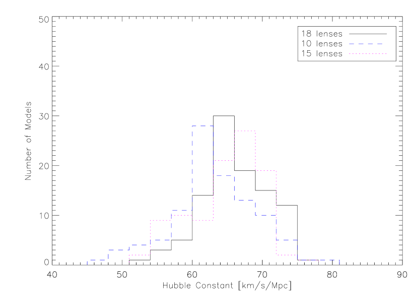
Figure 3: Comparison of the three histograms of the ensembles of $H_{0}$ values. Histogram plotted with the solid line represents our results for 18 systems; the dashed line represents the results of 10 lenses (Saha et al., 2006) and the dotted line is a result of 16 lenses (Oguri, 2007). All calculations are done for a flat Universe with $\Omega_{\Lambda}=0.7$ and $\Omega_{m}=0.3$.

5 ’Elliptical’ sample

The strongest degeneracy in lens modeling is the so-called mass-sheat degeneracy between time delays and the steepness of the mass profile. This degeneracy causes that without change in the images position, we can change the steepness of the mass profile, hence, the resulting $H_{0}$. Thus, if the steepness and $\Delta\tau$ are known, $H_{0}$ is well constrained, although the time delays are also influenced by other more complicated degeneracies involving details of the shape of the lens but these effects are secondary (Saha & Williams, 2006).

In our sample of 18 systems we have galaxies with a variety of steepness. Without detailed observations the profile steepness of each lens is not known, except possibly for elliptical galaxies.

Several studies have shown that elliptical galaxies may be considered as approximately isothermal $\rho\propto r^{-2}$ (Koopmans et al., 2006; Oguri, 2007; Koopmans et al., 2009; Gerhard et al., 2001). Hence, by selecting from our 18 system only elliptical galaxies we expect to get a uniform sample with known slopes of mass profiles.

We have selected five systems that are relatively isolated, elliptical galaxies: PG 1115+080 (Impey et al., 1998), HE 2149-275 (Lopez et al., 1998), SDSS J1206+4332 (Paraficz et al., 2009), HE 0435-1223 (Kochanek et al., 2006) and SDSS J1650+4251 (Vuissoz et al., 2007; Morgan et al., 2003).

Five other lenses were also found to be elliptical but a cluster or group to which they belong has strong influence on the lensing system, thus it is difficult to model them: QSO 0957+561 (Oscoz et al., 1997; Bernstein & Fischer, 1999); RX J1131-1231 (Claeskens et al., 2006); RX J0911+055 (Kneib et al., 2000), SDSS J1004+4112 (Sharon et al., 2005) and WFI J2033-4723 (Eigenbrod et al., 2006),

Three of the lenses are most probably spiral galaxies: PKS 1830-211 is a face-on spiral galaxy (Winn et al., 2002), B1600+434 is a spiral galaxy with a companion (Jaunsen & Hjorth, 1997) and B0218+357 is an isolated spiral galaxy (Koopmans & CLASS, 2001).

The remaining five systems were not included into the ’elliptical’ sample due to various other issues: B1608+656 has two lensing galaxies inside the Einstein ring; HE 1104+180 has little starlight, suggesting a dark matter dominated lens (Poindexter et al., 2007; Vuissoz et al., 2008); SBS 1520+530 has a steeper than isothermal slope, probably due to mergers (Auger et al., 2008); FBQ 0951+263 is a complicated system which is hard to model (Peng et al., 2006); SBS 0909+532 is probably early-type (Lehár et al., 2000) but according Motta et al. (2002) is not very typical due to lots of dust.

Using the sample of five elliptical galaxies and constraining the steepness of their mass profiles to be $\alpha_{min}=1.8$ and $\alpha_{max}=2.2$ we have run the PixeLens simultaneous modeling. The sample of 5 lensing systems gives us a Hubble constant estimation $H_{0}=79_{-3}^{+2}$ $\rm{km}$ $\rm{s}^{-1}\rm{Mpc}^{-1}$ at 68% confidence and $H_{0}=79_{-4}^{+3}$ $\rm{km}$ $\rm{s}^{-1}\rm{Mpc}^{-1}$ at 90% confidence. We have also combined the 5 constrained systems with the rest of the unconstrained sample to perform simultaneous modeling and obtained very well determined Hubble constant $H_{0}=76\pm 3$ $\rm{km}$ $\rm{s}^{-1}\rm{Mpc}^{-1}$ at 68% confidence and $H_{0}=76\pm 5$ $\rm{km}$ $\rm{s}^{-1}\rm{Mpc}^{-1}$ at 90% confidence. The results are presented in Figure 4.

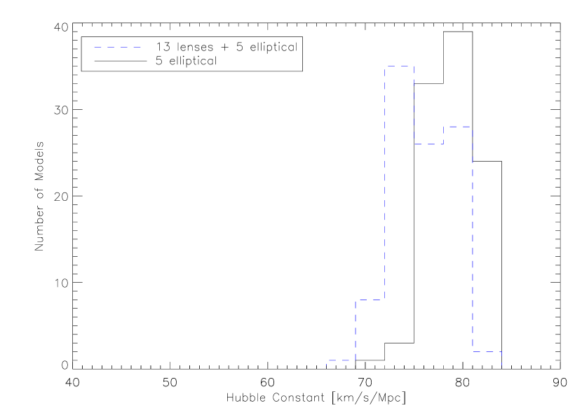
Figure 4: Histogram of the distribution of $H_{0}$ values for the selected sample of 5 elliptical galaxies having constrained steepness of mass profiles in the range 1.8–2.2 (solid line) and the selected elliptical sample combined with the rest of the systems (dashed line). All calculations are done for a flat Universe with $\Omega_{\Lambda}=0.7$ and $\Omega_{m}=0.3$.

6 Conclusions

Non-parametric modeling using PixeLens was applied to an ensemble of 18 lenses to determine a new value for the Hubble constant. We have obtained $H_{0}=66_{-4}^{+6}$ $\rm{km}$ $\rm{s}^{-1}\rm{Mpc}^{-1}$ for a flat Universe with $\Omega_{\Lambda}=0.7$, $\Omega_{m}=0.3$. We have also compared our results with the two previous attempts to estimate $H_{0}$ from time delays (Saha et al., 2006; Oguri, 2007) (Fig. 3).

Our additional result was based on studies of a selected sample of five lensing galaxies that have mass profiles close to $\rho\propto r^{-2}$. The Hubble constant recovered using the selected sample of elliptical galaxies combined with the rest of the systems is $H_{0}=76_{-3}^{+3}$ $\rm{km}$ $\rm{s}^{-1}\rm{Mpc}^{-1}$.

The gravitational lensing method that constrains $H_{0}$ has difficulties due to a couple of degeneracies between mass and time delay. The major degeneracy, the mass-sheet degeneracy, as we have shown, can be addressed by a careful choice of galaxies and the others partially by a combined, pixelated analysis of a large sample of lenses. Pixelated lens modeling provides insight into the structure of galaxies and the distribution of dark matter which together with precise measurements of time delays gives a reliable cosmological method.

Lensing can already determine the Hubble constant approaching the accuracy level of other leading measurements. Nevertheless, still more observation are needed. Future data with precise time delay measurements and better lens models will give even better constraints on $H_{0}$, perhaps turning lensing into a very competitive method.

References

- Auger et al. (2008) Auger, M. W., Fassnacht, C. D., Wong, K. C., Thompson, D., Matthews, K., & Soifer, B. T. 2008, ApJ, 673, 778
- Bade et al. (1997) Bade, N., Siebert, J., Lopez, S., Voges, W., & Reimers, D. 1997, A&A, 317, L13
- Barkana (1997) Barkana, R. 1997, ApJ, 489, 21
- Bernstein & Fischer (1999) Bernstein, G., & Fischer, P. 1999, AJ, 118, 14
- Branch et al. (1996) Branch, D., Fisher, A., Baron, E., & Nugent, P. 1996, ApJ, 470, L7+
- Browne et al. (1993) Browne, I. W. A., Patnaik, A. R., Walsh, D., & Wilkinson, P. N. 1993, MNRAS, 263, L32+
- Burud et al. (1998) Burud, I., et al. 1998, ApJ, 501, L5+
- Burud et al. (2000) —. 2000, ApJ, 544, 117
- Burud et al. (2002a) —. 2002a, A&A, 383, 71
- Burud et al. (2002b) —. 2002b, A&A, 391, 481
- Carilli et al. (1993) Carilli, C. L., Rupen, M. P., & Yanny, B. 1993, ApJ, 412, L59
- Chavushyan et al. (1997) Chavushyan, V. H., Vlasyuk, V. V., Stepanian, J. A., & Erastova, L. K. 1997, A&A, 318, L67
- Chengalur et al. (1999) Chengalur, J. N., de Bruyn, A. G., & Narasimha, D. 1999, A&A, 343, L79
- Claeskens et al. (2006) Claeskens, J.-F., Sluse, D., Riaud, P., & Surdej, J. 2006, A&A, 451, 865
- Cohen et al. (2000) Cohen, A. S., Hewitt, J. N., Moore, C. B., & Haarsma, D. B. 2000, ApJ, 545, 578
- Cohen et al. (2003) Cohen, J. G., Lawrence, C. R., & Blandford, R. D. 2003, ApJ, 583, 67
- Coles (2008) Coles, J. 2008, ApJ, 679, 17
- Dalal & Kochanek (2002) Dalal, N., & Kochanek, C. S. 2002, ApJ, 572, 25
- Eigenbrod et al. (2006) Eigenbrod, A., Courbin, F., Meylan, G., Vuissoz, C., & Magain, P. 2006, A&A, 451, 759
- Elíasdóttir et al. (2006) Elíasdóttir, Á., Hjorth, J., Toft, S., Burud, I., & Paraficz, D. 2006, ApJS, 166, 443
- Falco et al. (1997) Falco, E. E., Shapiro, I. I., Moustakas, L. A., & Davis, M. 1997, ApJ, 484, 70
- Fassnacht et al. (1996) Fassnacht, C. D., Womble, D. S., Neugebauer, G., Browne, I. W. A., Readhead, A. C. S., Matthews, K., & Pearson, T. J. 1996, ApJ, 460, L103+
- Fassnacht et al. (2002) Fassnacht, C. D., Xanthopoulos, E., Koopmans, L. V. E., & Rusin, D. 2002, ApJ, 581, 823
- Faure et al. (2002) Faure, C., Courbin, F., Kneib, J. P., Alloin, D., Bolzonella, M., & Burud, I. 2002, A&A, 386, 69
- Fohlmeister et al. (2008) Fohlmeister, J., Kochanek, C. S., Falco, E. E., Morgan, C. W., & Wambsganss, J. 2008, ApJ, 676, 761
- Freedman et al. (2001) Freedman, W. L., et al. 2001, ApJ, 553, 47
- Gerhard et al. (2001) Gerhard, O., Kronawitter, A., Saglia, R. P., & Bender, R. 2001, AJ, 121, 1936
- Hjorth et al. (2002) Hjorth, J., et al. 2002, ApJ, 572, L11
- Impey et al. (1998) Impey, C. D., Falco, E. E., Kochanek, C. S., Lehár, J., McLeod, B. A., Rix, H.-W., Peng, C. Y., & Keeton, C. R. 1998, ApJ, 509, 551
- Inada et al. (2003) Inada, N., et al. 2003, Nature, 426, 810
- Jackson et al. (1995) Jackson, N., et al. 1995, MNRAS, 274, L25
- Jakobsson et al. (2005) Jakobsson, P., Hjorth, J., Burud, I., Letawe, G., Lidman, C., & Courbin, F. 2005, A&A, 431, 103
- Jaunsen & Hjorth (1997) Jaunsen, A. O., & Hjorth, J. 1997, A&A, 317, L39
- Jones et al. (2005) Jones, M. E., et al. 2005, MNRAS, 357, 518
- Kneib et al. (2000) Kneib, J.-P., Cohen, J. G., & Hjorth, J. 2000, ApJ, 544, L35
- Kochanek et al. (2006) Kochanek, C. S., Morgan, N. D., Falco, E. E., McLeod, B. A., Winn, J. N., Dembicky, J., & Ketzeback, B. 2006, ApJ, 640, 47
- Komatsu et al. (2009) Komatsu, E., et al. 2009, ApJS, 180, 330
- Koopmans & CLASS (2001) Koopmans, L. V. E., & CLASS. 2001, Publications of the Astronomical Society of Australia, 18, 179
- Koopmans et al. (2006) Koopmans, L. V. E., Treu, T., Bolton, A. S., Burles, S., & Moustakas, L. A. 2006, ApJ, 649, 599
- Koopmans et al. (2003) Koopmans, L. V. E., Treu, T., Fassnacht, C. D., Blandford, R. D., & Surpi, G. 2003, ApJ, 599, 70
- Koopmans et al. (2009) Koopmans, L. V. E., et al. 2009, ArXiv:0906.1349
- Lehár et al. (2000) Lehár, J., et al. 2000, ApJ, 536, 584
- Lidman et al. (2000) Lidman, C., Courbin, F., Kneib, J.-P., Golse, G., Castander, F., & Soucail, G. 2000, A&A, 364, L62
- Lidman et al. (1999) Lidman, C., Courbin, F., Meylan, G., Broadhurst, T., Frye, B., & Welch, W. J. W. 1999, ApJ, 514, L57
- Lopez et al. (1998) Lopez, S., Wucknitz, O., & Wisotzki, L. 1998, A&A, 339, L13
- Lovell et al. (1998) Lovell, J. E. J., Jauncey, D. L., Reynolds, J. E., Wieringa, M. H., King, E. A., Tzioumis, A. K., McCulloch, P. M., & Edwards, P. G. 1998, ApJ, 508, L51
- Lubin et al. (2000) Lubin, L. M., Fassnacht, C. D., Readhead, A. C. S., Blandford, R. D., & Kundić, T. 2000, AJ, 119, 451
- Meylan et al. (2005) Meylan, G., Courbin, F., Lidman, C., Kneib, J.-P., & Tacconi-Garman, L. E. 2005, A&A, 438, L37
- Morgan et al. (2008) Morgan, C. W., Kochanek, C. S., Dai, X., Morgan, N. D., & Falco, E. E. 2008, ApJ, 689, 755
- Morgan et al. (2004) Morgan, N. D., Caldwell, J. A. R., Schechter, P. L., Dressler, A., Egami, E., & Rix, H.-W. 2004, AJ, 127, 2617
- Morgan et al. (2005) Morgan, N. D., Kochanek, C. S., Pevunova, O., & Schechter, P. L. 2005, AJ, 129, 2531
- Morgan et al. (2003) Morgan, N. D., Snyder, J. A., & Reens, L. H. 2003, AJ, 126, 2145
- Motta et al. (2002) Motta, V., et al. 2002, ApJ, 574, 719
- Myers et al. (1995) Myers, S. T., et al. 1995, ApJ, 447, L5+
- Oguri (2007) Oguri, M. 2007, ApJ, 660, 1
- Oguri et al. (2005) Oguri, M., et al. 2005, ApJ, 622, 106
- Oscoz et al. (1997) Oscoz, A., Mediavilla, E., Goicoechea, L. J., Serra-Ricart, M., & Buitrago, J. 1997, ApJ, 479, L89+
- Oscoz et al. (2001) Oscoz, A., et al. 2001, ApJ, 552, 81
- Paraficz et al. (2006) Paraficz, D., Hjorth, J., Burud, I., Jakobsson, P., & Elíasdóttir, Á. 2006, A&A, 455, L1
- Paraficz et al. (2009) Paraficz, D., Hjorth, J., & Elíasdóttir, Á. 2009, A&A, 499, 395
- Patnaik & Narasimha (2001) Patnaik, A. R., & Narasimha, D. 2001, MNRAS, 326, 1403
- Peng et al. (2006) Peng, C. Y., Impey, C. D., Rix, H.-W., Kochanek, C. S., Keeton, C. R., Falco, E. E., Lehár, J., & McLeod, B. A. 2006, ApJ, 649, 616
- Poindexter et al. (2007) Poindexter, S., Morgan, N., Kochanek, C. S., & Falco, E. E. 2007, ApJ, 660, 146
- Raychaudhury et al. (2003) Raychaudhury, S., Saha, P., & Williams, L. L. R. 2003, AJ, 126, 29
- Refsdal (1964) Refsdal, S. 1964, MNRAS, 128, 307
- Riess et al. (2009) Riess, A. G., et al. 2009, ApJ, 699, 539
- Saha et al. (2006) Saha, P., Coles, J., Macciò, A. V., & Williams, L. L. R. 2006, ApJ, 650, L17
- Saha & Williams (2004) Saha, P., & Williams, L. L. R. 2004, AJ, 127, 2604
- Saha & Williams (2006) —. 2006, ApJ, 653, 936
- Sandage et al. (2006) Sandage, A., Tammann, G. A., Saha, A., Reindl, B., Macchetto, F. D., & Panagia, N. 2006, ApJ, 653, 843
- Sharon et al. (2005) Sharon, K., et al. 2005, ApJ, 629, L73
- Spergel et al. (2007) Spergel, D. N., et al. 2007, ApJS, 170, 377
- Suyu et al. (2009) Suyu, S. H., Marshall, P. J., Auger, M. W., Hilbert, S., Blandford, R. D., Koopmans, L. V. E., Fassnacht, C. D., & Treu, T. 2009, ArXiv e-prints
- Tonry (1998) Tonry, J. L. 1998, AJ, 115, 1
- Ullán et al. (2005) Ullán, A., Goicoechea, L. J., Gil-Merino, R., Serra-Ricart, M., Muñoz, J. A., Mediavilla, E., González-Cadelo, J., & Oscoz, A. 2005, in IAU Symposium, Vol. 225, Gravitational Lensing Impact on Cosmology, ed. Y. Mellier & G. Meylan, 305–310
- Vuissoz et al. (2007) Vuissoz, C., et al. 2007, A&A, 464, 845
- Vuissoz et al. (2008) —. 2008, A&A, 488, 481
- Weymann et al. (1980) Weymann, R. J., et al. 1980, Nature, 285, 641
- White et al. (2000) White, R. L., et al. 2000, ApJS, 126, 133
- Williams & Saha (2004) Williams, L. L. R., & Saha, P. 2004, AJ, 128, 2631
- Winn et al. (2002) Winn, J. N., Kochanek, C. S., McLeod, B. A., Falco, E. E., Impey, C. D., & Rix, H.-W. 2002, ApJ, 575, 103
- Wisotzki et al. (1993) Wisotzki, L., Koehler, T., Kayser, R., & Reimers, D. 1993, A&A, 278, L15
- Wisotzki et al. (1996) Wisotzki, L., Koehler, T., Lopez, S., & Reimers, D. 1996, A&A, 315, L405+
- Wucknitz et al. (2004) Wucknitz, O., Biggs, A. D., & Browne, I. W. A. 2004, MNRAS, 349, 14