Anisotropy of Solar Wind Turbulence between Ion and Electron Scales
Abstract
The anisotropy of turbulence in the fast solar wind, between the ion and electron gyroscales, is directly observed using a multispacecraft analysis technique. Second order structure functions are calculated at different angles to the local magnetic field, for magnetic fluctuations both perpendicular and parallel to the mean field. In both components, the structure function value at large angles to the field is greater than at small angles : in the perpendicular component and in the parallel component , implying spatially anisotropic fluctuations, . The spectral index of the perpendicular component is at large angles and at small angles, in broad agreement with critically balanced whistler and kinetic Alfvén wave predictions. For the parallel component, however, it is shallower than , which is considerably less steep than predicted for a kinetic Alfvén wave cascade.
pacs:
94.05.Lk, 52.35.Ra, 96.60.Vg, 96.50.BhIntroduction.—Solar wind turbulence has been studied for many decades (e.g., Goldstein et al. (1995) and references therein) but a number of fundamental aspects of it remain poorly understood. This Letter will address one of these, the nature of the turbulent fluctuations at small scales, using a recently developed multispacecraft analysis technique.
Turbulence is usually modeled as a cascade of energy, with injection at large scales and dissipation at small scales. In the solar wind, the injected energy is thought to originate from the observed large scale Alfvén waves Belcher and Davis (1971). For scales between the effective outer scale and the ion gyroradius, termed the inertial range, a cascade of Alfvénic fluctuations Iroshnikov (1964); Kraichnan (1965); Goldreich and Sridhar (1995); Boldyrev (2006); Schekochihin et al. (2009) is often invoked to explain the observed power spectra Coleman (1968); Matthaeus and Goldstein (1982); Bale et al. (2005); Podesta et al. (2007). One aspect of recent investigation in the solar wind inertial range, relevant to this study, is anisotropy with respect to the magnetic field. It has been shown that both power and scalings vary with respect to the local magnetic field direction Bieber et al. (1996); Horbury et al. (2008); Podesta (2009); Osman and Horbury (2009); Wicks et al. (2010), in a way consistent with critical balance theories Goldreich and Sridhar (1995); Boldyrev (2006).
At smaller scales, close to the ion gyroradius, the magnetic field power spectrum steepens (e.g., Leamon et al. (1998); Smith et al. (2006)). This is commonly termed the dissipation range, although is sometimes called the dispersion range (e.g., Stawicki et al. (2001)), and is where kinetic effects become important. Recent measurements of the magnetic field spectral index in this range are between and Alexandrova et al. (2008a); Sahraoui et al. (2009); Kiyani et al. (2009); Alexandrova et al. (2009), although larger variation was seen in an earlier survey Smith et al. (2006). A further steepening in the spectrum near the electron gyroscale has also been observed Sahraoui et al. (2009); Alexandrova et al. (2009). In this study, we investigate between the ion and electron scales. Two popular suggestions for the types of fluctuations in this range are kinetic Alfvén waves (KAWs) Leamon et al. (1998); Bale et al. (2005); Schekochihin et al. (2009); Sahraoui et al. (2009); Howes and Quataert (2010) and whistler waves Stawicki et al. (2001); Biskamp et al. (1996). It has been suggested Cho and Lazarian (2004); Schekochihin et al. (2009) that, like some inertial range theories Goldreich and Sridhar (1995); Boldyrev (2006), the fluctuations are critically balanced, which would imply a spectral index of in the perpendicular direction and in the parallel direction.
In this Letter, the first multispacecraft structure function measurements in the solar wind at scales below the ion gyroscale are presented. The variance, power, and spectral index anisotropy in the magnetic field components parallel and perpendicular to the field are calculated. This provides a direct test of existing theories and a guide for new ones.
Data set.—We use an interval of data from the Cluster mission Escoubet et al. (2001), in which the four spacecraft are in the fast solar wind with a separation 100 km. The interval parameters are given in Table 1 and are from the FGM Balogh et al. (2001), CIS Rème et al. (2001), and PEACE Johnstone et al. (1997) instruments. No effects of Earth’s foreshock are present, and the interval lies in the stable region of the parameter space for pressure anisotropy instabilities (e.g., Bale et al. (2009)).
| Date | Time | |||||||||||||
|---|---|---|---|---|---|---|---|---|---|---|---|---|---|---|
| (dd/mm/yy) | (UT) | (km s-1) | (cm-3) | (km s-1) | (eV) | (eV) | (eV) | (eV) | (km) | (km) | (km) | (km) | ||
| 11/02/02 | 19:19–20:29 |
For analyzing the fluctuations between ion and electron scales, high frequency data, 1 Hz, is needed. In this study, a measurement of the local magnetic field direction is used, requiring data valid at both low and high frequencies. The STAFF instrument Cornilleau-Wehrlin et al. (2003) has a high frequency search coil magnetometer, which provides a time series valid in the approximate range 0.6–10 Hz. We combine this with the FGM data, which is valid up to 1 Hz in the solar wind.
The combining procedure is based on the method in Appendix A of Ref. Alexandrova et al. (2004). First, the high frequency (22 Hz) FGM data are interpolated onto the times of the STAFF data (25 Hz). A wavelet transform is then applied to both time series to obtain two sets of wavelet coefficients for each field component. The wavelet coefficients corresponding to the STAFF data above 1 Hz are used to generate a high frequency time series, and those corresponding to the FGM data below 1 Hz are used to generate a low frequency time series. The two time series are then added, resulting in the combined signal.
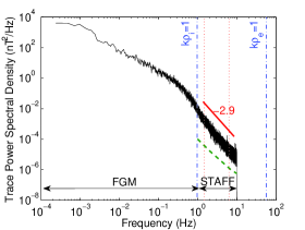
The power spectrum of the combined data is shown in Fig. 1 with the approximate ranges of FGM and STAFF marked. The noise floor of STAFF (from ground and in-flight tests Cornilleau-Wehrlin et al. (2003)) is also shown. The break in the spectrum at 0.4 Hz is the ion scale spectral break point at the end of the inertial range, and is not due to the data merging. For this interval, the isotropic spectral index for the range of scales we study is .
Method.—A multispacecraft method is used in which data from the four Cluster spacecraft are combined to produce second order structure functions in different directions to the local magnetic field. It is based on the method of Ref. Osman and Horbury (2009). One benefit of this technique is that a range of sampling angles can be covered simultaneously, enabling short intervals to be used, increasing the likelihood of statistical stationarity.
Compared to the solar wind flow, the four spacecraft are approximately stationary and measure the magnetic field as the solar wind passes by. The measured variations, therefore, are due to both temporal and spatial variations in the plasma. Assuming that the temporal changes happen slowly compared to the flow, each time series can be converted into a spatial cut through the plasma (Taylor’s hypothesis Taylor (1938)). Second order structure functions can then be calculated, defined as , where is the th component of the magnetic field, is the separation vector, and the angular brackets denote an ensemble average over positions .
It is important to consider the application of Taylor’s hypothesis at small scales. In the inertial range, the solar wind speed is usually an order of magnitude larger than the Alfvén speed and, therefore, Taylor’s hypothesis is well satisfied. At smaller scales, the wave phase speed is larger than the Alfvén speed Bale et al. (2005); Sahraoui et al. (2009). It is still lower than the solar wind speed, however, so even if Taylor’s hypothesis is less well satisfied than in the inertial range, it is not an unreasonable assumption. Measurements with an Alfvénic Taylor ratio (as defined in Ref. Osman and Horbury (2009)) greater than 0.25 are discarded.
Axisymmetry about the magnetic field is assumed so that can be split into parallel and perpendicular components, . There is mounting evidence that it is the local magnetic field that orders the fluctuations rather than a global field Cho and Vishniac (2000); Maron and Goldreich (2001); Horbury et al. (2008); Beresnyak and Lazarian (2009); Tessein et al. (2009); i.e., the turbulence is anisotropic with respect to the field at the scale of each fluctuation rather than a much larger scale. Here, the local field is defined as , and its direction is used to define and . The parallel and perpendicular components of for each structure function pair are also defined with respect to .
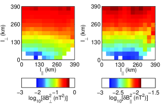
The structure function values obtained from many pairs of magnetic field measurements from all four spacecraft are binned with respect to and and averaged. A minimum number of 200 values per bin is set to ensure reliable results and the binned data for each component are shown in Fig. 2. In both and anisotropy can be seen: the structure function contours are elongated along the local field direction. Similar results have been seen at larger scales in inertial range solar wind correlation functions Osman and Horbury (2007), and in structure functions from MHD Cho and Vishniac (2000) and electron MHD Cho and Lazarian (2004, 2009) simulations.
Instead of Cartesian coordinates, , the data can be binned in polar coordinates, , where is the angle to the local magnetic field (see Fig. 3). Because of the low power, it is possible that the noise floor of STAFF has been reached for the small angle bins in . This can be seen in Fig. 3, in which the lowest value structure function curves appear flatter than the others. Caution, therefore, is advised when interpreting these lowest power measurements.
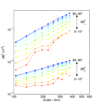
Variance anisotropy.—The ratio of power in the perpendicular component to the parallel component is sometimes referred to as variance anisotropy, (e.g., Hamilton et al. (2008)). From Fig. 3 it can be seen that is about 5% of , which is smaller than average values of previous measurements Leamon et al. (1998); Hamilton et al. (2008). This could be due to statistical variation, or due to the global, rather than local, mean field direction being used in those studies.
The variance anisotropy for KAWs in electron reduced MHD Schekochihin et al. (2009) can be calculated, and for the parameters in Table 1 this prediction is , which is larger than the value observed here. Numerical solutions of linear kinetic theory, however, suggest smaller values of variance anisotropy for KAWs Gary and Smith (2009). These values depend on , propagation angle, and wave number, but are in the range 0.01 to 0.2, which agrees with our result of 0.05.
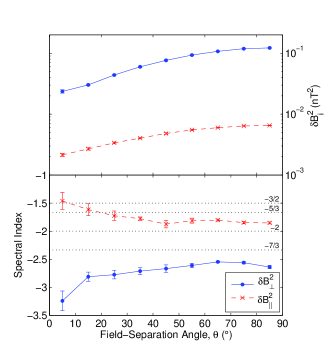
Power anisotropy.—Straight lines (in log-log space) are fitted to the data in Fig. 3 over the range 100–400 km. This is between ion and electron scales, i.e., between and , where . The interpolated values of the structure function at 200 km from these fits are given as a function of in the upper panel of Fig. 4. The error bars are small, comparable to the data point size, and are the standard deviations of the points about the best fit lines.
For both components, the structure function value (“power”) increases with . This is consistent with spatially anisotropic fluctuations, , where and are characteristic parallel and perpendicular wave numbers Chen et al. (2010). One measure of this anisotropy is the ratio of the largest angle bin value to the smallest , which for is . This number is uncertain for , due to the noise issues mentioned above, but has a lower limit of 3.
Some previous studies of the solar wind between ion and electron scales have measured anisotropy using the “slab plus 2D” model Leamon et al. (1998); Hamilton et al. (2008). The large slab fractions obtained are not generally in agreement with this study. In fact, our results are more consistent with other solar wind Narita et al. (2007); Podesta (2009) and magnetosheath Alexandrova et al. (2008b) measurements that demonstrate significant spatial anisotropy at scales smaller than the ion gyroscale.
Spectral index anisotropy.—An important characteristic of turbulence is the spectral index of the power spectrum, . Second order structure function scalings, i.e., gradients , of the straight line fits to the data in Fig. 3, are related to the spectral index by Monin and Yaglom (1975). Using this relationship, the spectral index as a function of angle , for and , is shown in Fig. 4. The error bars are the standard errors on the best fit line gradients.
For , the spectral index varies from around at large angles to at small angles. It should be noted that the steepest spectral index it is possible to measure with this method is (e.g., Monin and Yaglom (1975); Cho and Lazarian (2009)); for steeper spectra, the scaling seen by the two-point second order structure function is , since it is dominated by the smooth variation of the large scale field. At small angles, we observe a spectral index of , indicating that the spectrum in the parallel direction is or steeper. The predictions for a critically balanced whistler or KAW cascade are in the perpendicular direction and in the parallel direction Cho and Lazarian (2004); Schekochihin et al. (2009). Although the spectral indices in Fig. 4 are slightly steeper than the prediction at large values of , the steepening towards small is suggestive of a critically balanced cascade.
The spectral index of varies from at large angles to at small angles. The small angle values may be affected by noise (as discussed previously), but the large angle ones appear not to be, and are significantly shallower than those of . This difference in gradient between the components can also be seen in Fig. 3. For a KAW cascade, is expected to scale in the same way as Schekochihin et al. (2009). The difference observed here, therefore, may be indicating the presence of other modes or a different cascade mechanism. Another possibility for the difference is instability generated fluctuations, although the measured parameters suggest the interval is not unstable to pressure anisotropy instabilities (e.g., Bale et al. (2009)).
Summary and conclusions.—The variance, power, and spectral index anisotropy are measured in the fast solar wind, between the ion and electron gyroscales. The variance anisotropy is significant, with being approximately 5% of . Both magnetic field components display power anisotropy, implying spatially anisotropic fluctuations, . The spectral index of steepens at small angles to the field, which is consistent with a critically balanced cascade of whistlers or KAWs. The spectral indices of are less consistent with the predictions, suggesting that the KAW picture Schekochihin et al. (2009) may be incomplete.
Although we have looked for other data intervals, it is hard to find ones that satisfy the conditions required for this analysis, i.e., 1 h long, away from Earth’s foreshock, with small spacecraft separations and good angular coverage. A larger study is required to determine if the behavior noted here is typical for the solar wind. This may need to wait for a future mission due to the limitations of multispacecraft data currently available.
Acknowledgements.
This work was funded by STFC and the Leverhulme Trust Network for Magnetized Plasma Turbulence. FGM and CIS data were obtained from the Cluster Active Archive. C. C. acknowledges useful conversations with K. Osman, P. Brown, and S. Schwartz.References
- Goldstein et al. (1995) M. L. Goldstein et al., Annu. Rev. Astron. Astrophys. 33, 283 (1995); T. S. Horbury et al., Plasma Phys. Controlled Fusion 47, B703 (2005); R. Bruno and V. Carbone, Living Rev. Solar Phys. 2, 4 (2005).
- Belcher and Davis (1971) J. W. Belcher and L. Davis, Jr., J. Geophys. Res. 76, 3534 (1971).
- Iroshnikov (1964) P. S. Iroshnikov, Soviet Astronomy 7, 566 (1964).
- Kraichnan (1965) R. H. Kraichnan, Phys. Fluids 8, 1385 (1965).
- Goldreich and Sridhar (1995) P. Goldreich and S. Sridhar, Astrophys. J. 438, 763 (1995).
- Boldyrev (2006) S. Boldyrev, Phys. Rev. Lett. 96, 115002 (2006).
- Schekochihin et al. (2009) A. A. Schekochihin et al., Astrophys. J. 182, 310 (2009).
- Coleman (1968) P. J. Coleman, Jr., Astrophys. J. 153, 371 (1968).
- Matthaeus and Goldstein (1982) W. H. Matthaeus and M. L. Goldstein, J. Geophys. Res. 87, 6011 (1982).
- Bale et al. (2005) S. D. Bale et al., Phys. Rev. Lett. 94, 215002 (2005).
- Podesta et al. (2007) J. J. Podesta et al., Astrophys. J. 664, 543 (2007).
- Bieber et al. (1996) J. W. Bieber et al., J. Geophys. Res. 101, 2511 (1996).
- Horbury et al. (2008) T. S. Horbury et al., Phys. Rev. Lett. 101, 175005 (2008).
- Podesta (2009) J. J. Podesta, Astrophys. J. 698, 986 (2009).
- Osman and Horbury (2009) K. T. Osman and T. S. Horbury, Ann. Geophys. 27, 3019 (2009).
- Wicks et al. (2010) R. T. Wicks et al., arXiv:1002.2096v1.
- Leamon et al. (1998) R. J. Leamon et al., J. Geophys. Res. 103, 4775 (1998).
- Smith et al. (2006) C. W. Smith et al., Astrophys. J. 645, L85 (2006).
- Stawicki et al. (2001) O. Stawicki et al., J. Geophys. Res. 106, 8273 (2001).
- Alexandrova et al. (2008a) O. Alexandrova et al., Astrophys. J. 674, 1153 (2008a).
- Sahraoui et al. (2009) F. Sahraoui et al., Phys. Rev. Lett. 102, 231102 (2009).
- Kiyani et al. (2009) K. H. Kiyani et al., Phys. Rev. Lett. 103, 075006 (2009).
- Alexandrova et al. (2009) O. Alexandrova et al., Phys. Rev. Lett. 103, 165003 (2009).
- Howes and Quataert (2010) G. G. Howes and E. Quataert, Astrophys. J. 709, L49 (2010).
- Biskamp et al. (1996) D. Biskamp et al., Phys. Rev. Lett. 76, 1264 (1996); S. Galtier, J. Low Temp. Phys. 145, 59 (2006); W. H. Matthaeus et al., Phys. Rev. Lett. 101, 149501 (2008); S. Saito et al., Phys. Plasmas 15, 102305 (2008).
- Cho and Lazarian (2004) J. Cho and A. Lazarian, Astrophys. J. 615, L41 (2004).
- Escoubet et al. (2001) C. P. Escoubet et al., Ann. Geophys. 19, 1197 (2001).
- Balogh et al. (2001) A. Balogh et al., Ann. Geophys. 19, 1207 (2001).
- Rème et al. (2001) H. Rème et al., Ann. Geophys. 19, 1303 (2001).
- Johnstone et al. (1997) A. D. Johnstone et al., Space Sci. Rev. 79, 351 (1997).
- Bale et al. (2009) S. D. Bale et al., Phys. Rev. Lett. 103, 211101 (2009).
- Cornilleau-Wehrlin et al. (2003) N. Cornilleau-Wehrlin et al., Ann. Geophys. 21, 437 (2003).
- Alexandrova et al. (2004) O. Alexandrova et al., J. Geophys. Res. 109, A05207 (2004).
- Taylor (1938) G. I. Taylor, Proc. R. Soc. A 164, 476 (1938).
- Cho and Vishniac (2000) J. Cho and E. T. Vishniac, Astrophys. J. 539, 273 (2000).
- Maron and Goldreich (2001) J. Maron and P. Goldreich, Astrophys. J. 554, 1175 (2001).
- Beresnyak and Lazarian (2009) A. Beresnyak and A. Lazarian, Astrophys. J. 702, 460 (2009).
- Tessein et al. (2009) J. A. Tessein et al., Astrophys. J. 692, 684 (2009).
- Osman and Horbury (2007) K. T. Osman and T. S. Horbury, Astrophys. J. 654, L103 (2007).
- Cho and Lazarian (2009) J. Cho and A. Lazarian, Astrophys. J. 701, 236 (2009).
- Hamilton et al. (2008) K. Hamilton et al., J. Geophys. Res. 113, A01106 (2008).
- Gary and Smith (2009) S. P. Gary and C. W. Smith, J. Geophys. Res. 114, A12105 (2009).
- Chen et al. (2010) C. H. K. Chen et al., Astrophys. J. 711, L79 (2010).
- Narita et al. (2007) Y. Narita et al., in Proceedings of the 6th Annual International Astrophysical Conference, Oahu, Hawaii, 2007, edited by D. Shaikh and G. P. Zank (AIP, New York, 2007), Vol. 932, pp. 215-220.
- Alexandrova et al. (2008b) O. Alexandrova et al., Ann. Geophys. 26, 3585 (2008b).
- Monin and Yaglom (1975) A. S. Monin and A. M. Yaglom, Statistical Fluid Mechanics, Vol 2 (MIT Press, Cambridge, Mass., 1975).