Testing the Non-universal $Z^{\prime}$ Model in $B_{s}\to\phi\pi^{0}$ Decay

Abstract

The branching ratio and direct CP asymmetry of the decay mode $B_{s}\to\phi\pi^{0}$ have been calculated within the QCD factorization approach in both the standard model (SM) and the non-universal $Z^{\prime}$ model. In the standard model, the CP averaged branching ratio is about $1.3\times 10^{-7}$. Considering the effect of $Z^{\prime}$ boson, we found the branching ratio can be enlarged three times or decreased to one third within the allowed parameter spaces. Furthermore, the direct CP asymmetry could reach $55\%$ with a light $Z^{\prime}$ boson and suitable CKM phase, compared to $25\%$ predicted in the SM. The enhancement of both branching ratio and CP asymmetry cannot be realized at the same parameter spaces, thus, if this decay mode is measured in the upcoming LHC-b experiment and/or Super B-factories, the peculiar deviation from the SM may provide a signal of the non-universal $Z^{\prime}$ model, which can be used to constrain the mass of $Z^{\prime}$ boson in turn.

Although most of the experimental data are consistent with the standard model (SM) predictions, it is believed that the SM is just an effective theory of a more fundamental one yet to be discovered. One way of searching for new physics beyond the SM is by studying the rare $B$ decay modes, which are induced by flavor changing neutral current (FCNC) transitions, since such rare decays arise only from the loop level within the SM. Over the years, many studies have been made to predict the branching ratios and CP asymmetries of $B$ decays in the SM and in new physics (NP) models, such as supersymmetry and etc. Although the presence of NP in the $b$ sector is not yet firmly established, there exist several signals which will be verified in the forthcoming LHC-b experiment and super-B factories. Therefore, it is interesting to explore as many rare decays as possible to find an indication of NP.

Additional $\mathrm{U}(1)^{\prime}$ gauge symmetries and associated $Z^{\prime}$ gauge bosons [1] could appear in several well motivated extensions of the SM. Searching for an extra $Z^{\prime}$ boson is an important mission in the experimental programs of Tevatron and LHC. One of the simple extensions beyond the SM is the family non-universal $Z^{\prime}$ model, which could be naturally derived in certain string constructions [2], E6 models [3] and so on. It is interesting to note that the non-universal $Z^{\prime}$ couplings could lead to FCNC in the tree level as well as introduce new weak phases, which are essential in inducing the CP asymmetries. The effects of $Z^{\prime}$ in $B$ sector have been investigated in a number of papers, such as Refs. [4, 5]. The recent review about $Z^{\prime}$ in detail is referred to Ref. [6].

In this work, we will address the effect of the $Z^{\prime}$ in the rare decay mode $B_{s}\to\phi\pi^{0}$. It is expected to have a small branching ratio in the SM because it is an electro-weak penguin dominated process and mediated by $b\to sq\bar{q}$. In dealing with the two body charmless non-leptonic $B$ decays, many approaches have been proposed, such as the naive factorization, the QCD factorization (QCDF) approach [7, 8], the perturbative QCD (PQCD) approach and the soft collinear effective theory (SCET). In previous studies, the branching ratio is shown to be about $10^{-7}$ in the SM, both in the QCDF approach [8] and in the PQCD approach [9]. For completeness, we would first calculate the mode within the SM, before discussing the effect of the new physics. Since there is no annihilation contribution in this decay, we will adopt the QCDF approach.

We start from the relevant effective Hamiltonian given by:

$${\cal H}_{eff}={G_{F}\over\sqrt{2}}\Big{[}V_{ub}V^{*}_{us}\Big{(}C_{1}O_{1}^{p}+C_{2}O_{2}^{p}\Big{)}-V_{tb}V^{*}_{ts}\sum\limits_{i=3}^{10}C_{i}O_{i}\Big{]}.$$ (1)

The explicit form of the operators $O_{i}$ and the corresponding Wilson coefficients $C_{i}$ at the scale of $\mu=m_{b}$ can be found in Ref. [10]. $V_{u(t)b}$, $V_{u(t)s}$ are the Cabibbo-Kabayashi-Maskawa (CKM) matrix elements.

In the QCDF approach, the contribution of the non-perturbative sector is dominated by the form factors of $B_{s}\to\phi$ transition and the non-factorizable impact in the hadronic matrix elements is controlled by hard gluon exchange. The hadronic matrix elements of the decay can be written as

$$\langle\phi\pi|O_{i}|B\rangle = \sum_{j}F_{j}^{B_{s}\rightarrow\phi}\int_{0}^{1}dxT_{ij}^{I}(x)\Phi_{\pi}(x)$$ (2)

$$+ \int_{0}^{1}d\xi\int_{0}^{1}dx\int_{0}^{1}dyT_{i}^{II}(\xi,x,y)\Phi_{B}(\xi)\Phi_{\phi}(x)\Phi_{\pi}(y).$$

Here $T_{ij}^{I}$ and $T_{i}^{II}$ denote the perturbative short-distance interactions and can be calculated perturbatively. $\Phi_{X}(x)~{}(X=B_{s},\pi,\phi)$ are the universal and non-perturbative light-cone distribution amplitudes, which can be estimated by the light cone QCD sum rules. Following the standard procedure of QCD factorization approach, we can write the decay amplitude as

$${\cal A}(\overline{B_{s}^{0}}\to\phi\pi^{0})=\frac{G_{F}}{\sqrt{2}}\sum_{p=u,c}\sum_{i}V_{pb}V_{ps}^{*}a_{i}^{p}(\mu)\langle\phi\pi^{0}|O_{i}|B\rangle,$$ (3)

where $\langle M_{1}M_{2}|O_{i}|B\rangle_{F}$ is the factorizable matrix element, which can be factorized into a form factor times a decay constant, and the coefficients $a_{i}$ ($i=1$ to $10$) can be found in Refs. [7, 8]. Note that in dealing with the hard-scattering spectator interactions in the QCDF, there is an infrared endpoint singularity, which can only be estimated in a model-dependent way with a large uncertainty. In Refs. [7, 8], this contribution is parameterized by one complex quantity $X_{H}$,

$$X_{H}=\left(1+\rho_{H}e^{i\phi_{H}}\right)\ln\frac{m_{B}}{\Lambda_{h}}~{},$$ (4)

where $\Lambda_{h}=0.5$ GeV, $\phi_{H}$ is a free strong phase in the range $[-180^{\circ},180^{\circ}]$, and $\rho_{H}$ is a real parameter varying within $[0,1]$.

Finally the decay amplitude can be given as

$${\cal A}(\overline{B_{s}^{0}}(p_{B})\to\phi(\epsilon,p_{1})\pi^{0}(p_{2}))=-i\frac{G_{F}}{2}2m_{\phi}f_{\pi}(\epsilon^{*}\cdot p_{B})A_{0}^{B_{s}\to\phi}(0)\\ \times\Big{[}V_{ub}V_{us}^{*}(a_{2}[u]+a_{3}[u]-a_{3}[d]-a_{5}[u]+a_{5}[d]-a_{7}[u]-\frac{1}{2}a_{7}[d]+a_{9}[u]+\frac{1}{2}a_{9}[d])\\ +V_{cb}V_{cs}^{*}(a_{3}[u]-a_{3}[d]-a_{5}[u]+a_{5}[d]-a_{7}[u]-\frac{1}{2}a_{7}[d]+a_{9}[u]+\frac{1}{2}a_{9}[d])\Big{]},$$ (5)

where the symbols $u$ and $d$ in square brackets indicate the component of the meson $\pi^{0}$. In the SM, $a_{i}[u]=a_{i}[d]=a_{i}$, therefore, we get the simplified formula for the decay amplitude:

$${\cal A}(\overline{B_{s}^{0}}\to\phi\pi^{0})=-i\frac{G_{F}}{2}m_{B}^{2}f_{\pi}A_{0}^{B_{s}\to\phi}(0)\times\Big{[}V_{ub}V_{us}^{*}(a_{2}-\frac{3}{2}a_{7}+\frac{3}{2}a_{9})+V_{cb}V_{cs}^{*}(-\frac{3}{2}a_{7}+\frac{3}{2}a_{9})\Big{]},$$ (6)

after utilizing $2m_{\phi}(\epsilon^{*}\cdot p_{B})=m_{B}^{2}$. The branching ratio takes the form

$${\cal B}(\overline{B_{s}^{0}}\to\phi\pi^{0})=\tau_{B}\frac{|P_{c}|}{8\pi M_{B}^{2}}|{\cal A}(\overline{B_{s}^{0}}\to\phi\pi^{0})|^{2}\,,$$ (7)

where $\tau_{B}$ is the $B_{s}$ meson lifetimes, and $|P_{c}|$ is the absolute value of two final-state hadrons’ momentum in the $B_{s}$ rest frame. We can also define the direct CP asymmetry as:

$$A_{CP}=\frac{|{\cal A}(\overline{B_{s}^{0}}\to\phi\pi^{0})|^{2}-|{\cal A}(B_{s}^{0}\to\phi\pi^{0})|^{2}}{|{\cal A}(\overline{B_{s}^{0}}\to\phi\pi^{0})|^{2}+|{\cal A}(B_{s}^{0}\to\phi\pi^{0})|^{2}}.$$ (8)

Note that in the naive factorization there is no CP asymmetry because of none existence of any strong phase, which is a key factor in producing a direct CP asymmetry.

Table 1: Summary of input parameters [8]

$\begin{array}[]{ccccccccc}\lambda&A&\bar{\rho}&\bar{\eta}&\Lambda_{\overline{\mathrm{MS}}}^{(f=4)}&\tau_{B_{s}^{0}}&\lambda_{B}&\alpha_{e}&\alpha_{s}\\ 0.225&0.818&0.141&0.348&250\mbox{MeV}&1.46\mbox{ps}&0.35&1/132&0.214\end{array}$

$\begin{array}[]{ccccccccc}f_{B_{s}}&m_{B_{s}}&f_{\pi}&f_{\phi}&f_{\phi}^{\perp}&m_{\phi}&\gamma&A_{0}^{B_{s}\to\phi}&\\ 236\mbox{MeV}&5.36\mbox{GeV}&131\mbox{MeV}&221\mbox{MeV}&175\mbox{MeV}&1.01\mbox{GeV}&70^{\circ}&0.34&\end{array}$

For the numerical calculation, with the input parameters listed in Table. 1, the averaged branching ratio and direct CP asymmetry of decay $B_{s}\to\phi\pi^{0}$ obtained in the SM are

$${\cal B}(B_{s}\to\phi\pi^{0}) = 1.3\times 10^{-7}\,,$$

$$A_{CP}(B_{s}\to\phi\pi^{0}) = 25\%\,,$$ (9)

which have not yet been measured in the Tevatron experiments. However, the order of magnitudes should be measured easily in the LHC-b experiment and/or Super B-factories in future. Because we used the updated parameters, the branching ratio is slightly larger than that predicted in Ref. [8], and the CP asymmetry agrees with each other. The results also agree with the predictions from the PQCD [9] as well. Here we will not tend to discuss the uncertainties in our calculation, since this part has been presented explicitly in [8].

Now we turn to the effects due to an extra $U(1)^{\prime}$ gauge boson $Z^{\prime}$. We start from the interactions with the new $Z^{\prime}$ gauge particle ignoring the mixing between $Z_{0}$ and $Z^{\prime}$. Following the convention in Ref. [1], we write the couplings of the $Z^{\prime}$-boson to fermions as

$$J_{Z^{\prime}}^{\mu}=g^{\prime}\sum_{i}\bar{\psi}_{i}\gamma^{\mu}[\epsilon_{i}^{\psi_{L}}P_{L}+\epsilon_{i}^{\psi_{R}}P_{R}]\psi_{i},$$ (10)

where $i$ is the family index and $\psi$ labels the fermions and $P_{L,R}=(1\mp\gamma_{5})/2$. According to certain string constructions [11] or GUT models [12], it is possible to have family non-universal $Z^{\prime}$ couplings. That is, even though $\epsilon_{i}^{L,R}$ are diagonal, the couplings are not family universal. After rotating to the physical basis, FCNC’s generally appear at tree level in both left handed and right handed sectors, explicitly, as

$$B^{\psi_{L}}=V_{\psi_{L}}\epsilon^{\psi_{L}}V_{\psi_{L}}^{\dagger},\;\;\;\;\;B^{\psi_{R}}=V_{\psi_{R}}\epsilon^{\psi_{R}}V_{\psi_{R}}^{\dagger}.$$ (11)

For simplicity, we assume that the right-handed couplings are flavor-diagonal and neglect $B_{sb}^{R}$, thus the $Z^{\prime}$ part of the effective Hamiltonian for $b\to s\bar{q}q\,(q=u,d)$ transitions has the form as:

$${\cal H}_{eff}^{\rm Z^{\prime}}=\frac{2G_{F}}{\sqrt{2}}\big{(}\frac{g^{\prime}M_{Z}}{g_{1}M_{Z^{\prime}}}\big{)}^{2}\,B_{sb}^{L}(\bar{s}b)_{V-A}\sum_{q}\big{(}B_{qq}^{L}(\bar{q}q)_{V-A}+B_{qq}^{R}(\bar{q}q)_{V+A}\big{)}+h.c.\,,$$ (12)

where $g_{1}=e/(\sin{\theta_{W}}\cos{\theta_{W}})$ and $M_{Z^{\prime}}$ is the new gauge boson mass. Compared with the operators existed in the SM, Eq. (12) can be modified as

$${\cal H}_{eff}^{\rm Z^{\prime}}=-\frac{G_{F}}{\sqrt{2}}V_{tb}V_{ts}^{\ast}\sum_{q}(\Delta C_{3}O_{3}^{q}+\Delta C_{5}O_{5}^{q}+\Delta C_{7}O_{7}^{q}+\Delta C_{9}O_{9}^{q})+h.c.\,,$$ (13)

where $O_{i}^{q}(i=3,5,7,9)$ are the effective operators in the SM, and $\Delta C_{i}$ the modifications to the corresponding SM Wilson coefficients caused by $Z^{\prime}$ boson, which are expressed as

$$\Delta C_{3} = -\frac{2}{3V_{tb}V_{ts}^{\ast}}\,\big{(}\frac{g^{\prime}M_{Z}}{g_{1}M_{Z^{\prime}}}\big{)}^{2}\,B_{sb}^{L}\,(B_{uu}^{L}+2B_{dd}^{L})\,,$$

$$\Delta C_{5} = -\frac{2}{3V_{tb}V_{ts}^{\ast}}\,\big{(}\frac{g^{\prime}M_{Z}}{g_{1}M_{Z^{\prime}}}\big{)}^{2}\,B_{sb}^{L}\,(B_{uu}^{R}+2B_{dd}^{R})\,,$$

$$\Delta C_{7} = -\frac{4}{3V_{tb}V_{ts}^{\ast}}\,\big{(}\frac{g^{\prime}M_{Z}}{g_{1}M_{Z^{\prime}}}\big{)}^{2}\,B_{sb}^{L}\,(B_{uu}^{R}-B_{dd}^{R})\,,$$

$$\Delta C_{9} = -\frac{4}{3V_{tb}V_{ts}^{\ast}}\,\big{(}\frac{g^{\prime}M_{Z}}{g_{1}M_{Z^{\prime}}}\big{)}^{2}\,B_{sb}^{L}\,(B_{uu}^{L}-B_{dd}^{L})\,,$$ (14)

in terms of the model parameters at the $M_{W}$ scale. While we can have $Z^{\prime}$ contributions to the QCD penguins as well as the EW penguins, in view of the results evaluated by Buras et. al [13], we set $B_{uu}^{L,R}=-2B_{dd}^{L,R}$, so that new physics is manifest in the EW penguins. Without loss of generality, we always assume that the diagonal elements of the effective coupling matrices $B_{qq}^{L,R}$ are real due to the hermiticity of the effective Hamiltonian. However, there still is a new weak phase $\phi$ in the off-diagonal one of $B_{sb}^{L}$. The resulting $Z^{\prime}$ contributions to the Wilson coefficients are:

$$\Delta C_{3,5}\simeq 0,$$

$$\Delta C_{9,7}=4\frac{|V_{tb}V_{ts}^{\ast}|}{V_{tb}V_{ts}^{\ast}}\xi^{L,R}e^{-i\phi},$$ (15)

with

$$\xi^{L,R}=\left(\frac{g^{\prime}M_{Z}}{g_{1}M_{Z^{\prime}}}\right)^{2}\left|\frac{B_{sb}^{L}B_{dd}^{L,R}}{V_{tb}V_{ts}^{\ast}}\right|.$$ (16)

To address the effect of $Z^{\prime}$ boson, we have to know the values of the $\Delta C_{7}$ and $\Delta C_{9}$ or equivalently $B_{sb}^{L}$ and $B_{dd}^{L,R}$. Generally, we always expect $g^{\prime}/g_{1}\sim 1$, if both the $U(1)$ gauge groups have the same origin from some grand unified theories. And $M_{Z}/M_{Z^{\prime}}\sim 0.1$ for TeV scale neutral $Z^{\prime}$ boson, which yields $y\sim 10^{-2}$. In the first paper of Ref. [4] assuming a small mixing between $Z-Z^{\prime}$ bosons the value of $y$ is taken as $y\sim 10^{-3}$. In order to explain the mass difference of $B_{s}-\bar{B}_{s}$ mixing, we need $|B_{sb}^{L}|\sim|V_{tb}V_{ts}^{*}|$. Similarly, the CP asymmetry anomaly in $B\to\phi K,\pi K$ can be resolved if $|B_{sb}^{L}B_{ss}^{L,R}|\sim|V_{tb}V_{ts}^{*}|$, which indicates $|B_{ss}^{L}|\sim 1$. Above issues have been discussed widely in Ref. [5]. Because we expect that $|B_{dd}^{L}|$ and $|B_{ss}^{L}|$ should have the same order of magnitude, we simply assume that

$$|\xi|=|\xi_{d}^{R}|=|\xi_{d}^{L}|=\frac{1}{2}|\xi_{u}^{R}|=\frac{1}{2}|\xi_{u}^{L}|\in(10^{-3},10^{-2}),$$ (17)

since the major objective of our work is searching for new physics signal, rather than producing acute numerical results. Due to renormalization group (RG) evolution from the $M_{W}$ scale to $m_{b}$ scale, the other Wilson coefficients also receive the contribution of $Z^{\prime}$, however, the RG running from the $m_{Z^{\prime}}$ to $M_{W}$ scale has been neglected in this work. The Wilson coefficients at $m_{b}$ and $\sqrt{\Lambda_{h}m_{b}}$ scale have been presented in Table. 2.

Table 2: The Wilson coefficients $C_{i}$ within the SM and with the contribution from $Z^{\prime}$ boson included in NDR scheme at the scale $\mu=m_{b}$ and $\mu_{h}=\sqrt{\Lambda_{h}m_{b}}$.

Wilson	$\mu=m_{b}$		$\mu_{h}=\sqrt{\Lambda_{h}m_{b}}$
coefficients	$C_{i}^{SM}$	$\Delta C_{i}^{Z^{\prime}}$	$C_{i}^{SM}$	$\Delta C_{i}^{Z^{\prime}}$
$C_{1}$	$1.075$	$-0.006\xi^{L}$	$1.166$	$-0.008\xi^{L}$
$C_{2}$	$-0.170$	$-0.009\xi^{L}$	$-0.336$	$-0.014\xi^{L}$
$C_{3}$	$0.013$	$0.05\xi^{L}-0.01\xi^{R}$	$0.025$	$0.11\xi^{L}-0.02\xi^{R}$
$C_{4}$	$-0.033$	$-0.13\xi^{L}+0.01\xi^{R}$	$-0.057$	$-0.24\xi^{L}+0.02\xi^{R}$
$C_{5}$	$0.008$	$0.03\xi^{L}+0.01\xi^{R}$	$0.011$	$0.03\xi^{L}+0.02\xi^{R}$
$C_{6}$	$-0.038$	$-0.15\xi^{L}+0.01\xi^{R}$	$-0.076$	$-0.32\xi^{L}+0.04\xi^{R}$
$C_{7}/{\alpha}_{em}$	$-0.015$	$4.18\xi^{L}-473\xi^{R}$	$-0.034$	$5.7\xi^{L}-459\xi^{R}$
$C_{8}/{\alpha}_{em}$	$0.045$	$1.18\xi^{L}-166\xi^{R}$	$0.089$	$3.2\xi^{L}-355\xi^{R}$
$C_{9}/{\alpha}_{em}$	$-1.119$	$-561\xi^{L}+4.52\xi^{R}$	$-1.228$	$-611\xi^{L}+6.7\xi^{R}$
$C_{10}/{\alpha}_{em}$	$0.190$	$118\xi^{L}-0.5\xi^{R}$	$0.356$	$207\xi^{L}-1.4\xi^{R}$

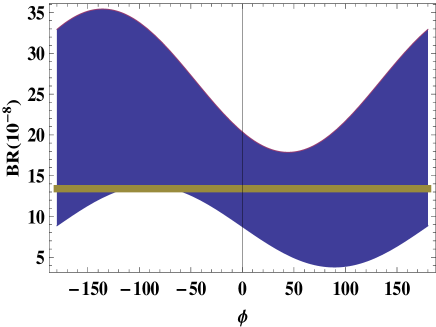
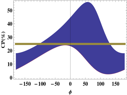
Figure 1: After setting $\xi=0.01$, the variation of the CP averaged branching ratio (left panel) and direct CP asymmetry (in %) (right panel) as a function of the new weak phase $\phi$. We varied the unitary angle $\gamma\in(50^{\circ},110^{\circ})$. The horizontal lines are predicted in the SM.

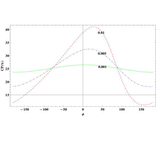
Figure 2: When setting $\gamma=70^{\circ}$, the variation of direct CP asymmetry with the new weak phase $\phi$, where the solid, dot-dashed and dashed lines correspond to $\xi=0.001,0.005$ and $0.01$.

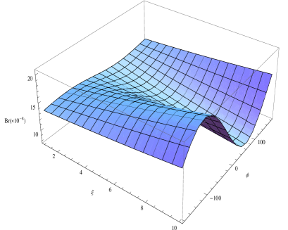
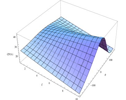
Figure 3: The variation of the CP averaged branching ratio (left panel) and the direct CP violation (right panel) with $\xi$ (in units of $10^{-3}$) and the new weak phase $\phi$.

Once obtaining the values of the Wilson coefficients at the scale $m_{b}$ and $\sqrt{\Lambda_{h}m_{b}}$, we can get the decay amplitude from the $Z^{\prime}$, analogous to Eq. (5), as:

$$\Delta{\cal A}(\overline{B_{s}^{0}}(p_{B})\to\phi(\epsilon,p_{1})\pi^{0}(p_{2}))=-i\frac{G_{F}}{2}2m_{\phi}f_{\pi}(\epsilon^{*}\cdot p_{B})A_{0}^{B_{s}\to\phi}(0)\\ \times\Big{[}V_{ub}V_{us}^{*}(\Delta a_{2}[u]+\Delta a_{3}[u]-\Delta a_{3}[d]-\Delta a_{5}[u]+\Delta a_{5}[d]-\Delta a_{7}[u]-\frac{1}{2}\Delta a_{7}[d]+\Delta a_{9}[u]+\frac{1}{2}\Delta a_{9}[d])\\ +V_{cb}V_{cs}^{*}(\Delta a_{3}[u]-\Delta a_{3}[d]-a_{5}[u]+\Delta a_{5}[d]-\Delta a_{7}[u]-\frac{1}{2}\Delta a_{7}[d]+\Delta a_{9}[u]+\frac{1}{2}\Delta a_{9}[d])\Big{]}.$$ (18)

To study the effect of the $Z^{\prime}$ boson, by setting $\xi=0.01$ and varying $\gamma$ within $50^{\circ}$ to $110^{\circ}$, one can get the variation of the CP averaged branching ratio and the direct CP asymmetry as a function of the new weak phase $\phi$, as shown in Fig. 1, where the horizontal lines are the values predicted in the SM. From these figures, we find that the branching ratio may become three times of that predicted in the SM or drop to one third of the SM value within the allowed parameter space. Moreover, as we mentioned before, we have introduced one new weak phase $\phi$ from the off-diagonal element of $B_{sb}^{L}$, which plays a major role in changing the direct CP asymmetry. The direct CP violation can reach $55\%$ if $\gamma=50^{\circ}$ and $\phi=70^{\circ}$. This remarkable enhancement will be an important signal in testing the model. Taking $\gamma=70^{\circ}$, we plot the variation of direct CP asymmetry as a function of the new weak phase $\phi$ with different $\xi=0.001,0.005,0.01$, as shown in Fig. 2. According to this figure, we note that the new physics effect cannot be detected if $\xi\leq 0.001$, namely a heavier $Z^{\prime}$ boson. If there exists a light $Z^{\prime}$ boson, the observation of this mode will in turn help us constraint the mass of $Z^{\prime}$. In Fig. 3, when leaving the $\xi$ and $\phi$ as free parameters, and setting $\gamma=70^{\circ}$, we present the correlations between the averaged branching ratio, direct CP asymmetry and the parameter values by the three-dimensional scatter plots. As illustrated in Fig. 3, the enhancement of both branching ratio and CP asymmetry cannot be fulfilled at the same parameter values.

To conclude, we have calculated the branching ratio and direct CP asymmetry of the decay mode $B_{s}\to\phi\pi^{0}$ within the QCD factorization approach in both the SM and the non-universal $Z^{\prime}$ model. This approach is suitable as the decay mode has no pollution from annihilation diagrams. Upon calculation, we found the branching ratio may be enlarged three times or decreased to one third by the effect of $Z^{\prime}$ boson within the allowed parameter space. Furthermore, as the direct CP asymmetry is concerned, it can reach $55\%$ with a light $Z^{\prime}$ boson and suitable CKM phase. Also, we note the enhancement of both branching ratio and CP asymmetry cannot be accomplished at the same parameter space. Thus, if this mode could be measured in the upcoming LHC-b experiment and/or Super B-factories it will provide a signal of the non-universal $Z^{\prime}$ model, and can be used to constrain the mass of the $Z^{\prime}$ boson in turn.

References

[1]
P. Langacker and M. Plumacher,
Phys. Rev. D 62, 013006 (2000)
[arXiv:hep-ph/0001204].
[2]
G. Buchalla, G. Burdman, C. T. Hill and D. Kominis,
Phys. Rev. D 53, 5185 (1996)
[arXiv:hep-ph/9510376].
[3]
E. Nardi,
Phys. Rev. D 48, 1240 (1993)
[arXiv:hep-ph/9209223].
[4]
V. Barger, et. al,
Phys. Lett. B 580, 186 (2004)
[arXiv:hep-ph/0310073];
V. Barger, et. al,
Phys. Lett. B 598, 218 (2004)
[arXiv:hep-ph/0406126];
V. Barger, et. al,
arXiv:0906.3745 [hep-ph];
V. Barger, et. al,
Phys. Rev. D 80, 055008 (2009)
[arXiv:0902.4507 [hep-ph]].
[5]
K. Cheung, et. al,
Phys. Lett. B 652, 285 (2007)
[arXiv:hep-ph/0604223];
C. W. Chiang, et. al,
JHEP 0608, 075 (2006)
[arXiv:hep-ph/0606122];
C. H. Chen and H. Hatanaka,
Phys. Rev. D 73, 075003 (2006)
[arXiv:hep-ph/0602140];
Q. Chang, X. Q. Li and Y. D. Yang,
JHEP 0905, 056 (2009)
[arXiv:0903.0275 [hep-ph]];
Q. Chang, X. Q. Li and Y. D. Yang,
arXiv:0907.4408 [hep-ph],
C. H. Chen,
arXiv:0911.3479 [hep-ph];
C. W. Chiang, R. H. Li and C. D. Lu,
arXiv:0911.2399 [hep-ph];
R. Mohanta and A. K. Giri,
Phys. Rev. D 79, 057902 (2009)
[arXiv:0812.1842 [hep-ph]].
[6]
P. Langacker,
arXiv:0801.1345 [hep-ph].
[7]
M. Beneke, G. Buchalla, M. Neubert and C. T. Sachrajda,
Phys. Rev. Lett. 83, 1914 (1999)
[arXiv:hep-ph/9905312];
M. Beneke, G. Buchalla, M. Neubert and C. T. Sachrajda,
Nucl. Phys. B 591, 313 (2000)
[arXiv:hep-ph/0006124].
[8]
M. Beneke and M. Neubert,
Nucl. Phys. B 675, 333 (2003)
[arXiv:hep-ph/0308039].
[9]
A. Ali, et.al,
Phys. Rev. D 76, 074018 (2007)
[arXiv:hep-ph/0703162].
[10] For a review, see G. Buchalla, A.J. Buras,
M.E. Lautenbacher, Rev. Mod. Phys. 68, 1125 (1996).
[11]
S. Chaudhuri, S. W. Chung, G. Hockney and J. Lykken,
Nucl. Phys. B 456, 89 (1995);
G. Cleaver, M. Cvetic, J. R. Espinosa, L. L. Everett, P. Langacker and
J. Wang,
Phys. Rev. D 59, 055005 (1999);
M. Cvetic, G. Shiu and A. M. Uranga,
Phys. Rev. Lett. 87, 201801 (2001);
M. Cvetic, P. Langacker and G. Shiu,
Phys. Rev. D 66, 066004 (2002).
[12]
T.K. Kuo, N. Nkagawam, Phys. Rev. D 66, 066004 (1984);
V.D. Barger, et.al, Int. J. Mod. A 2, 1327 (1987).
[13]
A.J. Buras, R. Fleischer, S. Recksiegel and F. Schwab, Phys. Rev.
Lett. 92, 101804 (2004)